The Magnetic Field and Impedances in Three-Phase Rectangular Busbars with a Finite Length

Abstract

The paper presents an analytical method for calculating impedances of rectangular bus ducts. The method is based on the partial inductance theory—in particular, the impedance of rectangular busbars in a three-phase system with a neutral conductor is described. The results of resistances and reactances of these systems of multiple rectangular conductors were obtained. Skin and proximity effects were taken into account. The measurements of the impedance of shielded and unshielded high-current busducts of rectangular conductors were also carried out. The magnetic field of the busbars was determined with several methods.

1. Introduction

Electrical connections between the main devices and the apparatus of power substations, which conduct a current of considerable value, are usually made of bare aluminum or copper conductors fixed on post insulators which are called busbars or bars [1,2]. Rigid busbars for each phase are usually made of individual flat bars. Only at higher currents do they consist of two or three flat bars in a package [3].

High-current bus ducts with copper or aluminum rectangular busbars are often used in switching stations and power substations due to their ease of assembly and operation. Their rated currents reach values of up to 10 kA and rated voltages are usually 10–30 kV [4]. A typical high-current bus duct with rectangular busbars is shown in Figure 1.

Due to electromagnetic coupling, currents in phase busbars induce eddy currents in the metal conductive shield. Hence, there is a complex electromagnetic coupling between phase busbars and the enclosure of the bus duct system. In the case of a parallel conductor system, the uneven distribution of current density in these conductors is caused by the skin effect as well as the proximity effect [6,7,8,9,10,11], which affect their self and mutual impedances [12,13,14,15,16,17]. Both the skin effect and proximity effect will generally cause the resistance of the busbars to increase and the inductance to decrease [18]. Defining these impedances is the purpose of this paper.

For every busbar, it is necessary to check the magnetic field in its surroundings to make sure it does not exceed the limit values set by the relevant standard [19,20,21,22]. This requires measurements around bus bar systems. Measurements of magnetic fields in such systems can be troublesome due to inaccessible places under the shield.

2. Impedances Rectangular Busbars with a Finite Length

The test objects of the bus duct, manufactured by the Holduct company (Myslowice, Poland), were two bus duct versions—the unshielded version shown in Figure 2 and the shielded version shown in Figure 3.

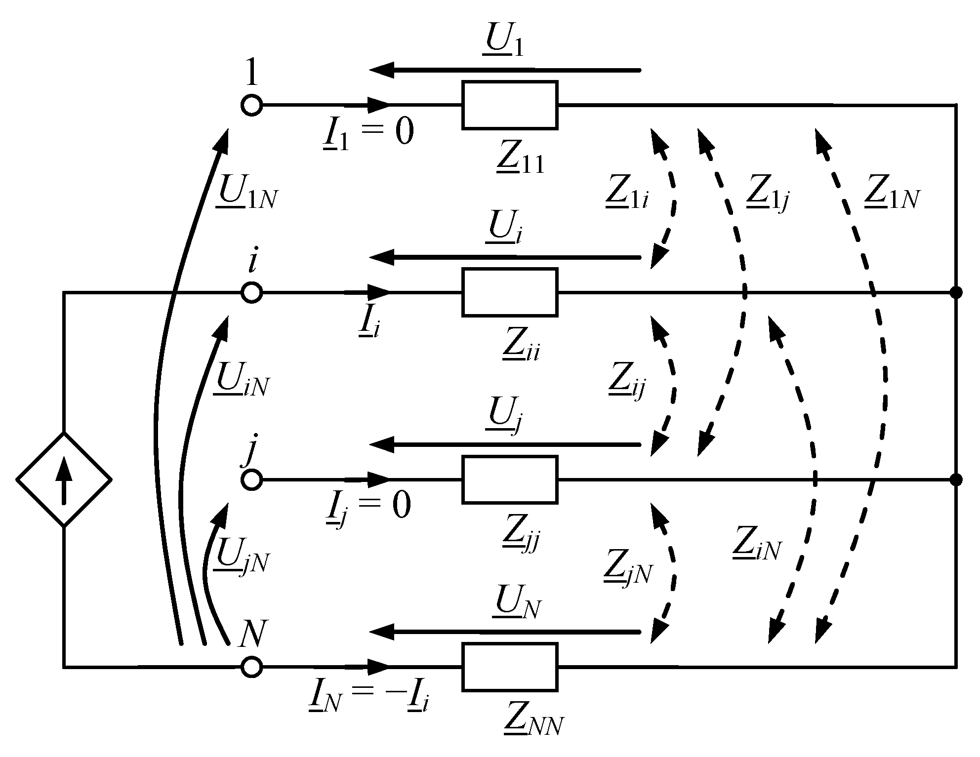
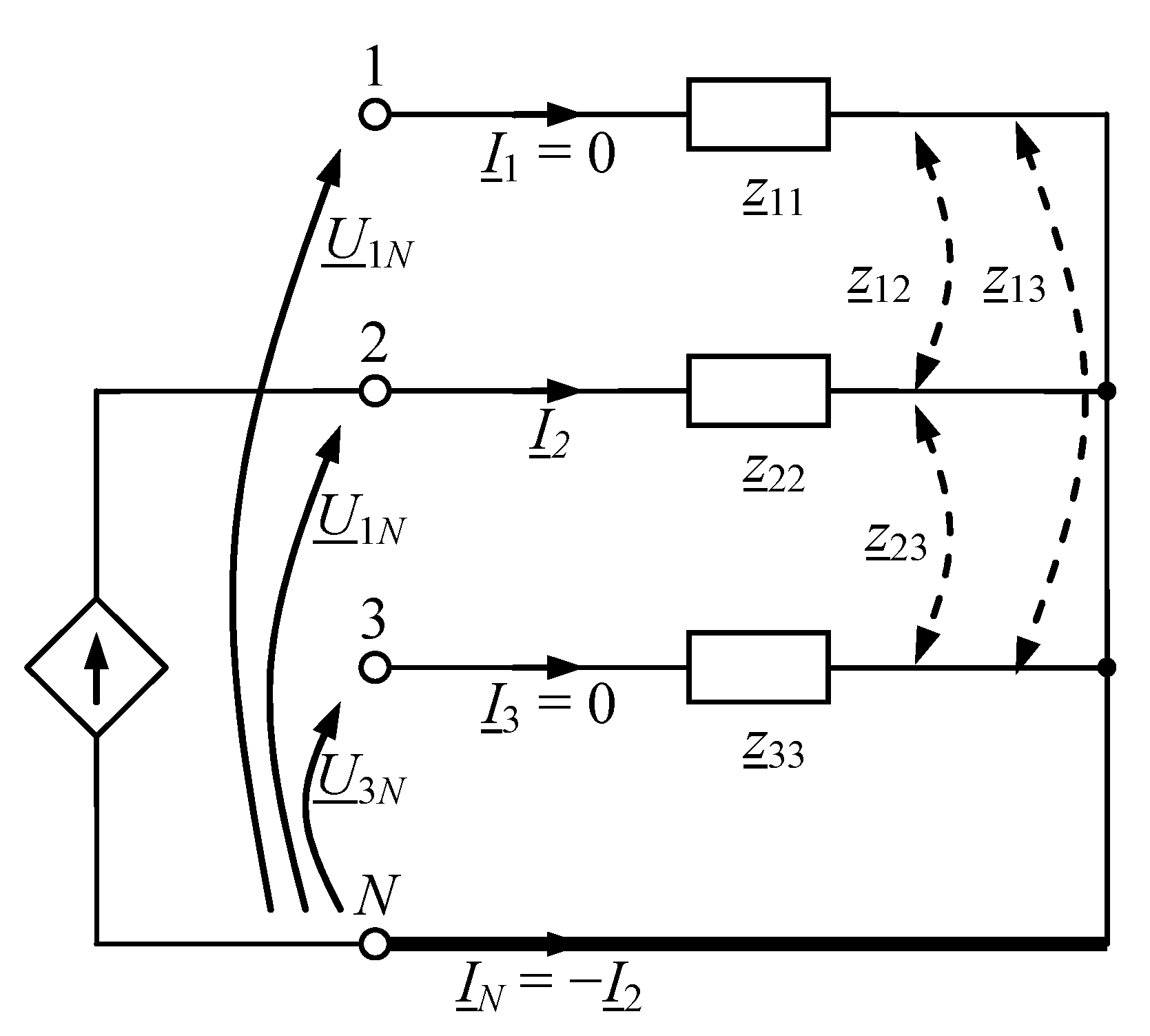
2.1. Impedance—Analytic Equations

In the case of N parallel conductors with length land conductivity σ_i (i = 1, 2,…, N) and a cross-section S_i with sinusoidal currents with angular frequency ω and complex effective values I_i directed in accordance with the Oz axis, the complex current density has only one component along this axis, that is

$${\underset{\_}{\mathit{J}}}_{\mathit{i}}(X)={\mathbf{1}}_z{\underset{\_}{J}}_i(X)$$

(1)

where X = X(x₁, y₁, z₁) is the point of observation, and 1_z is a z-axis versor.

If Ohms law is

$${\underset{\_}{\mathit{J}}}_i(X)={\sigma }_i{\underset{\_}{\mathit{E}}}_i(X)$$

(2)

and the voltage drop u_i per busbar unit length is added, the following integral equation is obtained for the l-th wire [18,23]

$$\frac{{\underset{\_}{J}}_i(X)}{{\sigma }_i}+\frac{\mathrm{j}\omega {\mathsf{\mu }}_0}{4\mathsf{\pi }}{\displaystyle \sum _{j=1}^N{\displaystyle \underset{v_j}{\int }\frac{{\underset{\_}{J}}_j(Y)}{{\rho }_{XY}}}\mathrm{d}{v}_j}={\underset{\_}{u}}_i$$

(3)

or

$$\frac{{\underset{\_}{J}}_i(X)}{{\sigma }_i}+\frac{\mathrm{j}\omega {\mathsf{\mu }}_0}{4\mathsf{\pi }}{\displaystyle \underset{v_i}{\int }\frac{{\underset{\_}{J}}_i(Y)}{{\rho }_{XY}}}\mathrm{d}{v}_i+\frac{\mathrm{j}\omega {\mathsf{\mu }}_0}{4\mathsf{\pi }}{\displaystyle \sum _{\begin{array}{l}j=1\\ j\ne i\end{array}}^N{\displaystyle \underset{v_j}{\int }\frac{{\underset{\_}{J}}_j(Y)}{{\rho }_{XY}}}\mathrm{d}{v}_j}={\underset{\_}{u}}_i$$

(4)

where Y = Y(x₂, y₂, z₂) is the source point, ${\rho }_{XY}=\sqrt{{\left(x_2-x_1\right)}^2+{\left(y_2-y_1\right)}^2+{\left(z_2-z_1\right)}^2}$ is the distance between the observation point X and the source point, v_i and v_j are the volumes of the i-th and j-th conductor respectively, and u_i is the unit voltage drop (in V∙m⁻¹) along the i-th conductor, where i, j = 1, 2,…, N. Unit voltage drop has a physical meaning only if all conductors of the circuit have been considered. However from the mathematical point of view, sometimes it is useful to split the circuit into several segments, e.g., particular busbars.

In the case presented in Figure 3, the integral equation for each busbar and enclosure is recorded in the form

$$\frac{{\underset{\_}{J}}_{i,k}(X)}{{\sigma }_i}+\frac{\mathrm{j}\omega {\mathsf{\mu }}_0}{4\mathsf{\pi }}{\displaystyle \sum _{j=1}^{N_c}{\displaystyle \sum _{l=1}^{N_j}{\displaystyle \underset{v_{j,l}}{\int }\frac{{\underset{\_}{J}}_{j,l}(Y)}{{\rho }_{XY}}}\mathrm{d}{v}_{j,l}}}={\underset{\_}{u}}_i$$

(5)

where N_c is the number of phases plus the neutral circuit plus the shield; i, j = 1, 2,…, N_c (N_c = 5); N_j is the number of busbars per phase or neutral circuit or the number of enclosure plates (usually 4); k, l = 1, 2,…, N_j.

If the current density functions J_i,k(X) and J_j,l(Y) are unknown or difficult to determine, then each of the conductors of the system shown in Figure 3, including the conductive plates of the enclosure, can be divided into elementary conductors [18,23].

Division of the k-th rectangular busbar with an i-th phase or neutral circuit is made separately in the horizontal (Ox axis) and vertical (Oy axis) directions. In this way, rectangular elementary conductors are obtained along with widths Δa and heights Δb respectively, determined by the following formulas:

$$\Delta a=\frac{a}{N_x^{(i,k)}}\mathrm{and}\Delta b=\frac{b}{N_y^{(i,k)}}$$

(6)

where a and b are, respectively, the width and height of a rectangular busbar, and N_x^(i,k) and N_y^(i,k) are, respectively, the numbers of divisions along the busbar width and height. Therefore, the total number of elementary conductors of the k-th busbar within an i-th phase is N_i,k = N_x^(i,k)⋅N_y^(i,k) and are numbered by m = 1, 2,…, N_i,k. For the l-th busbar with an j-th phase or the neutral circuit, the total number of elementary conductors is N_j,l = N_x^(j,l)⋅N_y^(j,l) and are numbered by n = 1, 2,…, N_j,l. The horizontal enclosure plate is divided N_x^(5,k) in the horizontal direction and N_ty^(5,k) in the vertical direction. The vertical plate of the enclosure is divided into N_tx^(5,k) and N_y^(5,k) segments along the horizontal and vertical directions, respectively, i.e.,

$$\Delta A=\frac{A}{N_x^{(5,k)}},\Delta B=\frac{B}{N_y^{(5,k)}},\Delta t_y=\frac{t}{N_{ty}^{(5,k)}}\mathrm{and}\Delta t_x=\frac{t}{N_{tx}^{(5,k)}}$$

(7)

where A and B are the widths of two horizontal and two vertical cover plates, respectively, t is their thickness, and k = 1, 2. All elementary conductors have the same length l.

If the cross-sectional area S_i,k^(m) = Δa · Δb of the m-th elemental conductor is very small [18], i.e., if the diagonal $\sqrt{{\left(\mathsf{\Delta }a\right)}^2+{\left(\mathsf{\Delta }b\right)}^2}$ of this cross-section is not greater than the depth of penetration of the electromagnetic wave, then in such an elementary conductor the skin effect can be neglected and then the constant complex current density in the whole cross-section can be assumed in the form of

$${\underset{\_}{J}}_{i,k}^{(m)}=\frac{{\underset{\_}{I}}_{i,k}^{(m)}}{S_{i,k}^{(m)}}$$

(8)

where I_i,k^(m) is a complex current in the m-th elementary conductor.

Then also for the m-th elementary conductor, an equation can be written

$$\frac{{\underset{\_}{J}}_{i,k}^{(m)}(X)}{{\sigma }_i}+\frac{\mathrm{j}\omega {\mathsf{\mu }}_0}{4\mathsf{\pi }}{\displaystyle \sum _{j=1}^{N_c}{\displaystyle \sum _{l=1}^{N_j}{\displaystyle \sum _{n=1}^{N_{j,l}}{\displaystyle \underset{v_{j,l}}{\int }\frac{{\underset{\_}{J}}_{j,l}^{(n)}(Y)}{{\rho }_{XY}}}\mathrm{d}{v}_{j,l}^{(n)}}}}={\underset{\_}{u}}_i$$

(9)

where v_j,l⁽ⁿ⁾ is the volume of the n-th elementary conductor of the busbar or the shield of the l-th busbar with the j-th phase of the neutral circuit or the enclosure.

Then Equation (9) is divided by the area S_i,k^(m) and integrated throughout volume v_i,k^(m) of the m-th elementary conductor, giving the equation

$$R_{i,k}^{(m)}{\underset{\_}{I}}_{i,k}^{(m)}+\mathrm{j}\omega {\displaystyle \sum _{j=1}^{N_c}{\displaystyle \sum _{l=1}^{N_j}{\displaystyle \sum _{n=1}^{N_{j,l}}{M}_{(i,k)(j,l)}^{(m,n)}{\underset{\_}{I}}_{j,l}^{(n)}}}}={\underset{\_}{U}}_i$$

(10)

where U_i is the voltage drop in the elementary conductor of the i-th phase of the neutral conductor or the enclosure.

In the above equation, the resistance of the m-th elementary conductor is

$$R_{i,k}^{(m)}=\frac{l}{{\sigma }_i{S}_{i,k}^{(m)}}$$

(11)

and its self inductance or mutual inductance between two elementary conductors is

$$M_{(i,k)(j,l)}^{(m,n)}=\frac{{\mathsf{\mu }}_0}{4\mathsf{\pi }{S}_{i,k}^{(m)}{S}_{j,l}^{(n)}}{\displaystyle \underset{v_{i,k}^{(m)}}{\int }{\displaystyle \underset{v_{j,l}^{(n)}}{\int }\frac{\mathrm{d}{v}_{i,k}^{(m)}\mathrm{d}{v}_{j,l}^{(n)}}{{\rho }_{XY}}}}$$

(12)

The integrals can be performed analytically, the final closed forms for the inductance given in [24,25,26,27].

The equation system of (10) written for each elementary conductor is a complex linear equation system

$$\underset{\_}{\widehat{\mathit{U}}}=\underset{\_}{\widehat{\mathit{Z}}}\underset{\_}{\widehat{\mathit{I}}}$$

(13)

where $\underset{\_}{\widehat{\mathit{U}}}$ and $\underset{\_}{\widehat{\mathit{I}}}$ are, respectively, columnar voltage and current vectors in each of the elementary conductors, and $\underset{\_}{\widehat{\mathit{Z}}}$ is the symmetrical matrix of self and mutual impedances—the so-called impedance matrix of all elementary conductors.

The current $\underset{\_}{\widehat{\mathit{I}}}$ and voltage $\underset{\_}{\widehat{\mathit{U}}}$ vectors can be represented as follows:

$$\underset{\_}{\widehat{\mathit{U}}}=\left\{\begin{array}{c}{\left\{\underset{\_}{U}\right\}}_1\\ {\left\{\underset{\_}{U}\right\}}_2\\ ⋮\\ {\left\{\underset{\_}{U}\right\}}_{N_c}\end{array}\right\},\hspace{1em} {\left\{\underset{\_}{U}\right\}}_i=\left\{\begin{array}{c}{\left\{\underset{\_}{U}\right\}}_{i,1}\\ ⋮\\ {\left\{\underset{\_}{U}\right\}}_{i,N_i}\end{array}\right\},\hspace{1em} {\left\{\underset{\_}{U}\right\}}_{i,k}=\left\{{\underset{\_}{U}}_i\right\}\mathrm{of}\mathrm{length}{N}^{(i,k)}$$

(14)

and

$$\underset{\_}{\widehat{\mathit{I}}}=\left\{\begin{array}{c}{\left\{\underset{\_}{I}\right\}}_1\\ {\left\{\underset{\_}{I}\right\}}_2\\ ⋮\\ {\left\{\underset{\_}{I}\right\}}_{N_c}\end{array}\right\},\hspace{1em} {\left\{\underset{\_}{I}\right\}}_i=\left\{\begin{array}{c}{\left\{\underset{\_}{I}\right\}}_{i,1}\\ ⋮\\ {\left\{\underset{\_}{I}\right\}}_{i,N_i}\end{array}\right\},\hspace{1em} {\left\{\underset{\_}{I}\right\}}_{i,k}=\left\{{\underset{\_}{I}}_{i,k}^{(n)}\right\}\mathrm{of}\mathrm{length}{N}^{(i,k)}$$

(15)

The impedance matrix $\underset{\_}{\widehat{\mathit{Z}}}$ is a matrix whose elements (sub-matrices) are also matrices

$$\underset{\_}{\widehat{\mathit{Z}}}=\left[\begin{array}{cccc}[{\underset{\_}{Z}}_{(1,k)(1,l)}^{(m,n)}]& [{\underset{\_}{Z}}_{(1,k)(2,l)}^{(m,n)}]& \cdots & [{\underset{\_}{Z}}_{(1,k)(N_c,l)}^{(m,n)}]\\ [{\underset{\_}{Z}}_{(2,k)(1,l)}^{(m,n)}]& [{\underset{\_}{Z}}_{(2,k)(2,l)}^{(m,n)}]& \cdots & [{\underset{\_}{Z}}_{(2,k)(N_c,l)}^{(m,n)}]\\ ⋮& ⋮& \ddots & ⋮\\ [{\underset{\_}{Z}}_{(N_c,k)(1,l)}^{(m,n)}]& [{\underset{\_}{Z}}_{(N_c,k)(2,l)}^{(m,n)}]& \cdots & [{\underset{\_}{Z}}_{(N_c,k)(N_c,l)}^{(m,n)}]\end{array}\right]$$

(16)

where sub-matrices $\left[Z_{\left(i,k\right)\left(j,l\right)}^{\left(m,n\right)}\right]$ have an elements containing self impedances and mutual impedances between the conductors of the i-th and the j-th phase:

$$\left[{\underset{\_}{Z}}_{(i,k)(j,l)}^{(m,n)}\right]=\left[\begin{array}{ccc}[{\underset{\_}{Z}}_{(j,1)(i,1)}^{(m,n)}]& \dots & [{\underset{\_}{Z}}_{(j,1)(i,N_i)}^{(m,n)}]\\ ⋮& \ddots & ⋮\\ [{\underset{\_}{Z}}_{(j,N_j)(i,1)}^{(m,n)}]& \dots & [{\underset{\_}{Z}}_{(j,N_j)(i,N_i)}^{(m,n)}]\end{array}\right]$$

(17)

The elements of the matrix $\underset{\_}{\widehat{\mathit{Z}}}$ are

$${\underset{\_}{Z}}_{(i,k)(j,l)}^{(m,n)}=\{\begin{array}{ll}{R}_{i,k}^{(m)}+\mathrm{j}\omega M_{(i,k)(j,l)}^{(m,n)}\hfill & \mathrm{for}m=n,i=j,k=l\hfill \\ \mathrm{j}\omega M_{(i,k)(j,l)}^{(m,n)}\hfill & \mathrm{otherwise}.\hfill \end{array}$$

(18)

The admittance matrix $\underset{\_}{\widehat{\mathit{Y}}}$ is then found, which is the inverse impedance matrix and is given by the formula

$$\underset{\_}{\widehat{\mathit{Y}}}={\left[{\underset{\_}{Y}}_{(i,k)(j,l)}^{(m,n)}\right]}^{}={\underset{\_}{\widehat{\mathit{Z}}}}^{-1}$$

(19)

It is then possible to determine the current in the m-th elementary conductor of the k-th conductor of the i-th phase or the neutral circuit as

$${\underset{\_}{I}}_{i,k}^{(m)}={\displaystyle \sum _{j=1}^{N_c}{\displaystyle \sum _{l=1}^{N_j}{\displaystyle \sum _{n=1}^{N_{j,l}}{\underset{\_}{Y}}_{(i,k)(j,l)}^{(m,n)}{\underset{\_}{U}}_j}}}$$

(20)

Therefore, the total current of the i-th phase or the neutral circuit is expressed by the sum

$${\underset{\_}{I}}_i={\displaystyle \sum _{k=1}^{N_i}{\displaystyle \sum _{m=1}^{N_{i,k}}{\underset{\_}{I}}_{i,k}^{(m)}}}$$

(21)

After substitution of (20) to (21), the following is obtained:

$${\underset{\_}{I}}_i={\displaystyle \sum _{j=1}^{N_c}{\underset{\_}{Y}}_{i,j}{\underset{\_}{U}}_j}$$

(22)

where

$${\underset{\_}{Y}}_{i,j}={\displaystyle \sum _{k=1}^{N_i}{\displaystyle \sum _{m=1}^{N_{i,k}}{\displaystyle \sum _{l=1}^{N_j}{\displaystyle \sum _{n=1}^{N_{j,l}}{\underset{\_}{Y}}_{(i,k)(j,l)}^{(m,n)}}}}}$$

(23)

The admittance matrix, with elements given by (23), will allow the determination of the impedance matrix of the shielded three-phase high-current bus duct with a neutral conductor with rectangular busbars on the basis of the formula

$$\underset{\_}{\mathit{Z}}=\left[{\underset{\_}{Z}}_{i,j}\right]={\underset{\_}{\mathit{Y}}}^{-1}={\left[{\underset{\_}{Y}}_{i,j}\right]}^{-1}$$

(24)

Because impedances Z_i,j are determined from the matrix, which is determined only from the design of the high-current busduct and material properties, its value does not depend on the phase currents and the current in the neutral circuit. Skin and proximity effects are taken into account.

The impedances of the high-current busduct shown in Figure 3 are given by a $4\times 4$ matrix. In circuit theory, impedances Z_ii and Z_ij are called partial self and mutual impedances which, however, should not be misinterpreted as the classical definition of self and mutual impedances in closed circuits [28].

Impedances Z_ii and Z_j are sufficient to describe the behavior of the electric circuit but do not have a physical interpretation and therefore cannot be determined by measurement. If however, one of the busbars, e.g., the N-th, were to be regarded as a so-called reference conductor, it could be used as a return conductor for other conductors. If, for example, only phase current I_i exists, its return to the power source is via the neutral bus (Figure 4). This means that this current forms a closed loop i-N. Thereafter, complex voltages, such as voltage drops and the voltage induced by the current I_i, are described by the following classic formulas [18]:

$${\underset{\_}{U}}_i={\underset{\_}{Z}}_{ii}{\underset{\_}{I}}_i+{\underset{\_}{Z}}_{iN}{\underset{\_}{I}}_N=({\underset{\_}{Z}}_{ii}-{\underset{\_}{Z}}_{iN}){\underset{\_}{I}}_i$$

(25)

$${\underset{\_}{U}}_j={\underset{\_}{Z}}_{ji}{\underset{\_}{I}}_i+{\underset{\_}{Z}}_{jN}{\underset{\_}{I}}_N=({\underset{\_}{Z}}_{ji}-{\underset{\_}{Z}}_{jN}){\underset{\_}{I}}_i$$

(26)

$${\underset{\_}{U}}_N={\underset{\_}{Z}}_{Ni}{\underset{\_}{I}}_i+{\underset{\_}{Z}}_{NN}{\underset{\_}{I}}_N=({\underset{\_}{Z}}_{Ni}-{\underset{\_}{Z}}_{NN}){\underset{\_}{I}}_i$$

(27)

The voltage between the terminals i-N is described by the equation

$${\underset{\_}{U}}_{iN}={\underset{\_}{U}}_i-{\underset{\_}{U}}_N=({\underset{\_}{Z}}_{ii}-{\underset{\_}{Z}}_{iN}-{\underset{\_}{Z}}_{Ni}+{\underset{\_}{Z}}_{NN}){\underset{\_}{I}}_i$$

(28)

and the voltage between the terminals j-N has the form of

$${\underset{\_}{U}}_{jN}={\underset{\_}{U}}_j-{\underset{\_}{U}}_N=({\underset{\_}{Z}}_{ji}-{\underset{\_}{Z}}_{jN}-{\underset{\_}{Z}}_{Ni}+{\underset{\_}{Z}}_{NN}){\underset{\_}{I}}_i$$

(29)

After that, the definition of the self impedance of the loop i-N is introduced as

$${\underset{\_}{z}}_{ii}=\frac{{\underset{\_}{U}}_{iN}}{{\underset{\_}{I}}_i}={\underset{\_}{Z}}_{ii}-{\underset{\_}{Z}}_{iN}-{\underset{\_}{Z}}_{Ni}+{\underset{\_}{Z}}_{NN}={\underset{\_}{Z}}_{ii}+{\underset{\_}{Z}}_{NN}$$

(30)

and the mutual impedance definition between the loop i-N and j-N as

$${\underset{\_}{z}}_{ji}=\frac{{\underset{\_}{U}}_{jN}}{{\underset{\_}{I}}_i}={\underset{\_}{Z}}_{ji}-{\underset{\_}{Z}}_{jN}-{\underset{\_}{Z}}_{Ni}+{\underset{\_}{Z}}_{NN}$$

(31)

As a result, the square impedance matrix $\left(n-1\right)\times \left(n-1\right)$ is obtained with the elements z_ii and z_ji. This matrix is called a reduced impedance matrix which, in the case of Figure 3, has the form of

$$\underset{\_}{\mathit{z}}=\left[\begin{array}{ccc}{\underset{\_}{z}}_{11}& {\underset{\_}{z}}_{12}& {\underset{\_}{z}}_{13}\\ {\underset{\_}{z}}_{21}& {\underset{\_}{z}}_{22}& {\underset{\_}{z}}_{23}\\ {\underset{\_}{z}}_{31}& {\underset{\_}{z}}_{32}& {\underset{\_}{z}}_{33}\end{array}\right]$$

(32)

Afterwards, the electric circuit model of the three-phase high-current busduct with the neutral busbar contains only three self impedances and six mutual impedances (Figure 5).

If the shield of the high-current bus duct is grounded at its ends by resistance R_gr (Figure 6), then the unknown current of the shield grounding equals

$${\underset{\_}{I}}_5={\underset{\_}{I}}_{en}={\displaystyle \sum _{j=1}^4{\underset{\_}{Y}}_{5,j}{\underset{\_}{U}}_j+}{\underset{\_}{Y}}_{5,5}{\underset{\_}{U}}_{en}$$

(33)

In addition, pursuant to Kirchhoff’s second law (Figure 6):

$${\underset{\_}{U}}_{en}+2R_{gr}{\underset{\_}{I}}_{en}=0$$

(34)

By solving Equations (33) and (34) given the ${\underset{\_}{U}}_{en}$ we obtain

$${\underset{\_}{U}}_{en}={\underset{\_}{U}}_5=\frac{-1}{{\underset{\_}{Y}}_{5,5}+\frac{1}{2R_{gr}}}\left[{\displaystyle \sum _{j=1}^5{\underset{\_}{Y}}_{i,j}{\underset{\_}{U}}_j+{\underset{\_}{Y}}_{5,4}{\underset{\_}{U}}_0}\right]$$

(35)

Substituting solution (35) to the Equation (22) we obtain

$${\underset{\_}{I}}_i={\displaystyle \sum _{j=1}^4{\underset{\_}{\tilde{Y}}}_{i,j}\underset{\_}{Y}{\underset{\_}{U}}_j}$$

(36)

where ${\underset{\_}{I}}_4={\underset{\_}{I}}_0{\displaystyle \sum _{j=1}^4{\underset{\_}{\tilde{Y}}}_{i,j}\underset{\_}{Y}{\underset{\_}{U}}_j}$.

Next, the admittance

$${\underset{\_}{\tilde{Y}}}_{i,j}={\underset{\_}{Y}}_{i,j}-\frac{{\underset{\_}{Y}}_{i,5}{\underset{\_}{Y}}_{5,j}}{{\underset{\_}{Y}}_{5,5}+\frac{1}{2R_{uz}}}\mathrm{for}i,j=1,2,3,4$$

(37)

from which, after calculating the inverse matrix, an impedance matrix is obtained

$${\underset{\_}{\tilde{Z}}}_{i,j}={\left[{\underset{\_}{\tilde{Y}}}_{i,j}\right]}^{-1}$$

(38)

2.2. Impedances—Calculation Example

In order to verify the obtained formulas, impedance measurements were made on an actual high-current busduct (Figure 7).

The impedances of the busbars were determined by the following methods: the analytical method (AM) previously described [1,3,29] for simple configurations of unshielded busbars neglecting skin and proximity effects, the integral equation method (IEM) based on integral equations [1,18,30,31], the two-dimensional finite element method (FEM) using FEMM software [32,33] and the measurement (meas) in the test stands presented in Figure 7.

In the case of an unshielded (Figure 2) and shielded (Figure 3) busbar type, phase conductors and neutral conductors contain one rectangular bar hence N₁ = N₂ = N₃ = 1 and N₄ = 1. As shown in Figure 2, the dimensions are: a = 12 mm, b = 100 mm, and d = d₁ = 24 mm. The phase bars and the neutral bar are copper bars with a conductivity of σ = 56 MS∙m⁻¹. The frequency of the phase currents is f = 50 Hz.

For the calculations, it was assumed that l = 1 m and l = 3.50 m. The last length is also the length of the actual busbar tested in the laboratory. Each bar is divided into N_x^(i,k) = 12 and N_y^(i,k) = 50, which gives 600 rectangular elemental bars for each bar, i.e., the total number of elementary bars with dimensions of $2\times 1$ mm is 2400.

The busbar enclosure (Figure 3) is made of aluminum with a conductivity of σ₅ = 34 MS∙m⁻¹ and the thickness of its walls t = 3 mm. The position of the enclosure walls relative to the bars is determined by a₁ = 12 mm, b₁ = 12 mm, b₂ = 15 mm. The horizontal enclosure plate is divided into N_x^(5,k) = 114 and N_ty^(5,k) = 2, which gives 228 elementary rectangular conductors measuring $1\times 1.5$ mm. The vertical enclosure plate is divided into N_y^(5,k) = 127 and N_tx^(5,k) = 2, giving 254 elementary conductors of 1 × 1.5 mm. In this way, the enclosure is divided into 964 rectangular elementary conductors. Therefore, the total number of rectangular elementary conductors of the busbar from Figure 3 is 3364.

After the aforementioned discretization was performed, the self and mutual impedances of the unshielded and shielded busbar systems with one rectangular bar per phase and with one neutral bar were calculated. The results from the calculations are summarized in

Table 1. Self and mutual impedances in mΩ of the unshielded (u) and shielded (s) three-phase busbar systems illustrated in Figure 2 and Figure 3.

Length l in m		Ni		s	Method	1 (L1)	2 (L2)	3 (L3)	4 (N)
	Nj		u
1	1 (L1)		u		AM	0.014 + j 0.214	0.000 + j 0.185	0.000 + j 0.161	0.000 + j 0.185
					IEM	0.022 + j 0.202	0.005 + j 0.173	0.002 + j 0.149	0.004 + j 0.174
					FEM	0.021 + j 0.339	0.005 + j 0.339	0.002 + j 0.288	0.004 + j 0.312
			s		IEM	0.025 + j 0.199	0.006 + j 0.174	0.000 + j 0.153	0.008 + j 0.168
					FEM	0.023 + j 0.337	0.005 + j 0.312	–0.005 + j 0.292	0.008 + j 0.306
	2 (L2)		u		AM	0.000 + j 0.185	0.014 + j 0.214	0.000 + j 0.185	0.000 + j 0.161
					IEM	0.005 + j 0.173	0.019 + j 0.202	0.004 + j 0.174	0.002 + j 0.149
					FEM	0.005 + j 0.339	0.021 + j 0.339	0.004 + j 0.313	0.002 + j 0.288
			s		IEM	0.006 + j 0.174	0.025 + j 0.199	0.008 + j 0.168	0.000 + j 0.153
					FEM	0.008 + j 0.306	0.024 + j 0.337	0.008 + j 0.306	–0.005 + j 0.292
	3 (L3)		u		AM	0.000 + j 0.161	0.000 + j 0.185	0.014 + j 0.214	0.000 + j 0.143
					IEM	0.002 + j 0.149	0.004 + j 0.174	0.021 + j 0.203	0.000 + j 0.130
					FEM	0.002 + j 0.288	0.004 + j 0.174	0.021 + j 0.341	–0.001 + j 0.270
			s		IEM	0.000 + j 0.153	0.008 + j 0.168	0.031 + j 0.187	–0.007 + j 0.144
					FEM	–0.005 + j 0.292	0.008 + j 0.306	0.032 + j 0.324	–0.007 + j 0.283
	4 (N)		u		AM	0.000 + j 0.185	0.000 + j 0.161	0.000 + j 0.143	0.014 + j 0.214
					IEM	0.004 + j 0.174	0.002 + j 0.149	0.000 + j 0.130	0.021 + j 0.203
					FEM	0.004 + j 0.312	0.002 + j 0.288	–0.001 + j 0.270	0.021 + j 0.341
			s		IEM	0.008 + j 0.168	0.000 + j 0.153	–0.007 + j 0.144	0.031 + j 0.187
					FEM	0.008 + j 0.306	–0.005 + j 0.292	–0.007 + j 0.283	0.032 + j 0.324
3.50	1 (L1)		u		AM	0.053 + j 1.038	0.000 + j 0.935	0.000 + j 0.845	0.000 + j 0.935
					IEM	0.075 + j 0.990	0.016 + j 0.891	0.006 + j 0.808	0.015 + j 0.892
					FEM	0.049 + j 0.749	0.017 + j 1.186	0.007 + j 1.008	0.014 + j 1.092
			s		IEM	0.086 + j 0.983	0.020 + j 0.894	–0.002 + j 0.824	0.027 + j 0.876
					FEM	0.081 + j 1.179	0.017 + j 1.092	–0.017 + j 1.022	0.028 + j 1.071
	2 (L2)		u		AM	0.000 + j 0.935	0.053 + j 1.038	0.000 + j 0.935	0.000 + j 0.845
					IEM	0.016 + j 0.891	0.075 + j 0.990	0.015 + j 0.893	0.006 + j 0.808
					FEM	0.017 + j 1.186	0.074 + j 1.186	0.014 + j 1.095	0.007 + j 1.008
			s		IEM	0.020 + j 0.894	0.086 + j 0.982	0.028 + j 0.875	–0.002 + j 0.824
					FEM	0.017 + j 1.092	0.084 + j 1.179	0.028 + j 1.071	–0.017 + j 1.022
	3 (L3)		u		AM	0.000 + j 0.845	0.000 + j 0.935	0.053 + j 1.038	0.000 + j 0.778
					IEM	0.006 + j 0.823	0.015 + j 0.893	0.073 + j 0.995	0.000 + j 0.745
					FEM	0.007 + j 1.008	0.014 + j 1.095	0.073 + j 1.193	–0.003 + j 0.945
			s		IEM	–0.002 + j 0.824	0.028 + j 0.875	0.107 + j 0.940	–0.027 + j 0.792
					FEM	–0.017 + j 1.022	0.028 + j 1.071	0.112 + j 1.134	–0.024 + j 0.990
	4 (N)		u		AM	0.000 + j 0.935	0.000 + j 0.845	0.000 + j 0.778	0.053 + j 1.038
					IEM	0.015 + j 0.892	0.006 + j 0.808	0.000 + j 0.745	0.073 + j 1.012
					FEM	0.014 + j 1.092	0.007 + j 1.008	–0.003 + j 0.945	0.073 + j 0.994
			s		IEM	0.027 + j 0.876	–0.002 + j 0.824	–0.027 + j 0.792	0.105 + j 0.942
					FEM	0.028 + j 1.071	–0.017 + j 1.022	–0.024 + j 0.990	0.112 + j 1.134

u: unshielded; s: shielded.

.

The obtained results of the self and mutual impedance calculations presented in Table 1 allow determination of the reduced self and mutual impedances. These impedances are shown in

Table 2. Reduced self and mutual impedances in mΩ of the unshielded (u) and shielded (s) three-phase busbar systems illustrated in Figure 2 and Figure 3.

Length l in m		j		s	Methods	1 (L1)	2 (L2)	3 (L3)
	i		u
3.50	1 (L1)		u		AM	0.106 + j 0.206	0.053 + j 0.193	0.053 + j 0.170
					IEM	0.117 + j 0.199	0.068 + j 0.184	0.064 + j 0.165
					FEM	0.118 + j 0.198	0.068 + j 0.183	0.064 + j 0.163
					meas	0.113 + j 0.208	0.058 + j 0.192	0.053 + j 0.172
			s		IEM	0.137 + j 0.173	0.100 + j 0.136	0.103 + j 0.098
					FEM	0.138 + j 0.172	0.102 + j 0.133	0.108 + j 0.094
					meas	0.131 + j 0.178	0.089 + j 0.144	0.095 + j 0.106
	2 (L2)		u		AM	0.053 + j 0.193	0.106 + j 0.386	0.053 + j 0.350
					IEM	0.068 + j 0.184	0.136 + j 0.368	0.081 + j 0.333
					FEM	0.068 + j 0.183	0.136 + j 0.365	0.081 + j 0.330
					meas	0.058 + j 0.192	0.117 + j 0.384	0.075 + j 0.342
			s		IEM	0.100 + j 0.136	0.196 + j 0.276	0.163 + j 0.201
					FEM	0.102 + j 0.133	0.200 + j 0.270	0.170 + j 0.193
					meas	0.090 + j 0.145	0.177 + j 0.296	0.148 + j 0.218
	3 (L3)		u		AM	0.053 + j 0.170	0.053 + j 0.350	0.106 + j 0.520
					IEM	0.064 + j 0.165	0.081 + j 0.333	0.145 + j 0.498
					FEM	0.064 + j 0.163	0.081 + j 0.330	0.145 + j 0.493
					meas	0.052 + j 0.172	0.074 + j 0.342	0.128 + j 0.513
			s		IEM	0.103 + j 0.098	0.163 + j 0.201	0.267 + j 0.299
					FEM	0.108 + j 0.094	0.170 + j 0.193	0.279 + j 0.287
					meas	0.095 + j 0.105	0.145 + j 0.218	0.243 + j 0.329

u: unshielded; s: shielded.

. The table also presents the measurement results of these impedances. Impedance measurements were made on a suitably prepared measurement stand, as shown in Figure 7. The high-current bus duct was supplied with a current of 1 kA. The current measurement was carried out through Rogowski coils (AmpFLEX series A100) with an accuracy of 1%, and the voltage measurement was made using a digital voltmeter (Picotest M3500) with a class of 0.1%. The phase angle between current and voltage was measured using a phase meter (Dranetz Plug-in-Model-305-PA-3009A) with an accuracy of 1%. The experiments were performed under 50 Hz sinusoidal supply. The actual length of the bus duct was 3.9 m while in order to avoid the influence of the power cords, voltage drop measurements were made on a 3.5 m section. To calculate the reduced impedance matrix, effective values of current and voltage were measured as well as the phase angle between their instantaneous values. The measurements were repeated several times and the measured impedance values are presented in Table 2. The impedance values presented were compared to the results obtained using the integral equation method (IEM) (software was developed in the Visual Studio 2010 Professional environment), the finite elements method (FEM), and the measurement results (meas).

3. Magnetic Field of the Three-Phase Rectangular Busbars with a Finite Length

The magnetic field of busbars manufactured by the Holduct company were examined in unshielded bars (Figure 2) as well as shielded bars (Figure 3).

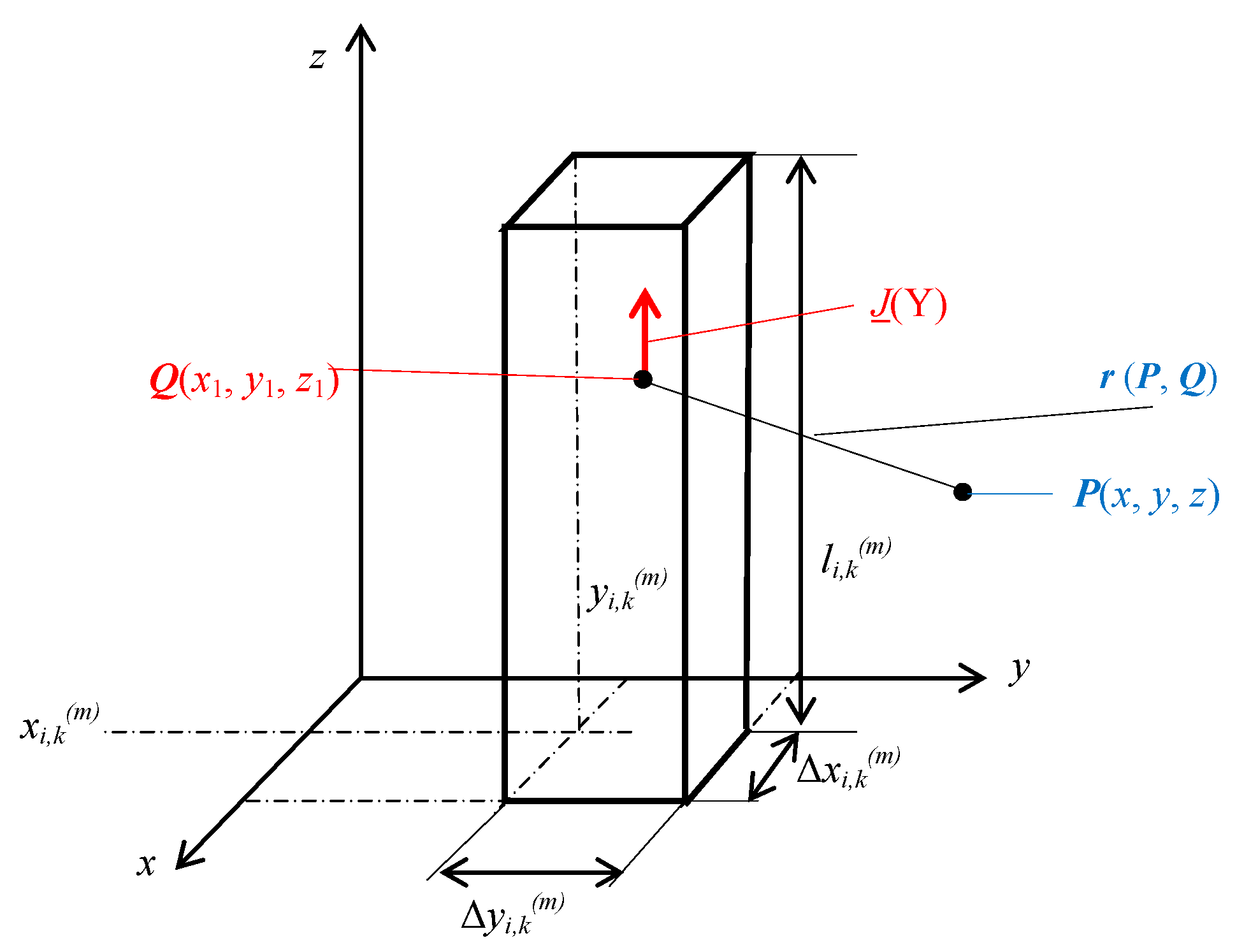
3.1. Current Densities at Rectangular Busducts

Knowledge of voltage drops on individual conductors U_j for j = 1, 2, 3, 4, 5 according to the substitution

$${\underset{\_}{U}}_{jl}^{(n)}={\underset{\_}{U}}_j$$

(39)

allows, by virtue of the formula [1]

$${\underset{\_}{I}}_{i,k}^{(m)}={\displaystyle \sum _{j=1}^5{\displaystyle \sum _{l=1}^{N_j}{\displaystyle \sum _{n=1}^{N_{j,l}}{\underset{\_}{Y}}_{(i,k)(j,l)}^{(m.n)}}}{\underset{\_}{U}}_{j,l}^{(n)}}$$

(40)

where $i=1,2,3,4,5;k=1,2,..,N_i;m=1,2,..,N_{i,k}$, to calculate the current at any m-th fiber of the k-th conductor of i-th phase

$${\underset{\_}{I}}_{i,k}^{(m)}={\displaystyle \sum _{j=1}^5\left({\displaystyle \sum _{l=1}^{N_j}{\displaystyle \sum _{n=1}^{N_{j,l}}{\underset{\_}{Y}}_{(i,k)(j,l)}^{(m.n)}}}{\underset{\_}{U}}_{j,l}^{(n)}\right)}$$

(41)

Once the currents in all elementary conductors are calculated, it allows, according to the formula

$${\underset{\_}{J}}_{i,k}^{(m)}=\frac{{\underset{\_}{I}}_{i,k}^{(m)}}{S_{i,k}^{(m)}}$$

(42)

to determine the current density distribution at the busducts and the screen.

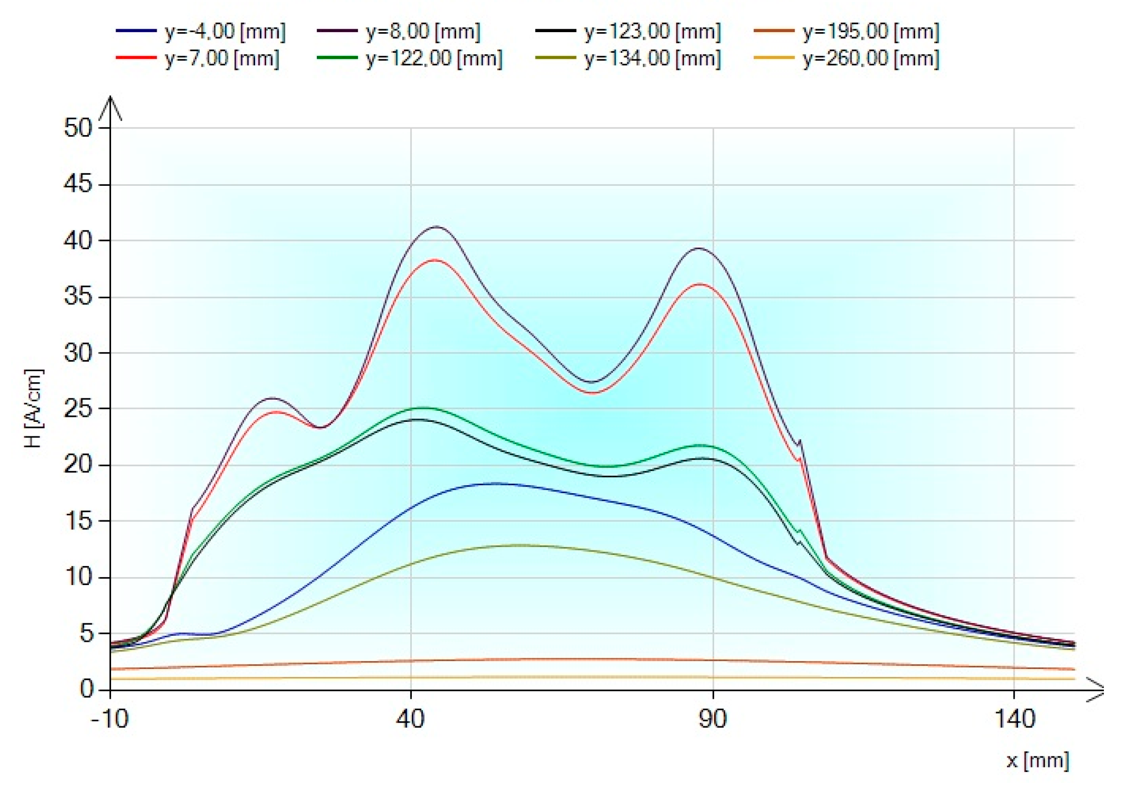
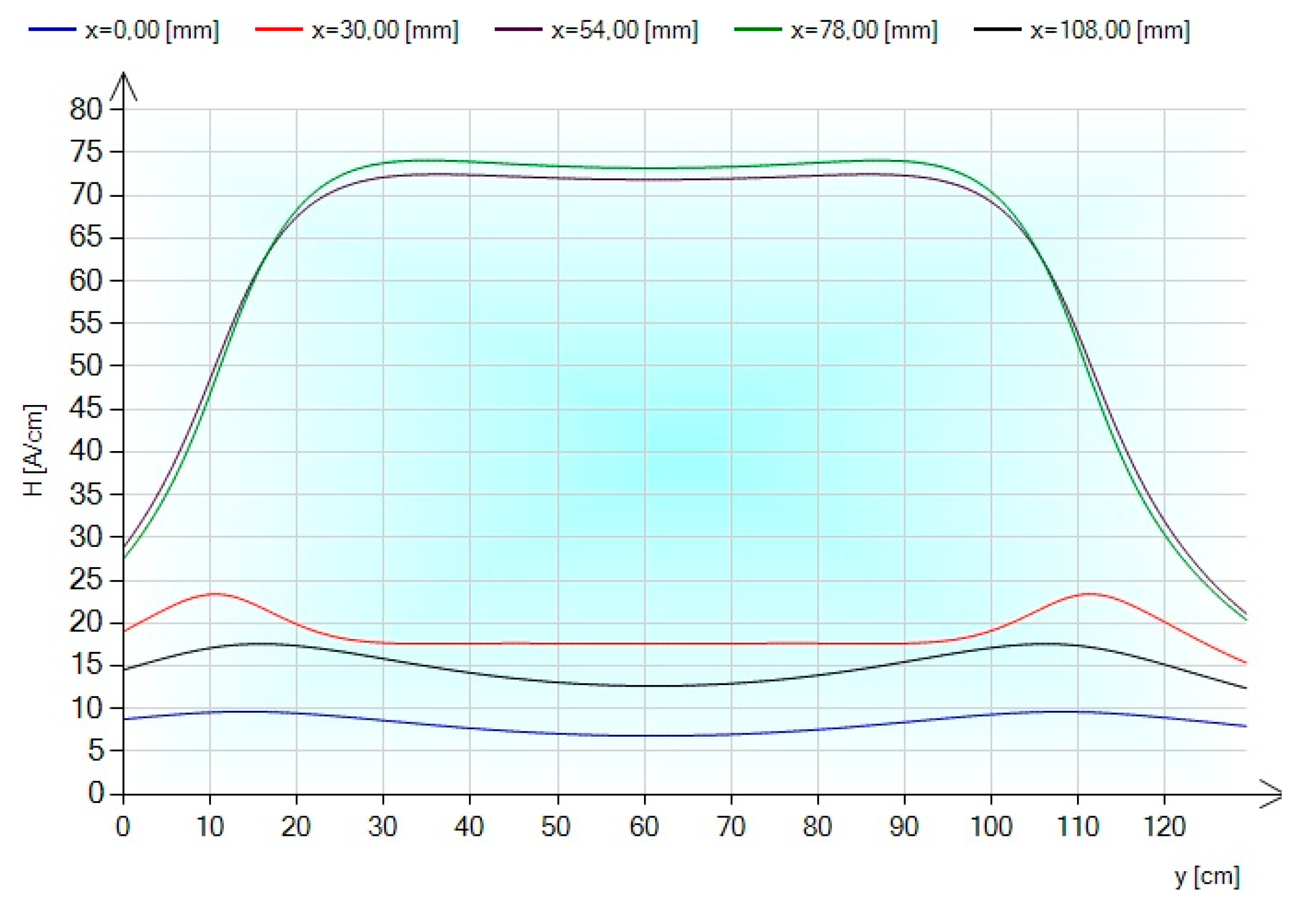
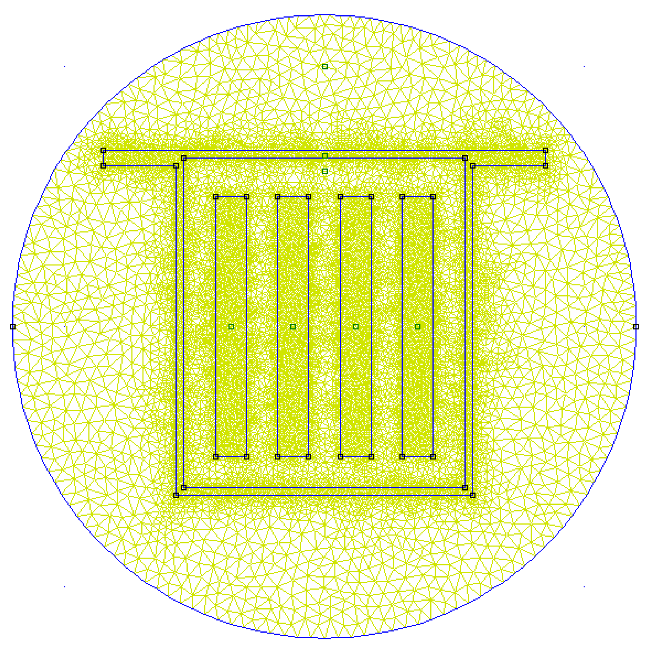
3.2. Magnetic Field of Rectangular Busducts

Knowledge of the current density at individual elementary conductors of busducts allows calculation of the magnetic field distribution. The magnetic field generated by the known current density of such an elementary conductor can be determined by the medium of the vector potential generated by this current in the space [34,35,36]. For the elementary conductor shown in the Figure 8, this potential is given by the formula

$${\underset{\_}{\mathit{A}}}_{i,k}^{(m)}(\mathit{P})=\frac{{\mathsf{\mu }}_0}{4\mathsf{\pi }}{\displaystyle \underset{v_{i,k}^{(m)}}{\iiint }\frac{{\underset{\_}{\mathit{J}}}_{i,k}^{(m)}(\mathit{Q})}{r(\mathit{P},\mathit{Q})}}\mathrm{d}{v}_Q={\mathbf{1}}_z{\underset{\_}{A}}_{i,k}^{(m)}(x,y,z)$$

(43)

With (42), the component of the magnetic vector potential in the direction of Oz axis is given by the formula

$${\underset{\_}{A}}_{i,k}^{(m)}(x,y,z)=\frac{{\mathsf{\mu }}_0}{4\mathsf{\pi }}\frac{{\underset{\_}{I}}_{i,k}^{(m)}}{S_{i,k}^{(m)}}{\displaystyle \underset{0}{\overset{l_{i,k}^{(m)}}{\int }}{\displaystyle \underset{y_{i,k}^{(m)}}{\overset{y_{i,k}^{(m)}+\Delta y_{i,k}^{(m)}}{\int }}{\displaystyle \underset{x_{i,k}^{(m)}}{\overset{x_{i,k}^{(m)}+\Delta x_{i,k}^{(m)}}{\int }}\frac{\mathrm{d}{x}_1\mathrm{d}{y}_1\mathrm{d}{z}_1}{\sqrt{{\left(x-x_1\right)}^2+{\left(y-x_1\right)}^2+{\left(z-x_1\right)}^2}}}}}$$

(44)

If $l_{i,k}^{\left(m\right)}\gg \Delta x_{i,k}^{\left(m\right)}\mathrm{and}{l}_{i,k}^{\left(m\right)}\gg \Delta y_{i,k}^{\left(m\right)}$ and if the point $\mathit{P}\left(x,y,z\right)$ is far enough from element $v_{i,k}^{\left(m\right)}$, ergo $\left|x-x_1\right|\gg \Delta x_{i,k}^{\left(m\right)}$ and $\left|y-y_1\right|\gg \Delta y_{i,k}^{\left(m\right)}$, then the triple integral (44) can be calculated with sufficient accuracy as follows

$${\underset{\_}{A}}_{i,k}^{(m)}(x,y,z)=\frac{{\mathsf{\mu }}_0{\underset{\_}{I}}_{i,k}^{(m)}}{4\mathsf{\pi }}{\displaystyle \underset{0}{\overset{l_{i,k}^{(m)}}{\int }}\frac{\mathrm{d}{z}_1}{\sqrt{{\left(x-x_{i,k}^{(m)}-\frac{1}{2}\Delta x_{i,k}^{(m)}\right)}^2+{\left(y-y_{i,k}^{(m)}-\frac{1}{2}\Delta y_{i,k}^{(m)}\right)}^2+{\left(z-z_1\right)}^2}}}$$

(45)

Knowledge of the vector potential allows determination of the magnetic field strength as

$${\underset{\_}{\mathit{H}}}_{i,k}^{(m)}(x,y,z)=\frac{1}{{\mathsf{\mu }}_0}\mathbf{rot}{\underset{\_}{A}}_{i,k}^{(m)}(x,y,z)={\mathbf{1}}_x\frac{1}{{\mathsf{\mu }}_0}\frac{\partial {\underset{\_}{A}}_{i,k}^{(m)}(x,y,z)}{\partial y}-{\mathbf{1}}_y\frac{1}{{\mathsf{\mu }}_0}\frac{\partial {\underset{\_}{A}}_{i,k}^{(m)}(x,y,z)}{\partial x}$$

(46)

that is

$${\underset{\_}{\mathit{H}}}_{i,k}^{(m)}(x,y,z)={\mathbf{1}}_x{\underset{\_}{H}}_{x,i,k}^{(m)}+{\mathbf{1}}_y{\underset{\_}{H}}_{y,i,k}^{(m)}$$

(47)

where the magnetic field strength components are

$${\underset{\_}{H}}_{x,i,k}^{(m)}=\frac{1}{{\mathsf{\mu }}_0}\frac{\partial {\underset{\_}{A}}_{i,k}^{(m)}(x,y,z)}{\partial y}$$

(48)

and

$${\underset{\_}{H}}_{y,i,k}^{(m)}=-\frac{1}{{\mathsf{\mu }}_0}\frac{\partial {\underset{\_}{A}}_{i,k}^{(m)}(x,y,z)}{\partial x}$$

(49)

Hence, these components are given by the following integrals:

$${\underset{\_}{H}}_{x,i,k}^{(m)}(x,y,z)=\frac{{\underset{\_}{I}}_{i,k}^{(m)}}{4\mathsf{\pi }}{\displaystyle \underset{0}{\overset{l_{i,k}^{(m)}}{\int }}\frac{-\left(y-y_{i,k}^{(m)}-\frac{1}{2}\Delta y_{i,k}^{(m)}\right)\mathrm{d}{z}_1}{{\left[{\left(x-x_{i,k}^{(m)}-\frac{1}{2}\Delta x_{i,k}^{(m)}\right)}^2+{\left(y-y_{i,k}^{(m)}-\frac{1}{2}\Delta y_{i,k}^{(m)}\right)}^2+{\left(z-z_1\right)}^2\right]}^{\frac{3}{2}}}}$$

(50)

and

$${\underset{\_}{H}}_{y,i,k}^{(m)}(x,y,z)=\frac{{\underset{\_}{I}}_{i,k}^{(m)}}{4\mathsf{\pi }}{\displaystyle \underset{0}{\overset{l_{i,k}^{(m)}}{\int }}\frac{\left(x-x_{i,k}^{(m)}-\frac{1}{2}\Delta x_{i,k}^{(m)}\right)\mathrm{d}{z}_1}{{\left[{\left(x-x_{i,k}^{(m)}-\frac{1}{2}\Delta x_{i,k}^{(m)}\right)}^2+{\left(y-y_{i,k}^{(m)}-\frac{1}{2}\Delta y_{i,k}^{(m)}\right)}^2+{\left(z-z_1\right)}^2\right]}^{\frac{3}{2}}}}$$

(51)

The definite integrals (50) and (51) can be calculated by means of standard functions because the adequate indefinite integral $\Im (z,a,b)$, where $\xi =z-z_1$, has the analytic form

$$\Im (z,a,b)={\displaystyle \int \frac{b\mathrm{d}\xi }{{[a^2+b^2+{\xi }^2]}^{3/2}}}=\frac{b}{a^2+b^2}\frac{\xi }{\sqrt{a^2+b^2+{\xi }^2}}$$

(52)

The above solution allows expression of the magnetic field strength components as follows:

$${\underset{\_}{H}}_{x,i,k}^{(m)}(x,y,z)=\frac{{\underset{\_}{I}}_{i,k}^{(m)}}{4\mathsf{\pi }}\left[\begin{array}{l}\Im (z,x-x_{i,k}^{(m)}-\frac{1}{2}\Delta x_{i,k}^{(m)},y-y_{i,k}^{(m)}-\frac{1}{2}\Delta y_{i,k}^{(m)})-\\ \Im (l_{i,k}^{(m)}-z,x-x_{i,k}^{(m)}-\frac{1}{2}\Delta x_{i,k}^{(m)},y-y_{i,k}^{(m)}-\frac{1}{2}\Delta y_{i,k}^{(m)})\end{array}\right]$$

(53)

and

$${\underset{\_}{H}}_{y,i,k}^{(m)}(x,y,z)=-\frac{{\underset{\_}{I}}_{i,k}^{(m)}}{4\mathsf{\pi }}\left[\begin{array}{l}\Im (z,y-y_{i,k}^{(m)}-\frac{1}{2}\Delta y_{i,k}^{(m)},x-x_{i,k}^{(m)}-\frac{1}{2}\Delta x_{i,k}^{(m)})-\\ \Im (l_{i,k}^{(m)}-z,y-y_{i,k}^{(m)}-\frac{1}{2}\Delta y_{i,k}^{(m)},x-x_{i,k}^{(m)}-\frac{1}{2}\Delta x_{i,k}^{(m)})\end{array}\right]$$

(54)

Finally, the total magnetic field in the outside of the busduct will be a superposition of partial fields generated by currents at all elementary conductors, that is

$${\underset{\_}{H}}_x(x,y,z)={\displaystyle \sum _{i=1}^{N_c}{\displaystyle \sum _{k=1}^{N_i}{\displaystyle \sum _{m=1}^{N_{i,k}}{\underset{\_}{H}}_{x,i,k}^{(m)}(X)}}}$$

(55)

and

$${\underset{\_}{H}}_y(x,y,z)={\displaystyle \sum _{i=1}^{N_c}{\displaystyle \sum _{k=1}^{N_i}{\displaystyle \sum _{m=1}^{N_{i,k}}{\underset{\_}{H}}_{y,i,k}^{(m)}(X)}}}$$

(56)

and then

$$\underset{\_}{\mathit{H}}(x,y,z)={\mathbf{1}}_x\underset{\_}{H_x}(x,y,z)+{\mathbf{1}}_y\underset{\_}{H_y}(x,y,z)$$

(57)

In the three-phase busduct system, the magnetic field is elliptical [1,2]. Its instantaneous value is

$$\mathit{H}(x,y,z,t)={\mathbf{1}}_x\sqrt{2}\mathrm{Re}({\underset{\_}{H}}_x{\mathrm{e}}^{j\omega t})+{\mathbf{1}}_y\sqrt{2}\mathrm{Re}({\underset{\_}{H}}_y{\mathrm{e}}^{j\omega t})$$

(58)

The highest value of the magnetic field is then [1,34]

$$H_{\max }(x,y,z)=\underset{0\le t\le T}{\max }\frac{\left|\mathit{H}(x,y,z,t)\right|}{\sqrt{2}}=\left|{\underset{\_}{H}}_1(x,y,z)\right|+\left|{\underset{\_}{H}}_2(x,y,z)\right|$$

(59)

and the lowest value is

$$H_{\min }(x,y,z)=\underset{0\le t\le T}{\min }\frac{\left|\mathit{H}(x,y,z,t)\right|}{\sqrt{2}}=\left|\left|{\underset{\_}{H}}_1(x,y,z)\right|-\left|{\underset{\_}{H}}_2(x,y,z)\right|\right|$$

(60)

where

$${\underset{\_}{H}}_1(x,y,z)=\frac{{\underset{\_}{H}}_x(x,y,z)+\mathrm{j}{\underset{\_}{H}}_y(x,y,z)}{2}$$

(61)

and

$${\underset{\_}{H}}_2(x,y,z)=\frac{{\underset{\_}{H}}_x^{\ast }(x,y,z)+\mathrm{j}{\underset{\_}{H}}_y^{\ast }(x,y,z)}{2}$$

(62)

3.3. Magnetic Field—Measurement and Results

Firstly, the symmetrical currents forcing was assumed

$${\underset{\_}{I}}_1=I{\mathrm{e}}^{{\mathrm{j}0}^{\mathrm{o}}},{\underset{\_}{I}}_2=I{\mathrm{e}}^{-{\mathrm{j}120}^{\mathrm{o}}},{\underset{\_}{I}}_3=I{\mathrm{e}}^{{\mathrm{j}120}^{\mathrm{o}}},{\underset{\_}{I}}_N={\underset{\_}{I}}_1+{\underset{\_}{I}}_2+{\underset{\_}{I}}_3=0$$

(63)

Secondly, by using the analytical method (AM), neglecting the skin and proximity effects, the distribution of the magnetic field intensity for the unshielded busbar—with one bar per phase and one neutral bar—was determined. The relevant graphs from [37] are shown in Figure 9, Figure 10 and Figure 11.

If skin and proximity effects are taken into account, then in order to determine the magnetic field intensity distribution of an unshielded and shielded busbar, the integral equation method (IEM) should be used. The relevant graphs are shown in Figure 12, Figure 13, Figure 14, Figure 15, Figure 16 and Figure 17.

The aforementioned magnetic field intensity distributions were compared with each other along with the results obtained using the analytical method (AM), the integral equation method (IEM), the finite element method (FEM), and the measurement results (meas). The computations were done with FEM (using FEMM software). Figure 16 shows the mesh generated by the software. The comparison was made at selected points of a shielded and unshielded busbar manufactured by Holduct [5]. The locations of the points are illustrated in Figure 17 (with and without enclosure respectively), and the results are presented in

Table 3. Magnetic field intensity (in kA/m) at selected points of an unshielded (u) and shielded (s) three-phase busbar system manufactured by Holduct with current symmetry of I = 1 kA.

	s	Method	Measurement Points
u			1	2	3	4	5	6	7	8	9	10	11	12
u		AM	0.727	1.316	3.112	3.624	5.594	4.050	0.609	0.965	1.467	1.701	1.467	0.929
		IEM	0.550	1.450	3.150	3.250	4.560	4.250	0.600	1.200	1.250	1.850	1.200	0.950
		FEM	1.036	2.118	4.778	5.537	4.966	1.818	0.873	1.439	2.206	2.547	2.238	1.357
		meas	0.318	1.723	4.041	4.422	3.650	1.419	0.754	1.274	2.058	2.296	1.761	1.153
s		IEM	0.550	2.050	2.850	3.250	3.200	0.950	0.490	0.750	1.050	1.100	0.950	0.550
		FEM	1.180	2.823	4.725	4.313	4.464	1.890	0.626	0.908	1.183	1.468	1.406	0.807
		meas	0.729	2.020	3.563	3.534	3.355	1.423	0.535	0.735	0.960	1.240	1.068	0.661

u: unshielded; s: shielded.

.

4. Discussion

The numerical method is validated by the FEM software and laboratory measurements. Skin, proximity, and eddy current effects are taken into consideration. The results from the measurements indicate that the our numerical method can be used to predict impedance of any such rectangular busbar system with a good accuracy. Both busbar and enclosure have a great influence on its impedance. The model predictions are found to be in very good agreement with measurements.

In the 4 × 4 impedance matrix (Table 1), it is necessary to pay attention to the significant differences between the reactances calculated by the IEM and reactances determined by the FEM. This is due to the poor physical interpretation of self and mutual busbar impedances [38,39,40,41,42,43,44]. If the physical significance of these reactances described by a 3 × 3 impedance matrix (Table 2) is considered, then the differences between these reactances calculated by the IEM and FEM practically disappear. However, it is necessary to additionally take into account the fact that in the IEM these reactances are calculated for a finite length busbar, while in the FEM, they are calculated per unit of length (long bars). The measured resistance values are lower than the calculated ones by less than 15% in the case of unshielded busbars and less than 12% in the case of shielded busbars. The measured reactance values are greater than the calculated ones by less than 5% in the case of unshielded busbars and less than 14% in the case of shielded busbars.

The results show that the magnetic field found by computations and measurement (Table 3) roughly agree at most probing points, although at some points the differences are rather large. This may come from difficulties with the exact positioning of the probe. The differences can be also explained by the difficulty to correctly assess the magnetic field interactions far away from their emission points.

5. Conclusions

Based on the theory of electromagnetic fields and electrodynamics, with the use of the integral equation method, analytical formulas were derived to determine the impedances and the magnetic fields of rectangular busbar systems. These formulas apply to rectangular busbars of any cross-sectional dimensions and any length. They take into account the finite transverse dimensions and the finite length of the busbars. They can be used for any values of complex currents, in particular in cases of a three-phase high-current bus.

The values presented in Table 1 and Table 2 show that the impedance values—calculated on the basis of integral equations—are close to the measured values. The relative error does not exceed 10%. The measured levels are slightly higher than those calculated. This is due to the adoption of some simplifications in the shield geometry (Figure 3) and does not take into account the mathematical model of the actual shape of the shield (Figure 16).

In the case of impedance values obtained using the finite element method, they are almost identical to the values calculated on the basis of integral equations.

The designed and constructed lab stand allowed experimental verification of magnetic fields around a power transmission line with rectangular bus bars. The results of computations and measurements roughly agree at most probing points. At some points the differences seem considerable. This is probably the result of inexact positioning of the probe during the experiment, as well as the fact that its head has considerable size in comparison to the gaps between the bus bars. This shows that magnetic field measurements between tightly packed elements are troublesome and require more accurate methods.

References

1. Kusiak, D.; Szczegielniak, T. Electromagnetic Calculations of Busbars; Series Monograph No. 326; Publisher Częstochowa University of Technology: Czestochowa, Poland, 2017; p. 177. (In Polish) [Google Scholar]
2. Piątek, Z. Impedances of Tubular High Current Busducts; Polish Academy of Sciences: Warsaw, Poland, 2008. [Google Scholar]
3. Kusiak, D.; Piątek, Z.; Szczegielniak, T.; Jabłoński, P. Calculations of the magnetic field of the 3-phase, 4-conductor line with rectangular busbar. Comput. Appl. Electr. Eng. 2016, 14, 25–38. (In Polish) [Google Scholar]
4. Sarajčev, P.; Goić, R. Power loss computation in high-current generator busducts of rectangular cross-section. Electr. Power Compon. Syst. 2010, 38, 1469–1485. [Google Scholar]
5. Holduct Ltd. Three-Phase Busduct; Poland. Available online: http://energetyka.holduct.com.pl (accessed on 12 March 2019).
6. Rolicz, P. Skin effect in a system of two rectangular conductors carrying identical currents. Electr. Eng. 2000, 82, 285–290. [Google Scholar] [CrossRef]
7. Capelli, F.; Riba, J.R. Analysis of formulas to calculate the AC inductance of different configurations of nonmagnetic circular conductors. Electr. Eng. 2017, 99, 827–837. [Google Scholar] [CrossRef]
8. Cai, C.; Xuejun, P.; Yu, C.; Yong, K. Investigation, Evaluation and Optimization of Stray Inductance in Laminated Busbar. IEEE Trans. Power Electron. 2014, 29, 3679–3692. [Google Scholar]
9. Riba, J.R.; Capelli, F. Calculation of the inductance of conductive nonmagnetic conductors by means of finite element method simulations. Int. J. Electr. Educ. 2018, 1–23. [Google Scholar] [CrossRef]
10. Benato, R.; Dughiero, F.; Forzan, M.; Paolucci, A. Proximity effect and magnetic field calculation in GIL and in isolated phase busducts. IEEE Trans. Magn. 2002, 2, 781–784. [Google Scholar] [CrossRef]
11. Piątek, Z. Self and mutual impedances of a finite length gas insulated transmission line (GIL). Electr. Power Syst. Res. 2007, 77, 191–203. [Google Scholar] [CrossRef]
12. Piatek, Z.; Kusiak, D.; Szczegielniak, T. Electromagnetic Field and Impedances of High Current Busducts. In Proceedings of the International Symposium Modern Electric Power Systems (MEPS), Wroclaw, Poland, 20–22 September 2010. [Google Scholar]
13. Lovrić, D.; Boras, V.; Vujević, S. Accuracy of approximate formulas for internal impedance of tubular cylindrical conductors for large parameters. Prog. Electromagn. Res. M 2011, 16, 171–184. [Google Scholar] [CrossRef]
14. Fazljoo, S.A.; Besmi, M.R. A new method for calculation of impedance in various frequencies. In Proceedings of the 1st Power Electronic & Drive Systems & Technologies Conference(PEDSTC), Tehran, Iran, 17–18 February 2010; pp. 36–40. [Google Scholar]
15. Goddard, K.F.; Roy, A.A.; Sykulski, J.K. Inductance and resistance calculations for a pair of rectangular conductor. IEE Proc. Sci. Meas. Technol. 2005, 152, 73–78. [Google Scholar] [CrossRef]
16. Xinglong, Z.; Baichao, C.; Yao, L.; Runhang, Z. Analytical Calculation of Mutual Inductance of Finite-Length Coaxial Helical Filaments and Tape Coils. Energies 2019, 12, 20. [Google Scholar]
17. Aebischer, H.A.; Friedli, H. Analytical approximation for the inductance of circularly cylindrical two-wire transmission lines with proximity effect. Adv. Electromagn. 2018, 7, 25–34. [Google Scholar] [CrossRef]
18. Piątek, Z.; Baron, B.; Jabłoński, P.; Kusiak, D.; Szczegielniak, T. Numerical method of computing impedances in shielded and unshielded three-phase rectangular busbar systems. Prog. Electromagn. Res. B 2013, 51, 135–156. [Google Scholar] [CrossRef]
19. Sarajčev, P. Numerical analysis of the magnetic field of high-current busduct and GIL systems. Energies 2011, 4, 2196–2211. [Google Scholar] [CrossRef]
20. Koch, H. Gas-Insulated Transmission Lines (GIL); John Wiley&Sons: Hoboken, NJ, USA, 2012. [Google Scholar]
21. Koch, H.; Benato, R.; Laußegger, M.; Köhler, M.; Leung, K.K.; Mirebeau, P.; Kindersberger, J.; Kunze, D.; di Mario, C.; Renaud, F.; et al. Application of long high capacity gas-insulated lines in structures. IEEE Trans. Power Deliv. 2007, 22, 619–626. [Google Scholar]
22. Völcker, O.; Koch, H. Insulation co-ordination for gas-insulated transmission lines (GIL). IEEE Trans. Power Deliv. 2001, 16, 122–130. [Google Scholar] [CrossRef]
23. Piątek, Z.; Baron, B.; Szczegielniak, T.; Kusiak, D.; Pasierbek, A. Numerical method of computing impedances of a three-phase busbar system of rectangular cross section. Prz. Elektrotech. 2013, 89, 150–154. [Google Scholar]
24. Piątek, Z.; Baron, B.; Szczegielniak, T.; Kusiak, D.; Pasierbek, A. Exact closed form formula for mutual inductance of conductors of rectangular cross section. Prz. Elektrotech. 2013, 89, 61–64. [Google Scholar]
25. Piątek, Z.; Baron, B.; Szczegielniak, T.; Kusiak, D.; Pasierbek, A. Inductance of along two-rectangular busbar single-phase line. Prz. Elektrotech. 2013, 89, 290–292. [Google Scholar]
26. Piątek, Z.; Baron, B.; Szczegielniak, T.; Kusiak, D.; Pasierbek, A. Mutual inductance of two thin tapes with parallel widths. Prz. Elektrotech. 2013, 89, 281–283. [Google Scholar]
27. Piątek, Z.; Baron, B.; Szczegielniak, T.; Kusiak, D.; Pasierbek, A. Mutual inductance of two thin tapes with perpendicular widths. Prz. Elektrotech. 2013, 89, 287–289. [Google Scholar]
28. Szczegielniak, T.; Piątek, Z.; Kusiak, D.; Kusiak, D. Self and mutual impedances of rectangular bus-bars of finite length. Inform. Autom. Pomiary Gospod. Ochr. Śr. (IAPGOŚ) 2014, 4, 21–24. (In Polish) [Google Scholar]
29. Piątek, Z.; Baron, B. Exact closed form formula for self inductance of conductor of rectangular cross section. Prog. Electromagn. Res. M 2012, 26, 225–236. [Google Scholar] [CrossRef]
30. Piątek, Z.; Baron, B.; Jabłoński, P.; Szczegielniak, T.; Kusiak, D.; Pasierbek, A. A numerical method for current density determination in three-phase bus-bars of rectangular cross section. Prz. Elektrotech. 2013, 89, 294–298. [Google Scholar]
31. Baron, B.; Piątek, Z.; Szczegielniak, T.; Kusiak, D.; Pasierbek, A. Impedance of an isolated rectangular conductor. Prz. Elektrotech. 2013, 89, 278–280. [Google Scholar]
32. Meeker, D.C. Finite Element Method Magnetics, Version 4.2. 25 October 2015. Available online: http://www.femm.info (accessed on 17 March 2019).
33. Labridis, D.; Hatziathanassiou, V. Finite Element Computation of Field, Forces and Inductances in Underground SF6 Insulated Cables Using a Coupled Magneto-Thermal Formulation. IEEE Trans. Magn. 1994, 4, 1407–1415. [Google Scholar] [CrossRef]
34. Krakowski, M. Theoretical Electrotechnics. Electromagnetic Field, 5th ed.; WN PWN: Warsaw, Poland, 1995. (In Polish) [Google Scholar]
35. Piątek, Z.; Jabłoński, P. Basics of Electromagnetic Field Theory; WNT: Warszawa, Poland, 2010. (In Polish) [Google Scholar]
36. Kazimierczuk, M.K. High-Frequency Magnetic Components; J Wiley&Sons: Chichester, UK, 2009. [Google Scholar]
37. Gliński, H.; Grzymkowski, R.; Kapusta, A.; Słota, D. Mathematica 8; Wyd. Skalmierskiego: Gliwice, Poland, 2012. (In Polish) [Google Scholar]
38. Broydé, F.; Clavelier, E.; Broydé, L. A direct current per-unit-length inductance matrix computation using modified partial inductance. In Proceedings of the CEM 2012 International Symposium on Electromagnetic Compatibility, Rouen, France, 25–27 April 2012. [Google Scholar]
39. Paul, C.R. Inductance: Loop and Partial; J Wiley&Sons: Hoboken, NJ, USA, 2010. [Google Scholar]
40. Paul, C.R. Analysis of Multiconductor Transmission Lines; J Wiley&Sons: Hoboken, NJ, USA, 2010. [Google Scholar]
41. Clavel, E.; Roudet, J.; Foggia, A. Electrical modeling of transformer connecting bars. IEEE Trans. Magn. 2002, 38, 1378–1382. [Google Scholar] [CrossRef]
42. Zhihua, Z.; Weiming, M. AC impedance of an isolated flat conductor. IEEE Trans. Electromagn. Compat. 2002, 44, 482–486. [Google Scholar] [CrossRef]
43. Matsuki, M.; Matsushima, A. Improved numerical method for computing internal impedance of a rectangular conductor and discussions of its high frequency behavior. Prog. Electromagn. Res. M 2012, 23, 139–152. [Google Scholar] [CrossRef]
44. Jabłoński, P.; Kusiak, D.; Szczegielniak, T.; Piątek, Z. Reduction of Impedance Matrices of Power Busducts. Prz. Elektrotech. 2016, 92, 49–52. [Google Scholar]
Figure 1. Three phase bus duct with a neutral busbar manufactured by the Holduct company (Myslowice, Poland) [5].
Energies 12 01419 g001
Figure 2. Unshielded bus duct manufactured by the Holduct company [5].
Energies 12 01419 g002
Figure 3. Shielded bus duct manufactured by the Holduct company [5].
Energies 12 01419 g003
Figure 4. Electric circuit model of high-current busduct with current Ii in a closed loop i-N and impedances Zii and Zij.
Energies 12 01419 g004
Figure 5. Electric circuit model of a high-current busduct with current I2 in a closed loop 2-N and reduced self-impedances zii and mutual impedances zij.
Energies 12 01419 g005
Figure 6. Circuit model of a high-current bus duct with a division of phase busbars, a neutral busbar, and a shield into elementary conductors in the case of shield grounding at its ends.
Energies 12 01419 g006
Figure 7. Measurement stand: 1—busbar manufactured by the Holduct company [5], 2—shield cover, 3—current transformer, 4—Rogowski coils, 5—voltmeter, 6—phase meter, 7—PC with measurement software.
Energies 12 01419 g007
Figure 8. Location v i , k ( m ) of the m-th elementary conductor of the i-th phase of the k-th conductor.
Energies 12 01419 g008
Figure 9. The distribution of magnetic field intensity along the line y = const (constants) of an unshielded busbar system with current symmetry.
Energies 12 01419 g009
Figure 10. The distribution of magnetic field intensity along the line x = const of an unshielded busbar system with current symmetry.
Energies 12 01419 g010
Figure 11. Spatial distribution of magnetic field intensity of an unshielded busbar system with current symmetry.
Energies 12 01419 g011
Figure 12. The distribution of magnetic field intensity of an unshielded busbar system for x = var (variables) and different values of y = const in the case of current symmetry.
Energies 12 01419 g012
Figure 13. The distribution of magnetic field intensity of a shielded busbar system for x= var and different values of y = const in the case of current symmetry.
Energies 12 01419 g013
Figure 14. The distribution of magnetic field intensity of an unshielded busbar system for y = var and different values of x = const in the case of current symmetry.
Energies 12 01419 g014
Figure 15. The distribution of magnetic field intensity of a shielded busbar system for y = var and different values of x = const in the case of current symmetry.
Energies 12 01419 g015
Figure 16. The cross-section of busbar system (shielded)with finite element method (FEM) mesh.
Energies 12 01419 g016
Figure 17. The location of measurement points of a shielded (unshielded) busbar system.
Energies 12 01419 g017