Abstract
In March 2016, arguably the most ambitious 4D (3D space + over time) active-source seismic survey for geothermal exploration in the U.S. was acquired at Brady Natural Laboratory, outside Fernley, Nevada. The four-week experiment included 191 vibroseis source locations, and approximately 130 m of distributed acoustic sensing (DAS) in a vertical well, located at the southern end of the survey area. The imaging of the geothermal faults is done with reverse time migration of the DAS data for both P-P and P-S events in order to generate 3D models of reflectivity, which can identify subsurface fault locations. Three scenarios of receiver data are explored to investigate the reliability of the reflectivity models obtained: (1) Migration of synthetic P-P and P-S DAS data, (2) migration of the observed field DAS data and (3) migration of pure random noise to better assess the validity of our results. The comparisons of the 3D reflectivity models from these three scenarios confirm that sections of three known faults at Brady produce reflected energy observed by the DAS. Two faults that are imaged are ~1 km away from the DAS well; one of these faults (middle west-dipping) is well-constructed for over 400 m along the fault’s strike, and 300 m in depth. These results confirm that the DAS data, together with an imaging engine such as reverse time migration, can be used to position important geothermal features such as faults.
1. Introduction
Geophysical data can provide some of the most spatially extensive information about the subsurface, and has a long and successful exploration role in the oil and gas industry [1,2]. Seismic data, which utilizes elastic waves and how they reflect and refract off of materials with contrasting density and elastic moduli, has provided incredibly detailed models of faults, salt diapers and other important geologic features at depths reaching 100 km. Analogous to medical imaging technologies such as Ultrasound or magnetic resonance imaging (MRI) scans, which probe the structure of our body using physical fields, geophysical sensors (such as geophones or DAS sensors), are often placed at the surface, and measure physical fields, specifically in this paper, elastic waves. Like the ultrasound which probes the body with ultrasonic waves, active seismic sources such as dynamite explosions, vibroseis trucks or hammer swings, induce seismic waves probing the subsurface at increasing depths. Figure 1 depicts an incident primary wave, which is induced by a vibroseis source (the truck on the ground surface), and two possible reflected waves: P (primary-compressional) and S (shear) waves. The reflections occur because of changes in material properties such as density (ρ) and the acoustic velocities (Vp and Vs), according to Snell’s law [3].
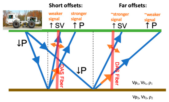
Figure 1.
Schematic of an incident P (primary) wave (from a vibroseis truck), and the resulting reflected P (primary) and S (shear) Vertical (SV) waves for short (left) and far (right) offsets. Primary waves have the same propagation (blue arrows) and particle (orange arrows) motion direction, whereas S waves’ particle direction (orange arrow) is perpendicular to the propagation direction (blue arrows).
Geologic faults can provide abrupt changes in material properties, thus generating reflections and diffractions that can be recorded by seismological sensors. For geothermal applications, seismic methods have been used to locate faults, which will in turn help optimize the placement of future production wells, as faults can act as conduits for hot fluids to reach accessible depths [4]. Melosh et al. [5] describe the challenges of coherent noise masquerading as fault signatures in reflection seismic studies at the Blue Mountain geothermal field. However, recently, Huang et al. [6] describe a state of the art anisotropic 2D migration technique applied to Blue Mountain, which revealed previously unseen faults from the traditional Kirchhoff approach.
Faults provide one of the principal means for a recharge of the geothermal reservoirs, particularly in the Basin and Range Region of Nevada, USA [7]. The faults of Brady Hot Springs (located near Fernley, NV, USA) have been studied extensively [8,9,10], as it is interpreted that they have allowed the near-continuous power production since 1991 via the recharge of water from the surface or re-injection [11]. Previous analysis from InSAR and pumping data have hypothesized that the faults act as highly permeable conduits, which channel fluids from shallow aquifers to the deep geothermal reservoir tapped by the production wells [12].
In particular, Siler and Faulds [10] provided a 3D numerical fault model for the Brady system by integrating legacy 2D seismic reflection data, downhole lithologic data, and geologic map data. As stated in [10], Brady is controlled by a step-over normal fault system, and the area contains active fumaroles, sinter, calcium carbonate tufa and silicified sediments. The authors refer readers to [10] for an in-depth geologic review. Some of the faults are interpreted to have up to 10 m of displacement, and could thus provide reflections [13]. Figure 2 displays the four major faults from the Siler & Faulds model. A study by Queen et al. [13] concluded that vertical seismic profiling would be more successful than surface sensors at imaging the nearly vertical faults expected at Brady, and depicted in the Siler & Faulds model. Our results confirm the findings of the Queen et al. work.
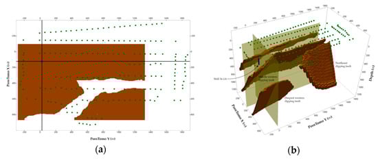
Figure 2.
(a) Map view of survey: Well 56-1A in blue near PoroTomo origin (location of vertical distributed acoustic sensing (DAS)) and surface sources shown in green dots. (b) Southern view of 3D rendering of four faults model [10]. The three faults successfully imaged are labeled middle & deepest Western dipping fault on the left, and the Northeast dipping fault on the right.
In March 2016, a four-week experiment known as PoroTomo deployed an integrated technology in a 1500-by-500-by-400-m volume at Brady Hot Springs [14]. The sensors and sources that are of interest for this paper are shown in Figure 2. The 191 active vibroseis locations (known as “vibe points”) are shown as green dots, and the position of Well 56-1A, which contains the vertical fiber-optic cable for the Distributed Acoustic Sensing (DAS), is in blue. The DAS fiber is located from the surface to a depth of approximately 400 m.
The local PoroTomo coordinate system, seen in Figure 2, is chosen such that the Y axis is oriented along the major fault strikes, and the origin of this local system is close to the location of Well 56-1A. Note the three labeled faults in Figure 2 that we will image and compare using the synthetic and DAS field data in the Results Section.
DAS is a novel new type of seismic data, thanks to a combination of fiber-optic cable and advances in optical, light-pulse technology [15]. Traditionally, seismic data is recorded by geophones or seismometers, which are coupled to the ground through spikes, and measure particle acceleration via voltmeters. Instead, DAS uses Rayleigh scattering in a fiber-optic cable to detect changes in strain rate due to seismic waves impinging on the fiber [16,17]. DAS is most sensitive to waves that have particle motion parallel to the orientation of the fiber; DAS is insensitive to particle motion perpendicular to the fiber orientation (referred to as broadside insensitivity). Figure 1 nominally depicts how a vertically-deployed DAS system may be more sensitive to certain reflected waves due to a horizontal reflector. In this simplified case, at short offsets (smaller distances between the source and the vertical DAS, shown on the left side) the vertical DAS will be more sensitive to reflected P-waves rather than S-waves (or specifically SV-wave: shear-waves with particle motion in the vertical direction) because the particle direction (orange arrows) is inline with the fiber. DAS sensitivity may switch to be higher for reflected S-waves at larger offsets, loosely depicted on the right side of Figure 1.
Recently, distributed acoustic sensing (DAS) has been used in the oil and gas industry along with and in place of geophones, as it provides denser spatial sampling than geophones [18,19]. Countering the increased spatial resolution, however, is DAS’s lower signal-to-noise ratio, due to imperfect fiber-subsurface coupling and the directionality sensitivity, with the highest sensitivity to particle motion parallel to the fiber direction. The coupling of the fiber downhole can vary depending upon whether the fiber is installed behind casing or in tubing [20]. This will directly affect the quality of signal measured by the fiber, and whether or not it is representative of the response of the surrounding geologic material.
The DAS research has largely focused on borehole environments in the oil and gas industry, because many wells are already equipped with fiber for monitoring production via other tools; therefore, vertical seismic profiles recorded by DAS are becoming more common place [21]. Many studies focus on how the DAS measurements compare to raw observations with geophones [19,22]. In the borehole environment, as depicted in Figure 1, with approximately horizontal reflectors and relatively close distances between the vibroseis source and the well instrumented with DAS, reflected P-waves will provide particle motion in the vertical direction, thus parallel to the fiber. This will ensure recorded seismic DAS data that contains information about subsurface structure.
Three main challenges exist for the Brady DAS data. First, the fiber itself is not attached to the Well 56-1A infrastructure. This would have required a large investment in the well, such as removing or replacing the existing well casing. Second, the faults of Brady are not horizontal (Figure 2), therefore the reflected waves will result in more complicated and varied particle directions. Lastly, the location of the Well 56-1A is in the extreme southwestern corner of the PoroTomo grid. The quality of the DAS signal will depend on the location of the vibe point, the angle of incidence with the fault, and the type of reflected wave (P- or S-wave). A more ideal acquisition geometry would have the DAS fiber centered among the source locations (e.g., vibe points), allowing for more recordings of the reflected energy. Permitting issues on historical sites and steam sinters were among the top considerations for how the PoroTomo survey was designed [11].
Despite these challenges, the DAS data recorded a sufficient signal that allowed for 3D spatial models to be reconstructed. This paper will describe advanced imaging methods, not historically utilized for geothermal exploration, but popular in the oil and gas industry, that convert the DAS data into 3D reflectivity models that are consistent with the Siler & Faulds fault model. Specifically the reverse-time migration (RTM) method is described and applied to both synthetic and observed DAS data from Brady [23,24]. RTM simulates the propagation of wavefields in 3D space, which is an improvement over traditional seismic modeling techniques that simplify the wave propagation via straight ray paths (as depicted in Figure 1).
Two novel advances for geothermal exploration are presented in this paper. The first contribution is the application and verification of the DAS data to record useful seismic information, despite the challenging scenario at Brady. Second, this paper represents one of the first imaging experiments performed on DAS data, and the first for geothermal applications. The paper will first describe the DAS data and the method of reverse time migration (RTM). The next section will describe the results, which compare imaging using three different receiver wavefields: (1) Synthetic, (2) the DAS data from Brady and (3) pure noise. By comparing these results, we conclude which faults are likely “seen” by the DAS data, and we discuss the significance and possible improvements of this work.
2. Materials and Methods
The data presented in this paper is available either on the PoroTomo data repository or Geothermal Technologies Office Geothermal Data Repository. The numerical imaging experiments utilized the open source code of SepLib [25].
2.1. The Data: Distributed Acoustic Sensing at Brady
The tri-axial vibroseis “T-Rex” from the University of Texas-Austin was utilized for the March 2016 PoroTomo field acquisition. At each vibe location shown in Figure 2a, three repeated sweeps were recorded for each of the three shaking modes. Each 20 s, a linear-sweep injected frequencies of 5–80 Hz into the subsurface. Figure 2a shows the directivity of the in-line and cross-line shear modes. However, for this study, we have only utilized stacked versions of the three vertical (P) sweeps for 191 vibe points. Silixa’s iDASTM was utilized for distributed acoustic sensing (DAS) acquisition with 1 kHz temporal sampling, 0.25 m channel spacing (decimated to 1 m in post-processing), and a gauge length of 10 m [26]. The fiber down the well is composed of a double-stainless steel tube cable with hydrogen scavenging gel and 150 °C harsh environment fibers.
Figure 3 shows examples of the DAS data from two different vibe points (vibe locations 125 and 199) that are at equivalent offset: ~250 m distance between the vibroseis truck and Well 56-1A). The differences in the two DAS profiles demonstrate the azimuthal heterogeneity of the subsurface (they differ by 180 degrees azimuthally). The data display the receiver positions (e.g., DAS sensor locations) in depth on the x-axis and time on the y-axis. In this view, the downgoing waves have a negative slope, propagating at deeper depths at later times, whereas the upgoing waves have a positive slope. In general, Figure 3 is displaying moveout: which is the difference in the arrival times or travel times of waves measured by the DAS sensors (receivers) at different depth locations. While the DAS cables extend from the surface to a depth of 400 m, we only use seismic events recorded between 160 m and 300 m due to noise (reverberations of the steel casing in the shallow part) and attenuation (low amplitude signal).

Figure 3.
DAS data for vibe shots (a) 199 and (b) 125, approximately 150 m away from the well but with azimuths 180° apart.
Figure 3a displays a seismic record for vibe point 199 which is located 256 m to the southwest of Well 56-1A. Figure 3b shows vibe point 125, located about 257 m to the northwest of Well 56-1A. Vibe point 199 in Figure 3a illustrates a downgoing P-wave (highlighted in pink), and a weaker upgoing (reflected and converted) s-wave (highlighted in green). Figure 3b (vibe point 125) also shows a down-going p-wave (pink) and an upgoing s-wave (green), which have stronger amplitudes than in vibe point 199. The upgoing S-wave is much slower in vibe point 125 (Figure 3b) than in 199 (Figure 3a), which is evidence of the heterogeneity in the Brady reservoir.
The downgoing P to upgoing S-wave is an example of a mode conversions: where one type of wave changes to another, which is visually seen as a change in polarity (white-to-dark or vice versa). Figure 1 depicts mode conversions, and there are more subtle examples throughout Figure 3a,b which will contain information about which subsurface features are causing these moveouts.
This paper describes the methods used to probe the DAS data in order to directly image Brady’s important faults. The DAS data is ripe with mode conversions (Figure 3). For the imaging of the faults, we use the reverse time migration technique (explained below) and the Siler & Faulds’ fault model [10] as reflectivity, to begin to explain the DAS signals in terms of the geothermal reservoir faulting.
2.2. Seismic Imaging with Reverse Time Migration
Migration algorithms construct spatial models of reflectivity from seismic observations. In other words, they attempt to place in 2D or 3D space the reflectors that created the observed seismic data. This paper explores how reliably the Brady DAS data can be converted into information about the fault positions in the subsurface (Figure 2). Here we describe the imaging method used for our synthetic and field DAS data. All migrations are performed on a 3D grid with dimensions nx (PoroTomoY) = 322, ny (PoroTomoX) = 193, and nz = 301 (depth), such that each cell represents 5 m in all three dimensions. Migrations were performed using frequencies between 8 Hz and 80 Hz to mimic the field acquisition sweep range.
All migration algorithms (reverse time migration here) image single scattering events, either reflections or diffractions. These algorithms are based on the Born approximation, which decomposes the medium into a background model responsible for travel time (i.e., velocity), and a perturbation model responsible for the reflections and diffractions (i.e., reflectivity) [27].
Therefore, starting from the acoustic wave equation, the Born approximation creates a linear relationship between the seismic data and the reflectivity model obtained with migration, assuming that the seismic data are single-scattered events. Theoretically, with a dense and large grid of sources and receivers, there is enough azimuthal and angle coverage to see diffractions and reflections coming from a wide range of directions.
Often ray paths are used to approximate how seismic energy propagates and samples the subsurface, but there are shortcomings to this approximation: They don’t account for complex multi-pathing, or scattering at locations of high contrast between physical properties. In contrast, wave-equation migration-based methods use the full seismic wavefield, and can handle very high velocity contrasts accurately. Such methods have high computational cost that limits their applicability, but advances in computer hardware and software allow for fast processing of large volumes of data, making such methods feasible. The acoustic wave equation (partial differential equation with constant density) can be used to describe approximately the propagation of seismic waves in subsurface media. The 3D acoustic wave equation is given by
where v, p, t and f are the medium velocity (a function of x, y, z), the scalar wave field, time, and the source term, respectively, and x, y, z are spatial coordinates. Acoustic migration (simulating pressure p) is used in this work, not elastic migration, which simulates displacement. The reflections (P to P and P to S) are kinematically created by simulating their moveout only (while not honoring their elastic amplitudes).
The migration used in this work is a prestack depth migration algorithm called reverse time migration, or RTM for short. RTM is based on the imaging principle of Claerbout [23], where a reflector exists when source and receiver wavefields coincide in space at zero time. A pre-stack depth migration code using the whole wavefield for each source and all receiver positions will give an accurate image of the subsurface if the velocity is accurate enough and reflections and/or diffractions are recorded.
RTM migrates shot gathers, and uses all offsets available (from all receiver positions for a given shot): A source wavefield, Ws, is propagated forward in time in the computational volume, and the observed or synthetic data (the receiver wavefield, Wr) are backward-propagated in time in the same volume. Both wavefields are then multiplied at each time step t, and summed across all time steps to form the final image R as follows:
where x is a vector of spatial coordinates and i the shot index. Amplitudes are not preserved, as the final image represents the zero-lag cross correlation between the source and receiver wavefields. Each gather produces one partial image that is summed to all the other images (coming from all the other shots) to yield the final image. This process is called a “shot profile” algorithm, because it migrates shot gathers individually before summation across shot positions. The image R is then divided by a source illumination map I(x) computed as follows:
This illumination map describes how well the 3D subsurface is explored by the energy of the vibe points [24]. Illumination-compensated images
increase the reflectivity R where illumination I is low, boosting deeper events (reflectors). prevents RIC equal to infinity, where I(x) equals 0, and is usually chosen as a percentile of the illumination map I(x). Finally, a 3D Laplacian filter is applied to the image to remove low-wavenumber artifacts commonly found with RTM (due to backscattering energy correlating in Equation (2) at all positions and all times).
Migration algorithms and results are highly influenced by the velocity model used. Imaging is best performed with body waves which are generated by the vibroseis truck. We use P-wave (Vp) and S-wave (Vs) velocities estimated from sweep interferometry recorded during the March 2016 experiment to image converted-wave reflections generated by the vertical vibrator (assuming a P-wave source) [28]. Figure 4 displays this Vp or P-wave velocity model that was used for imaging. Most figures in this paper will use the flattened cube convention of Figure 4a, which contains the depth slice (top), inline (bottom left, PoroTomoX constant), and cross-line (bottom right, PoroTomoY constant).

Figure 4.
P-Wave Velocity (Vp) model from sweep interferometry [28] with the black lines approximately indicating the location of Well 56-1 at PoroTomoY = 119, PoroTomoX = 24, and depth is 195 m. (a) the flattened cube view with the top the depth slice at 195 m below reference elevation of 1277 m above WGS84 ellipsoid, the lower left the PoroTomoX = 122 slice (inline), the lower right the PoroTomoY = 24 slice (cross-line). (b) is the 3D perspective.
The RTM algorithms used allow for specifying distinct 3D velocity models for the downward going waves versus the upward going waves. The downward going wave should represent the type of source waves induced by the vibroseis. The vibroseis for the PoroTomo experiment are excited by P-source, shear-horizontal, and shear-transverse, however for this study we have only utilized P-source observations. The upgoing velocity model is used for energy that is reflected: either P to P reflections or P to S reflections. To capture both types of wave that can be reflected, both P–P images (P velocity model for both downward and upgoing waves) and P–S images (P velocity model for downward and S velocity for upgoing waves) are generated. The S velocity model used for these numerical experiments demonstrated similar patterns seen in Figure 4, but is on average 1.8 times slower than Vp. As depicted in Figure 1, the angle of incidence is one of the determining factors of whichever types of waves are reflected.
2.3. Synthetic Data Generation with a Born Modeling Approach
We now briefly describe our modeling approach to create synthetic seismic data for the Brady field. The RTM technique described above is the adjoint process of Born modeling. For one shot at a time, Born modeling generates single-scattered reflected events by (1) propagating a source wavefield Ws forward in time (similar to RTM); (2) multiplying this source wavefield at all time steps and x positions with a reflectivity model (i.e., our fault model); and (3) recording the resulting upgoing wavefield Wr at the receiver locations.
Here we simulate the source wavefield Ws to mimic the vibroseis parameters during the March 2016 data acquisition at Brady. We then record the receiver wavefield Wr (reflected signals) at the DAS receiver locations. Figure 5a shows these synthetic observations of the synthetic Wr (upgoing only) for vibe point 125; Figure 5b is the observed field data (observed Wr) for vibe point 125 (same as seen in Figure 3b except now it is filtered to only have upgoing events). Born modeling only models single scattering events [27]. In Figure 5b, the converted upgoing S-wave is quite clearly observed (green line) as the relative moveout contrasts from that of the P-wave first arrival. For this reason, the shear wave velocity was also used for upgoing waves, hence the notation P-S data. The synthetic data follow the observed data where two events travel from the bottom up to 160 m depth, arriving at approximately 0.25 s and 0.4 s respectively (highlighted in yellow and green in Figure 5). We can see that our velocity model is possibly faster than the actual Brady subsurface medium, as the green slope is steeper and arrives earlier in Figure 5a versus Figure 5b.
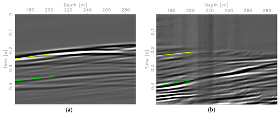
Figure 5.
Vibe point 125: (a) synthetic P-S data via Born approximation/modeling and reflectivity of the 4 faults model [10] and (b) observed data filtered for only upgoing events (same as in Figure 3b).
3. Imaging Results of PP and PS Waves with RTM
This section describes the imaging results of the faults of Brady Hot Springs. Recall that faults are incredibly important structures that indicate locations of recharge and ideal production well sites for geothermal reservoirs. To understand the limitations of imaging, given the Brady’s acquisition geometry, several numerical experiments of synthetic data are generated, and then migrated to isolate our geometry limitations from noise sources and poor coupling. Noise in the data (ground roll, statics/near surface problems, ambient noise, etc.) and an erroneous velocity model, will affect the migration results. Also, if the data coverage is not adequate, resulting in a poor illumination of the subsurface, migrated images will be affected as well. Synthetic modeling allows for both analyzing if the acquisition geometry allows for illumination of the major faults and events of interest, and comparison with the migration of the true field data. First, we start with horizontal reflections, then the steeply dipping faults of the Siler & Faulds fault model are explored and compared with images from the recorded data.
3.1. Estimating Illumination Volume: Four Horizontal Reflectors
The first synthetic test consists of four horizontal reflectors (two constant velocity layers) that extend at depths 750 m, 900 m, 1150 m and 1300 m respectively (see Figure 6b) to demonstrate how much of the image is reliable, given the reflection-point illumination coverage (where illumination describes the degree to which the source energy explores the model space, see Equation (3)). Given the geometry of the sources, certain areas will not be probed by the vibe energy, and thus migration artifacts will dominate. The current velocity model for the area (Figure 4) will also affect the image, and therefore is used in this modeling exercise.
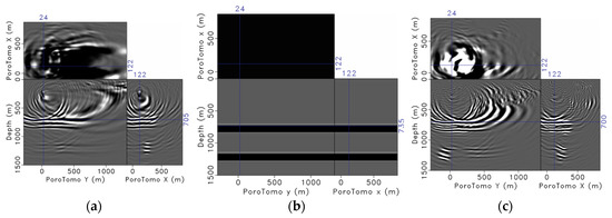
Figure 6.
Reverse-time migration (RTM) result from two flat layers (four reflectors) at 700 m and 1100 m depth. (a) P–P imaging, (b) the reflectivity model used in RTM and (c) P–S imaging.
The observed DAS data (Wr = DAS, Figure 5b) is indeed both noisier (fiber is not adhered to casing) and is picking up on more scattering events than the simulated data (Wr = synthetic. Figure 5a).
Figure 6 contains the two RTM images (a and c) and the model containing the 4 reflectors (b). Figure 6a is the imaging result using the p-wave velocity for the down and upgoing, referred to as the P–P image. Figure 6c is the imaging result using the p-wave velocity for the down-going energy and the shear-wave velocity for the upgoing, referred to as the P–S image. RTM images are composed of a relative reflectivity, where both white and black are stronger magnitudes in images presented here. Experienced interpreters look for and identify coherent structures or events in these images. For example, in Figure 6a,c we see the horizontal reflectors at locations that straddle the well location (about +/−400 m in Y and +/−300 m in X). Beyond this, the image “structure” changes to a “migration smile” indicating poor illumination in that location of the model in these areas.
Thus, given the approximately 130 m of reliable fiber in the well and the vibe point geometry, an 800 m (PoroTomoY) by 600 m (PoroTomoX) by 500 m (depth) volume can successfully recover the four horizontal reflectors. The depth cross section (Figure 6a) shows how the most sensitivity is northeast of the well: The larger swath of darker color in the depth slice (top) indicates the qualitative reflectivity (image) divided by the illumination (Equation (4)). These results indicate that a doublet (reflection from the contrast of both the top and bottom of the reflectors) may be observed. Imaging with P–S events in Figure 6c reduces the illumination in the depth slice (slower S-waves have a lower reflection angle), but it appears to increase the recovery of the deeper flat reflector (at 1100 m depth). Thus, this final reflectivity model indicates a general volume where we can trust features to be possible subsurface structure, and not migration artifacts.
3.2. Comparison of Imaging with Brady DAS Observations and Data Generated with Siler and Faulds Fault Model
This section contains images produced by migrating both the observed field signals from the vertical DAS fiber and synthetic data, where now the synthetic receiver wavefield (Wr) will be produced using the current fault model of Brady (Figure 2) as a reflectivity contrast to analyze if certain fault dips and strikes would be detectable given the vibe point (source) geometry. Additionally, to elucidate where artifacts may be in the 3D image, a third image is produced using a receiver wavefield (Wr) of pure noise. Thus, in this subsection, three images are generated where the receiver wavefield varies as:
- Wr = Synthetic receiver wavefield generated using the Siler & Faulds fault model as reflectors
- Wr = DAS data from Brady collected in March 2016
- Wr = Pure random (white) noise
Each imaging result will be represented by their respective letter in the succeeding figures.
There are many challenges in the DAS Brady data (b. Wr = DAS): reverberating fiber (as it is not affixed to casing or tubing), multiple interfering events, etc. (Figure 3 and Figure 5b). Ideally, the data would be further processed to isolate events of interest.
Since these data are unprocessed, the migrated images will be noisier and more difficult to interpret than the synthetics. Another factor, which is true of both the synthetic and real data case, is the sparse shot geometry. A denser vibe point coverage would produce cleaner migrated images by stacking out artifacts. However, we can utilize the synthetic modeling results to isolate geometry or velocity effects, and attempt to distinguish migration artifacts from true geologic structures.
As described in the Methods Section, two types of RTM were investigated: P–P (P-wave velocity for both up and downgoing waves), and P–S (P-wave velocity for up and S-wave velocity for down going waves). Upgoing shear waves are important if they cross the vertical DAS at an approximately perpendicular angle, since the DAS fiber is sensitive to vertical particle motion (Figure 1).
The next three subsections will focus on three of the four faults seen in Figure 2:
- The deepest northwest dipping fault
- The middle northwest dipping fault
- The eastern-dipping fault.
3.2.1. Deepest Northwestern Dipping Fault
Figure 7 contains two flattened cubes that used the P–P kinematics to produce the illumination-compensated reflectivity images (RIC, Equation (4)) for locations at PoroTomoY = 124 m, PoroTomoX = 672 m, and depth = 420 m, about 225 m deeper and 560 m northeast from the locations shown in Figure 4. Figure 7a contains the RTM result using the synthetic data (a. Wr = synthetic), while Figure 7b is from the Brady’s field data (b. Wr = DAS). These flattened cubes focus on the deepest of the three northwestern-dipping (negative PoroTomoX direction) faults (Figure 2). The intersection of the slices is approximately Northeast (positive PoroTomoY and PoroTomoX direction) of Well 56-1A. The black structures are the fault intersections from the Siler & Faulds model (Figure 2).
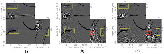
Figure 7.
Deepest West-dipping Fault. Kinematics: P-wave Velocity Down & Up (P–P image) of (a) Wr = synthetic 4 fault model and (b) Wr = Field Brady’s field data (c) Wr = Pure Noise.
The yellow boxes in Figure 7 highlight coherent events that coincide in both the fault model and Brady’s images. All three yellow boxes are on the deepest of the three northwestern-dipping faults. The bottom two slices demonstrate how the fault can be seen from depth ranges of 450–500 m. Additionally, there is a possible coherent event in the Brady’s data that doesn’t coincide with a fault included in the synthetic modeling. This is highlighted in red in the PoroTomoX slice.
Figure 7c contains the image created with c. Wr = Noise; the image emphasizes where artifacts are because of the locations of the sources and receivers (i.e., acquisition geometry). Comparing Figure 7b,c, we are less confident that the structure in the image is due to either faults (the inline slice) or horizontal bedding (red rectangle) as the patterns of the artifacts when using Wr = Noise are close to horizontal as well.
3.2.2. Middle Northwestern-Dipping Fault
Figure 8 contains the P–S images slicing at the location of PoroTomoY = 604, PoroTomoX = 157 and depth = 310 m, focusing on the middle, Northwestern-dipping fault. Compared with Figure 7, it is about 700 m Northwest, and 110 m shallower, and is about 580 m North of Well 56-1A. The two yellow boxes highlight the most promising features that represent the middle West-dipping fault. In the crossline slice (lower right) in both Figure 8a (Wr = Synthetic) and Figure 8b (Wr = DAS), the middle western-dipping fault is a coherent, 200 m-long feature (310 m to 550 m depth). From probing the 3D cubes, it was discovered that this fault is well imaged for 400 m along strike (PoroTomoY direction).
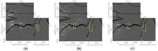
Figure 8.
Middle West-dipping Fault. Kinematics: P-wave Velocity Down & S-wave Velocity Up (P–S image) of (a) Wr = synthetic 4 fault model, (b) Wr = Field Brady’s field data (c) Wr = Pure Noise.
3.2.3. Far Eastern-Dipping Fault
Figure 9 is another flattened cube of the P–S results; the depth slice is almost 300 m deeper, the PoroTomoY slice is about 650 m East, and the PoroTomoX slice is almost 300 m North of Figure 8. The far Eastern-dipping fault is highlighted in the three yellow boxes. In the inline (PoroTomoY) slice there appears to be a bright spot in the eastern-dipping fault where the dip-angle is dramatically changing from steep to flat. The depth slice also shows potential for picking up the very top of the deepest of the three Western-dipping faults. This is encouraging considering it is at farthest distance from the receivers (DAS fiber), and quite deep at 580 m. The image created with Wr = Pure Noise (Figure 9c) further confirms that the signals in the yellow box on the inline slice is due to the changing dip of the Eastern dipping fault, and not artifacts.
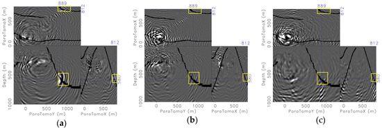
Figure 9.
Far Eastern dipping fault. Kinematics: P-wave Velocity Down & S-wave Velocity Up (P–S image) of (a) Wr = synthetic 4 fault model, (b) Wr = Field Brady’s field data (c) Wr = Pure Noise.
4. Discussion
Velocity uncertainty is one of the factors that reduces the ability of RTM to accurately image the location of the faults. The estimates of P-wave velocity versus depth around the location of Well 56-1A varies between different tomography methods [28,29] and the interval velocity obtained directly from the DAS data [26]. This, along with an imperfect fault model, that is based on legacy seismic and well information, will create uncertainty and variability within our images.
The effect of the velocity model can be seen in some of the RTM images. In the depth slice (upper left) of the a and b images in Figure 8, the focusing effect of the velocity model is seen along the middle West-dipping fault (see Figure 4 for the general patterns of the velocity). Focusing is caused by patterns of higher velocities, in this case, these may be artifacts of the acquisition geometry itself [28]. Focusing is also seen in the PoroTomoX and PoroTomoY panels. In the lower right panels, there are brighter spots that begin PoroTomoX = 500 and depth = 500, which coincide with a higher (4500 m/s versus 4000 m/s) velocity structure. There are also focusing patterns below the yellow box in the lower left panels.
Another modeling approach that could be considered is a Kirchhoff migration [30]. Kirchhoff is ray-based, and although it may not capture the mode-conversion and scattering of wave-equation-based methods, it could result in fewer migration artifacts, which are highly present, given the non-ideal geometry of the vibe points, and the fiber in Well 56-A1. A more thorough analysis of the wavefields used during the imaging process with RTM may provide some angles of reflection, thus insight into the mode conversions by confirming the angles of incidence for the shot sources and faults [31]. With angles of incidence, we may be able to explain where P to S mode conversions occur via Zoeppritz equations.
Future research directions should focus on further processing the DAS data to isolate events of interest. Before migrating, the field data was filtered to remove downgoing events via simple Fourier analysis. The field data would be less noisy with expert processing applied, such as statics corrections. The geophone data was not useful to this end, as it suffered from spatial aliasing (average spacing of 80 m), and the short maximum offset of 1500 m in the DAS horizontal array did not allow adequate recording of moveout (e.g., for identification of hyperbolas) [32]. Also, this paper only utilized the P-mode sources (when the vibroseis truck “shook” up and down). Both shear-vertical (SV) and shear-horizontal (SH) sources were induced at every vibe point. Utilizing these multi-component sources would surely increase the information and certainty of the fault locations, as they may provide reflected energy that has particle direction aligned with the vertical fiber.
Because of Well 56-1A’s relative position to all the vibe points, it is very difficult to resolve any faults in the PoroTomoY plane that are close to or west of well location (PoroTomoX < 125 m). The results could be an argument for compressive sensing to help design acquisition geometry, especially when dealing with a limited budget and the restrictions such as fumaroles and permitting, which PoroTomo was with the Emigrant Trail [11]. Compressive sensing exploits the fact that a small and carefully selected set of measurements of a compressible signal carries enough information for reconstruction and processing [33].
As mentioned in the Introduction, DAS is considered to have a much lower signal-to-noise ratio compared to seismic data recorded on geophones. One issue is the gauge length, which is a type of spatial averaging done in the interrogator [15], but another issue is also the coupling mechanism of the fiber to the subsurface. It is remarkable, but not unheard of, that the unattached, hanging DAS fiber is able to recover usable signal. Lindsey et al. [34] describe how a variety of earthquakes are detectable using fiber deployed in standard telecommunications conduits, which are imperfectly coupled to the subsurface. Frictional coupling can allow for the fiber to record signal that is related to the subsurface media [35].
5. Conclusions
DAS data can be successfully used to produce images of the faults at the Brady field. These images are created with an RTM approach to map P–P and P–S waves in the subsurface. Despite the many challenges in the DAS Brady data (reverberating fiber, multiple interfering events, location in extreme southern portion of vibe points, lack of resources for processing), structure of the faults were confirmed via comparisons with the synthetic data. Our analysis suggests that a denser vibe point coverage would produce cleaner migrated images by stacking out artifacts. However, we show that a careful modeling of synthetic data with the same source/receiver geometry and velocity models used in the field data experiment, can help us (1) isolate geometry or velocity effects and (2) attempt to distinguish migration artifacts from true geologic structures. These imaging results show the potential for DAS sensors to locate faults, which are the lifeblood of conventional geothermal fields.
Author Contributions
The authors contributed in the following categories: conceptualization, W.T.-G. and A.G.; methodology, A.G.; software, A.G.; validation, W.T.-G., A.G. and B.S.; formal analysis, W.T.-G.; investigation, W.T.-G.; resources, A.G.; data curation, W.T.-G., S.J., H.P.; writing—original draft preparation, W.T.-G.; writing—review and editing, W.T-G., A.G.; visualization, W.T.-G., B.S.; supervision, W.T.-G.; project administration, W.T.-G.; funding acquisition, W.T.-G.
Funding
This research was funded in part by the Office of Energy Efficiency and Renewable Energy (EERE), U.S. Department of Energy, under Award Numbers DE-EE0006760 and DE-EE0005510.
Acknowledgments
The authors thank the PoroTomo team for their support in this research.
Conflicts of Interest
The authors declare no conflict of interest.
References
- Mondol, N. Seismic Exploration. In Petroleum Geoscience: From Sedimentary Environments to Rock Physics; Springer Science & Business Media: Berlin/Heidelberg, Germany, 2010; p. 508. [Google Scholar]
- Sheriff, R.E.; Geldart, L.P. Exploration Seismology; Cambridge University Press: Cambridge, UK; New York, NY, USA, 1995. [Google Scholar]
- Allaby, M. (Ed.) A Dictionary of Geology and Earth Sciences; Oxford University Press: Oxford, UK, 2013. [Google Scholar]
- Gritto, R.; Daley, T.M.; Majer, E.L. Seismic Mapping of the Subsudace Structure at the Ryepatch Geothermal Reservoir; DOEEEGTP (USDOE Office of Energy Efficiency and Renewable Energy Geothermal Tech Pgm): Berkeley, CA, USA, 2000. [Google Scholar]
- Melosh, G.; Cumming, W.; Casteel, J.; Niggemann, K.; Fairbank, B. Seismic Reflection Data and Conceptual Models for Geothermal Development in Nevada. In Proceedings of the World Geothermal Congress 2010, Bali, Indonesia, 25–29 April 2010; pp. 25–29. [Google Scholar]
- Huang, L.; Gao, K.; Huang, Y.; Cladouhos, T.T. Anisotropic Seismic Imaging and Inversion for Subsurface Characterization at the Blue Mountain Geothermal Field in Nevada. In Proceedings of the 43rd Workshop on Geothermal Reservoir Engineering, Stanford, CA, USA, 12–14 February 2018; pp. 1–10. [Google Scholar]
- Folsom, M.; Lopeman, J.; Perkin, D.; Sophy, M. Imaging Shallow Outflow Alteration to Locate Productive Faults in Ormat’s Brady’s and Desert Peak Fields Using CSAMT. In Proceedings of the 43rd Workshop on Geothermal Reservoir Engineering, Stanford, CA, USA, 12–14 February 2018; pp. 1–11. [Google Scholar]
- Coolbaugh, M.F.; Sladek, C.; Kratt, C.; Edmondo, G. Digital mapping of structurally controlled geothermal features with GPS units and pocket computers. Geotherm. Resour. Counc. Trans. 2004, 28, 321–325. [Google Scholar]
- Faulds, J.E.; Coolbaugh, M.F.; Benoit, D.; Oppliger, G.; Perkins, M.; Moeck, I.; Drakos, P. Structural Controls of Geothermal Activity in the Northern Hot Springs Mountains, Western Nevada: The Tale of Three Geothermal Systems (Brady’s, Desert Peak, and Desert Queen). Geotherm. Resour. Counc. Trans. 2010, 34, 675–683. [Google Scholar]
- Siler, D.L.; Faulds, J.E. Three-Dimensional Geothermal Fairway Mapping: Examples from the Western Great Basin, USA. GRC Trans. 2013, 37, 327–332. [Google Scholar]
- Feigl, K.L.; Lancelle, C.; Lim, D.D.; Parker, L.; Reinisch, E.C.; Ali, S.T.; Fratta, D.; Thurber, C.H.; Wang, H.F.; Robertson, M.; et al. Overview and Preliminary Results from the PoroTomo project at Brady Hot Springs, Nevada: Poroelastic Tomography by Adjoint Inverse Modeling of Data from Seismology, Geodesy, and Hydrology. In Proceedings of the 42nd Workshop on Geothermal Reservoir Engineering, Stanford, CA, USA, 13–15 February 2017; pp. 1–15. [Google Scholar]
- Ali, S.T.; Akerley, J.; Baluyut, E.C.; Davatzes, N.C.; Lopeman, J.; Moore, J. Geodetic Measurements and Numerical Models of Deformation: Examples from Geothermal Fields in the Western United States. In Proceedings of the 41st Stanford Workshop on Geothermal Reservoir Engineering, Stanford, CA, USA, 22–24 February 2016. [Google Scholar]
- Queen, J.H.; Daley, T.M.; Majer, E.L.; Nihei, K.T.; Siler, D.L.; Faulds, J.E. Surface Reflection Seismic and Vertical Seismic Profile at Brady’s Hot Springs, NV, USA. In Proceedings of the 41st Stanford Workshop on Geothermal Reservoir Engineering, Stanford, CA, USA, 22–24 February 2016. [Google Scholar]
- Feigl, K.; Team, P. Overview and Preliminary Results from the PoroTomo project at Brady Hot Springs, Nevada: Poroelastic Tomography by Adjoint Inverse Modeling of Data from Seismology, Geodesy, and Hydrology. In Proceedings of the 43rd Workshop on Geothermal Reservoir Engineering, Stanford, CA, USA, 12–14 February 2018. [Google Scholar]
- Dean, T.; Cuny, T.; Hartog, A.H. The effect of gauge length on axially incident P-waves measured using fibre optic distributed vibration sensing. Geophys. Prospect. 2017, 65, 184–193. [Google Scholar] [CrossRef]
- Hornman, J.C. Field trial of seismic recording using distributed acoustic sensing with broadside sensitive fibre-optic cables. Geophys. Prospect. 2017, 65, 35–46. [Google Scholar] [CrossRef]
- Lumens, P.G.E. Fibre-Optic Sensing for Application in Oil and Gas Wells. Ph.D. Thesis, Eindhoven University of Technology, Eindhoven, The Netherlands, 2014. [Google Scholar]
- Mateeva, A.; Lopez, J.; Potters, H.; Mestayer, J.; Cox, B.; Kiyashchenko, D.; Wills, P.; Grandi, S.; Hornman, K.; Kuvshinov, B.; et al. Distributed acoustic sensing for reservoir monitoring with vertical seismic profiling. Geophys. Prospect. 2014, 62, 679–692. [Google Scholar] [CrossRef]
- Daley, T.M.; Miller, D.E.; Dodds, K.; Cook, P.; Freifeld, B.M. Field testing of modular borehole monitoring with simultaneous distributed acoustic sensing and geophone vertical seismic profiles at Citronelle, Alabama. Geophys. Prospect. 2016, 64, 1318–1334. [Google Scholar] [CrossRef]
- Raterman, K.T.; Farrell, H.E.; Mora, O.S.; Janssen, A.L.; Gomez, G.A.; Busetti, S.; Mcewen, J.; Davidson, M.; Friehauf, K.; Rutherford, J.; et al. Sampling a Stimulated Rock Volume: An Eagle Ford Example. In Proceedings of the Unconventional Resources Technology Conference, Austin, TX, USA, 24–26 July 2017; pp. 24–26. [Google Scholar]
- Michlmayr, G.; Chalari, A.; Clarke, A.; Or, D. Fiber-optic high-resolution acoustic emission (AE) monitoring of slope failure. Landslides 2017, 14, 1139–1146. [Google Scholar] [CrossRef]
- Daley, T.; Freifeld, B.; Ajo-Franklin, J.; Dou, S.; Shulakova, V.; Kashikar, S.; Miller, D.E.; Goetz, J. Field testing of fiber-optic distribued acoustic sensing (DAS) for subsurface seismic monitoring. Lead. Edge 2013, 32, 699–706. [Google Scholar] [CrossRef]
- Claerbout, J. Toward a unified theory of reflector mapping. Geophysics 1971, 36, 467–481. [Google Scholar] [CrossRef]
- Yang, T.; Shragge, J.; Sava, P. Illumination compensation for image-domain wavefield tomography. Geophysics 2013, 78, U65–U76. [Google Scholar] [CrossRef][Green Version]
- Claerbout, J. Introduction to Seplib and SEP utility software. Stanf. Explor. Proj. 1991, 413, 436. [Google Scholar]
- Miller, D.E.; Coleman, T. DAS and DTS at BradyHot Springs: Observations about Coupling and Coupled Interpretations. In Proceedings of the 43rd Workshop on Geothermal Reservoir Engineering, Stanford, CA, USA, 12–14 February 2018. [Google Scholar]
- Woodward, M.J. Wave-equation tomography. Geophysics 1992, 57, 15–26. [Google Scholar] [CrossRef]
- Matzel, E.; Zeng, X.; Thurber, C.; Luo, Y.; Morency, C. Seismic Interferometry Using the Dense Array at the Brady Geothermal Field. In Proceedings of the 42nd Workshop on Geothermal Reservoir Engineering, Stanford, CA, USA, 13–15 February 2017; pp. 3–6. [Google Scholar]
- Thurber, C.; Zeng, X.; Parker, L.; Lord, N.; Fratta, D.; Wang, H.; Matzel, E.M.; Robertson, M.; Feigl, K.L.; PoroTomo Team. Active-Source Seismic Tomography at Bradys Geothermal Field, Nevada, with Dense Nodal and Fiber-Optic Seismic Arrays. Seismol. Res. Lett. 2018, 89, 1629–1640. [Google Scholar]
- Hokstad, K. Multicomponent Kirchhoff migration. Geophysics 2002, 65, 861–873. [Google Scholar] [CrossRef]
- Rickett, J.; Sava, P.C. Offset and angle-domain common image-point gathers for shot-profile migration. Geophysics 2002, 67, 883–889. [Google Scholar] [CrossRef]
- Jreij, S.; Trainor-Guitton, W.; Simmons, J. Improving Point-Sensor Image Resolution with Distributed Acoustic Sensing at Brady’s Enhanced Geothermal System. In Proceedings of the 43rd Workshop on Geothermal Reservoir Engineering, Stanford, CA, USA, 12–14 February 2018. [Google Scholar]
- Allegar, N.; Herrmann, F.J.; Mosher, C.C. Introduction to this special section: Impact of compressive sensing on seismic data acquisition and processing. Lead. Edge 2017, 36, 622–708. [Google Scholar] [CrossRef]
- Lindsey, N.J.; Martin, E.R.; Dreger, D.S.; Freifeld, B.; Cole, S.; James, S.R.; Biondi, B.L.; Ajo-Franklin, J.B. Fiber-Optic Network Observations of Earthquake Wavefields. Geophys. Res. Lett. 2017, 44, 11792–11799. [Google Scholar] [CrossRef]
- Munn, J.D.; Coleman, T.I.; Parker, B.L.; Mondanos, M.J.; Chalari, A. Novel cable coupling technique for improved shallow distributed acoustic sensor VSPs. J. Appl. Geophys. 2017, 138, 72–79. [Google Scholar] [CrossRef]
© 2019 by the authors. Licensee MDPI, Basel, Switzerland. This article is an open access article distributed under the terms and conditions of the Creative Commons Attribution (CC BY) license (http://creativecommons.org/licenses/by/4.0/).