1. Introduction
Geothermal energy is a renewable energy resource for low carbon heat and power production. The techno-ecological potential for geothermal electricity production in Germany is estimated by the German Federal Environment Agency to be up to 8.5 GW or 63.75 TWh/a [
1]. For the conversion of the thermal energy of brine to electrical energy, usually the organic Rankine cycle (ORC) is used. An additional heat supply can improve the flexibility of these power plants. Since thermal water is needed for the heat generation, the electrical power output is reduced. Due to the different remuneration of heat and power, there are also economic effects. However, previous investigations have shown that additional heat extraction increases the efficiency and the profitability of geothermal power plants [
2,
3]. Due to the fluctuating heat demand, the ORC plant is driven more often in part load conditions. To analyze systems operating in part load, quasi-stationary or transient simulation models are used. In literature, dynamic models of ORC are mainly developed for waste heat recovery applications in vehicles and diesel engines. Huster et al. [
4] present a dynamic model of a basic ORC for waste heat recovery in a diesel truck. For modelling, the commercial software gPROMS is used and the model is validated by a transient measurement data set. The study shows that the initialization process is a challenging task and the dynamics in the heat exchangers are mostly dominated by the pressure level. Galindo et al. [
5] use a dynamic ORC model to investigate heat recovery by transportation vehicles. The results show that the maximum power delivered by the ORC is 800 W and the fuel conversion efficiency can be increased by 2.5%. Jiaxin Ni et al. [
6] developed a dynamic ORC model in Dymola/Modelica for waste heat recovery from diesel engines. They investigated the direct heat recovery by an ORC and the integration of an intermediate oil cycle. The results show that the thermal inertia of the oil cycle damps the system. Bin Xu [
7] also consider diesel engines as a heat source. They developed a dynamic model of a one stage ORC with parallel evaporators in MATLAB/Simulink and validated the model against experimental results. The vapor temperature and the evaporation pressure can be predicted within 2% and 3% mean error. Baccioli et al. [
8] investigated a solar ORC with compound parabolic collectors. Therefore, a dynamic model of an ORC with a recuperator was developed. The results show that there is a control strategy, which is able to drive the plant without the need of a thermal storage. Proctor et al. [
9] developed a dynamic ORC model for a geothermal power plant. The model is validated by a standard deviation of 1.4%. So far, only small-scale or one-stage transient simulations are conducted. Double-stage geothermal ORC are not considered yet.
Concerning combined heat and power (CHP) generation by ORC generally, Wieland et al. [
10] investigated several CHP plant concepts for the ORC. As a heat source, the exhaust gas of an internal combustion engine is considered. The exhaust gas temperature is assumed to be 490 °C. They considered the serial, parallel, serial/parallel configuration and different concepts with the district heating system fed by the cooling water of the ORC. Moreover, the authors investigate a concept with turbine bleeding. In this concept, the working fluid is split between the two turbine stages to serve the heat demand. The simulations are perfomed by steady state simulations including the part load behavior of the heat exchangers. The heat demand is estimated by an annual load duration curve and different working fluids are investigated. The results show that the turbine bleeding concept can produce at least 12% more electrical power than the other concepts. Van Erdeweghe et al. [
11,
12,
13] considered different CHP plant concepts fed by a low enthalpy geothermal source. Their research focused on a steady state model of a one-stage ORC with and without a recuperator. At first, the serial and parallel CHP concept is compared to pure electricity production [
11]. The results show the serial concept is suitable to low temperature district heating networks. The parallel configuration allows delivering of high temperature district heating networks. For all considered CHP concepts, plant efficiency is higher than for the reference case, the pure electricity production. In [
12] a so called “preheat-parallel” concept is introduced. In this configuration, the thermal water exiting the ORC is used to preheat the district heating network fluid. Additionally, mass flow rate is coupled to the district heating system before entering the ORC (parallel configuration) to reach the supply temperature. The preheat-parallel concept leads to a 5.3% higher net electrical power output and to the highest exergetic plant efficiency of 38.3%. Van Erdeweghe et al. [
13] extended this study by including the HB4 configuration, where the brine is split and fed to the district heating system at the evaporator outlet.
To sum up, the previous work on CHP-ORC plants is based on steady state ORC models and the part load behavior is partially considered by quasi-stationary simulations. The heat demand is modelled by an annual load duration curve or assumed to be constant. The evaluation of the CHP concepts is based on thermodynamic parameters. In this study, a dynamic model of an ORC is developed to cover the fluctuating heat demand and ambient temperature during the day. Instead of a one-stage ORC, a double-stage ORC is considered. The heat demand profiles are developed based on a real geothermal district heating network. Different CHP concepts are investigated and compared to the pure electricity production (reference case). Annual simulations are performed for a resilient evaluation of different CHP concepts based on thermodynamic and economic parameters.
In
Section 2 the dynamic simulation model is described. Moreover, a method for performing annual dynamic simulations and the development of corresponding heat demand profiles is introduced.
Section 3 consists of the model validation and the results for the considered CHP concepts compared to the reference case.
2. Methods
The evaluation of geothermal CHP plant concepts is based on annual simulations inspired by the method according to VDI 4655 [
14]. Therefore, a dynamic simulation model and heat demand profiles are required.
2.1. Annual Simulations Based on VDI 4655
In the VDI 4655 [
14] typical days of the year are defined. Next to the season, summer (S), winter (W) and transition (Ü) the typical days are differentiated between workdays (W) and Sundays (S) to account for the different user behavior. In this context, Saturdays are assigned to the workday category. In addition, fine (H) and cloudy (B) days are distinguished. However, for the summer days the differentiation between cloudy and fine is negligible (X). Based on these criteria 10 typical days can be defined (
Table 1). [
14]
Germany is divided in different climate zones with corresponding test reference years (TRY).
Table 2 shows an excerpt of the TRY for the climate zones 12 to 14. Depending on the climate zone, the frequency of typical days per category for one year (
n) varies. For example, in TRY12 there are 57 cloudy winter workdays in one year and in TRY13 there are 91 [
14]. For an annual simulation, the 10 typical days are simulated for TRY13, which refers to the southern German Molasse Basin. An annual simulation is obtained by weighting these typical days according to their frequency
n (see
Table 2).
2.2. Heat Demand Profiles
Next to a dynamic simulation model, heat demand profiles for each typical-day category are needed to perform annual simulations.
The corresponding heat demand profiles are developed based on operational data of a real geothermal heat plant in the German Molasse Basin. The applied method is based on the VDI-report reference load profiles [
15] and adapted for the analysis of real operational data. Furthermore, the method is extended for a systematic identification of outlying load profiles and, for weather adjustment, the degree days method of VDI 3807 [
16] is implemented.
In the first step, the raw operational data for one year of a real geothermal district heating network is analyzed and incomplete or incorrect data points are excluded. Next, the days are allocated to the typical day categories according to VDI 4655 [
14]. In this context, available weather data of 2016 is analyzed. The ambient temperature was measured in the heat plant and the cloud coverage was taken from the nearest weather station of the German Weather Service (DWD) [
17]. In a further step, the load profiles of each typical day category are standardized and outliers are identified by a box-whisker-plot [
18]. Then the squared error for each load profile from the mean values is calculated. As a result, the load profile with the lowest squared error becomes the reference load profile (RLP) for the typical day category.
The actual heat demand strongly depends on the weather conditions. Therefore, the RLPs are adjusted for the weather conditions based on the degree day method by VDI 3807. Based on this method RLPs for the 10 typical-day categories are developed.
Next to heat demand profiles, corresponding ambient temperature characteristics are needed as an input for the annual CHP simulations. By the method shown above, the heat demand profile of the day with the lowest squared error from the mean value becomes the RLP. Therefore, this day is the most characteristic for the corresponding typical day category. For this reason, the ambient temperature of this day is used as an input for the annual simulations.
2.3. Dynamic Simulation Model
The dynamic ORC simulation model is built up in Dymola [
19] based on the ThermoCycle [
20] library. For the calculation of fluid properties, the software Coolprop [
21] is used.
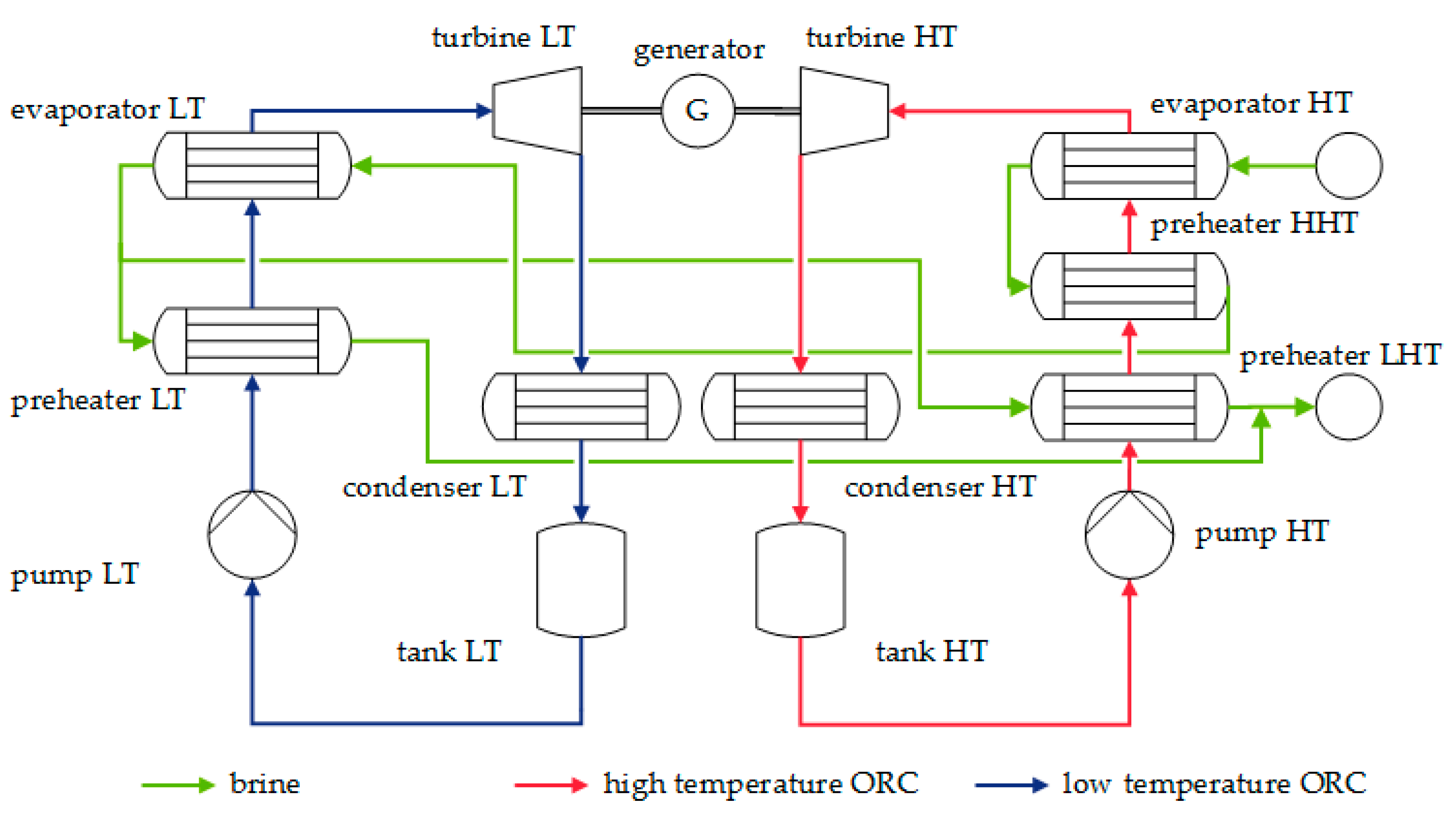
A double-stage ORC is modelled based on an existing geothermal power plant in the German Molasse Basin (
Figure 1). This is the basis for all investigations in this study.
The double stage ORC consists of a low-temperature (LT) and a high-temperature (HT) unit. The working fluid in both ORC modules is R245fa. Both units contain a pump, several preheaters, an evaporator, a turbine and a condenser. Firstly, the brine feeds the HT-evaporator and the HHT-preheater before the LT-evaporator is entered. At the outlet of the LT-evaporator the brine mass flow rate is split to the LT- and LHT-preheater before it is reinjected. The design parameters and some characteristic data for the rotating equipment and the heat exchangers are summarized in
Table 3. A corresponding
T-
-diagram is shown in
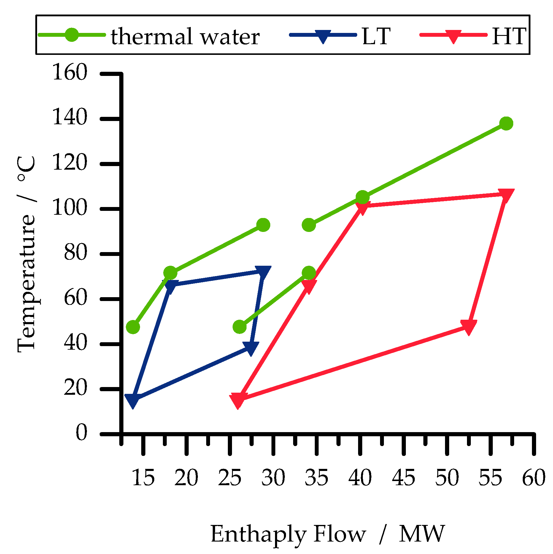
Figure 2.
From the power plant scheme, it is clear that in principle two types of components have to be modelled in Dymola: turbomachines (pumps and turbines) and heat exchangers (preheaters, evaporators and condensers). Since the time constants of expansion and compression machines are relatively small compared to those of the heat exchangers, the pumps and turbines can be modelled as quasi-stationary models [
22,
23,
24]. Therefore, for the pump a characteristic curve for the efficiency depending on the pumped volume flow rate from the datasheet of the manufacturer is implemented. The exhaust enthalpy is calculated according to:
h is the specific enthalpy,
ρ the density,
p the pressure of the working fluid and
ηs the isentropic efficiency of the pump. The indices indicate the inlet and outlet conditions. For the expansion, a turbine model is used based on Stodola’s law:
is the mass flow rate of the working fluid. The coefficient
K is calculated for the HT- and the LT-ORC by the respective nominal turbine inlet and outlet conditions. The isentropic efficiencies at the design point are given in
Table 3. The isentropic efficiency of the turbine in off-design is calculated by the correlation of Ghasemi et al. [
25].
For the heat exchangers, dynamic models are built up in three steps. At first, a stationary model with appropriate correlations for the heat transfer coefficient is developed. In the next step, the heat transfer coefficient
αnom for the design case is calculated. Afterwards, the correlations are simplified and a dynamic heat transfer coefficient is calculated based on the design case [
22].
The preheaters are shell and tube heat exchangers with double segmental baffles and two passes. They are implemented as finite-volume models. For each volume the dynamic energy balance is solved:
Vi is the volume of the cell, ρi the density and the supplied thermal power. h is the specific enthalpy, p the pressure and the mass flow rate. The subscripts indicate the inlet and outlet of the cell.
For the shell side heat transfer coefficient and pressure drop calculation, an adapted version of the Bell-Delaware method according to Milcheva et al. [
26] is used. For all considered heat exchangers, the tube side heat transfer coefficient is calculated according to Gnielinski [
27] and the pressure drop according to Kast and Nirschl [
28].
The evaporators are designed as kettle boilers with four passes on the tube side. According to Pili et al. [
29], the evaporators are implemented as two-volume models. It is a combination of the moving boundary and the finite-volume approach. For the brine on the tube side, the finite-volume approach is used. The shell side flow is divided in a vaporizing liquid and vapor volume. The natural convection heat transfer coefficient is set to 250 W/m²K [
30]. The pool boiling heat transfer coefficient is calculated by Mostinski [
31]. For the film boiling the Bromley equation is used [
32]. The bundle effect is taken into account according to Taborek [
33]. Regarding the pressure drop in kettle boilers, the static pressure drop due to the liquid level is considered [
34].
The condensation of the working fluid takes place in air-cooled finned tube bundles with two passes. The finite volume approach is used to model the condensers. The condensation heat transfer coefficient is calculated according to Cavallini et al. [
35]. For the two-phase pressure drop the correlation of Friedel [
36] is used. The airside heat transfer coefficient is calculated by the Haaf correlation [
37].
2.4. Combined Heat and Power (CHP) Plant Concepts
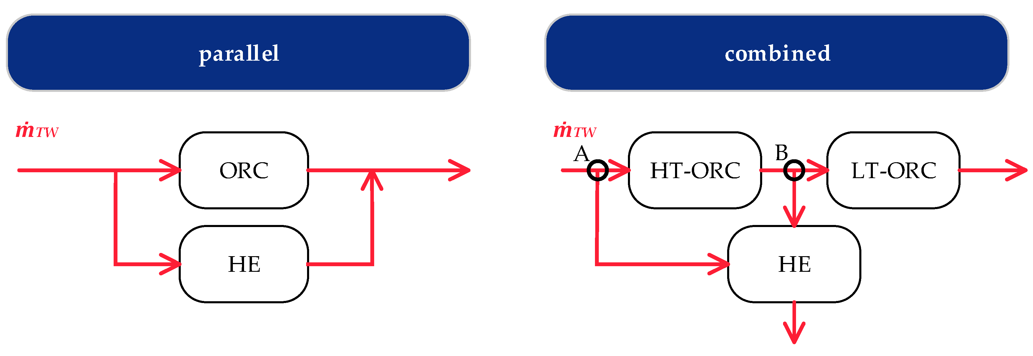
In this study, three geothermal CHP concepts are considered: the parallel, the parallel-HHT and the combined heat extraction (
Figure 3).
The operational strategy for the CHP plants is heat-driven; this means the head demand must be satisfied at any time of the day. For the parallel heat extraction, the thermal water is split before entering the HT-ORC evaporator and for the parallel-HHT configuration the thermal water is split after the HT-ORC evaporator and before the HHT preheater. For the combined concept, the thermal water is split before entering the HT-ORC (point A) and, in addition, heat is extracted between the LT- and the HT-ORC unit (point B). It should be noted that for the ORC-power system for all CHP-configurations the same existing ORC-module is considered.
Concerning the district heating network (DHN), a peak load of 5 MW is considered with a supply temperature of 90 °C and return temperature of 60 °C. The thermal energy delivered is 21.5 GWh per year. For the heat extraction (HE), a plate heat exchanger is assumed according to the data sheet of the real heat plant considered. The heat exchange area is 176.6 m². For the calculation of the heat transfer coefficient the Martin approach [
38] is used.
2.5. Thermodynamic and Economic Evaluation Parametes
The different CHP-concepts are evaluated by thermodynamic and economic parameters. The concepts are compared to the reference case, the pure electrical power generation.
For the thermodynamic evaluation, the second law net efficiency is used:
The exergy flow is calculated by:
The net power Pel,net is defined as the difference between the electrical power generated Pel,gross and the power consumption of the cycle. The power consumption of the cycle is composed of the power required for the pump Pel,pump as well as for the fans Pel,fans of the air-cooled condensers and the auxiliary components Pel,aux. For the auxiliary components and the power required for the fans of the condensers, the power consumption is estimated according to operational data by 788.36 kW. is the exergy flow rate of the heat source (HS) and to the district heating network (DHN). The dead state (Index 0) is assumed to be at 15 °C and 1 bar.
For the economic evaluation, the annual profit is calculated. For the electrical power the price
pel for 1 kWh is fixed by § 45 of the Erneuerbare–Energien–Gesetz to 25.2 c€ [
39]. For the thermal power delivered (
the mean price
pHE for district heating in Germany in 2017 (106.1 € per MWh [
40]) is assumed. The annual profit is calculated by Equation (4):
Due to the fact that for all considered configurations the same power plant is used, the investment costs for the power plant can be neglected as they are equal for all concepts. In a first step, the evaluation is based only on the revenues. In future work, a detailed economic model is developed to account for different district heating networks in terms of temperature level and peak load.
3. Results
At first, the dynamic simulation model is validated. Afterwards, the developed heat demand profiles are presented. Then, the results for the different CHP-concepts are shown and evaluated by the exergetic efficiency and the annual profit. The CHP-concepts are compared to the reference case, pure electricity production.
3.1. Evaluation of the Dynamic Behavior
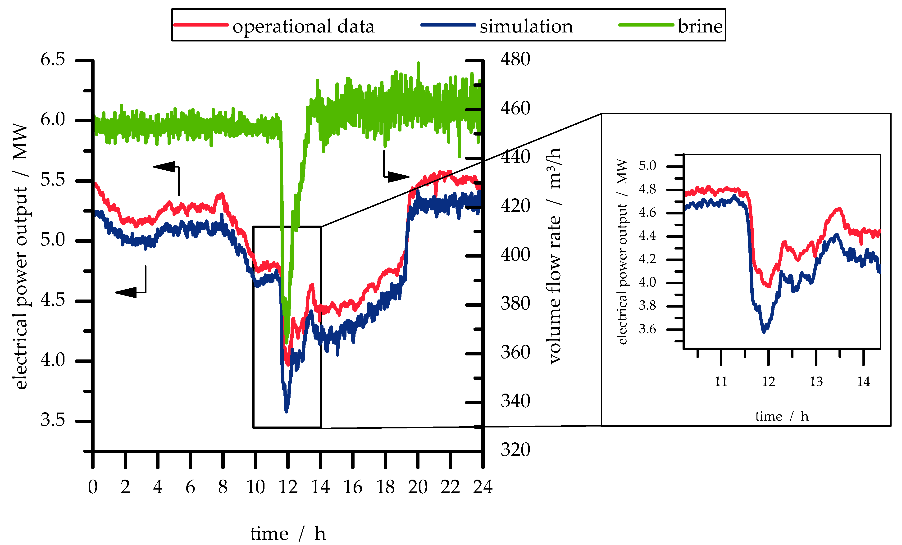
To validate the double-stage ORC, a period of 24 hours is simulated in steps of one minute. For the investigation of CHP-concepts the electrical power output is important and, therefore, this parameter is validated. The simulation results are compared to real operational data with a step in the brine volume flow rate. The step in the flow rate could represent a sudden change in the heat demand (
Figure 4). The results are shown in
Figure 4.
Obviously, the simulation model matches the dynamics of the real power plant. The relative root mean squared error (RRMSE) is 3.9%. For the detailed evaluation of the dynamic behavior, the Pearson correlation coefficient is used according to Sarin et al. [
41]. A correlation coefficient of +1 shows that there is a perfect linear relationship between the two time histories and they are identical in shape [
41]. The correlation coefficient between the simulated and measured electrical power output is 0.99 and shows that the simulation model can represent the dynamic behavior of the double-stage ORC. The validation results for further thermodynamic parameters are shown in
Table 4. The RRMSE is lower than 5% except for the volume flow rate of the HT-ORC. According to the manufacturer, the uncertainties of the integrated flow rate sensors are responsible for the deviations of the volume flow rates. A detailed description and validation of the simulation model is shown in [
42].
As an input for the simulation, the measured volume flow rate of the thermal water in the real power plant is used. In general, this measurement device is related to high uncertainties. For that reason, the simulated electrical power output is lower than the measured one even though no heat losses to the ambient are considered. Geothermal reservoirs usually provide a fixed volume flow rate. For the simulations, the volume flow rate is defined directly in the model and, therefore, the results are not affected by measurement uncertainties.
The validation of the model shows that even volatile changes of the brine mass flow rate can be simulated. The shown step of the brine mass flow rate (
Figure 4) leads to a gradient in electrical power of 1.3 kW/s. Therefore, the dynamic model even offers the possibility to investigate the capacity of the power plant to provide balancing power.
In this study, different concepts for geothermal heat and power production are evaluated by annual simulations. A widely used approach for conducting annual simulations is based on quasi-stationary models by assuming a mean ambient temperature. In contrast, the fluctuating ambient temperature over the day is considered by dynamic models. A comparison of these two methods shows a mean deviation of the exergetic efficiency of 3.3%. In particular, for the winter days the mean ambient temperature assumption leads to at least 4% higher exergetic efficiencies in case of the quasi-stationary model. For example, for the typical day category WWB the exergetic efficiency is 7.9% higher. In terms of economic considerations, the annual return based on a mean ambient temperature is 160,000 € higher. Due to the deviations, for a resilient energetic and economic evaluation of different concepts for geothermal heat and power generation the developed dynamic model is used for further investigation.
3.2. Heat Demand Profiles
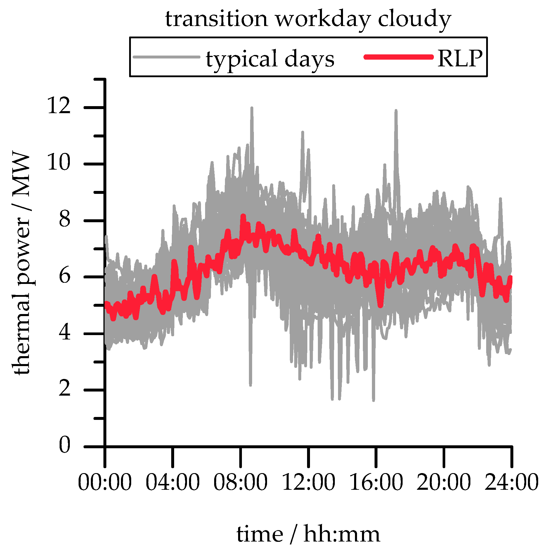
The RLP for all typical day categories are developed by the method shown in
Section 2.2. Exemplarily, the results are shown for the typical day ÜWB.
Figure 5 shows all heat demand profiles of this category (grey color) and the identified RLP (red color).
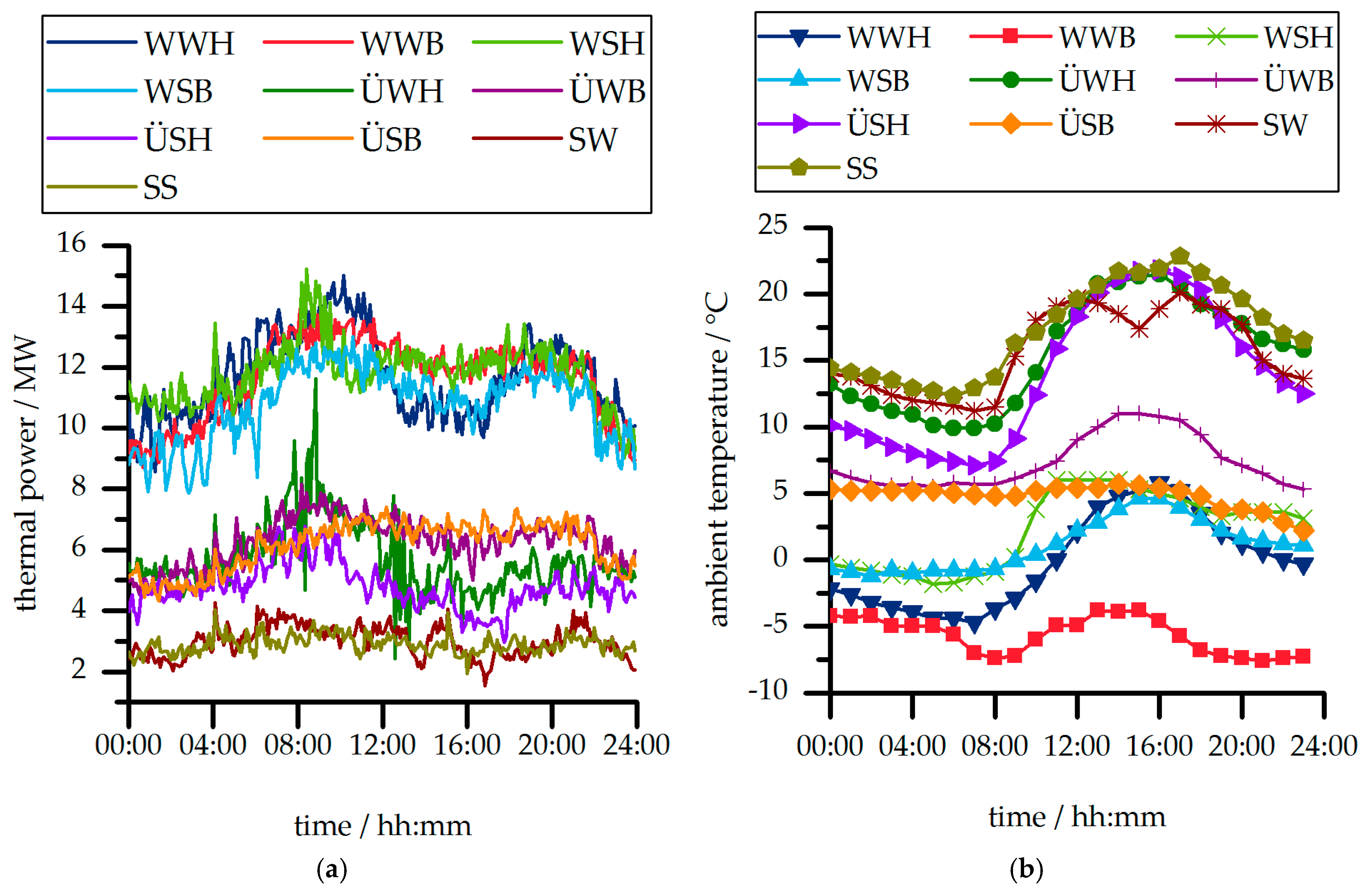
In the considered year, 45 days could be allocated to the category ÜWB. The figure shows that, based on the presented method, qualitatively and quantitatively characteristic heat demand profiles can be developed for each typical day category. All developed RLP and the corresponding ambient temperatures are shown in
Figure 6.
Regarding the RLP, each season of the year can be recognized by the heat demand. For the winter the heat demand is higher than for the transition days and for the summer days. In terms of the cloud coverage, it can be recognized that for fine days the heat demand in the afternoon is significantly lower than for cloudy days. In addition, the RLP show that for Sundays the heat demand is typically lower and shows smaller fluctuations than for workdays.
For the ambient temperature profiles, the lowest ambient temperatures occur in the winter followed by the transition and summer days. For fine and cloudy days, it can be recognized that the ambient temperature for fine days is in principle higher than for cloudy days.
3.3. Parallel Heat Extraction
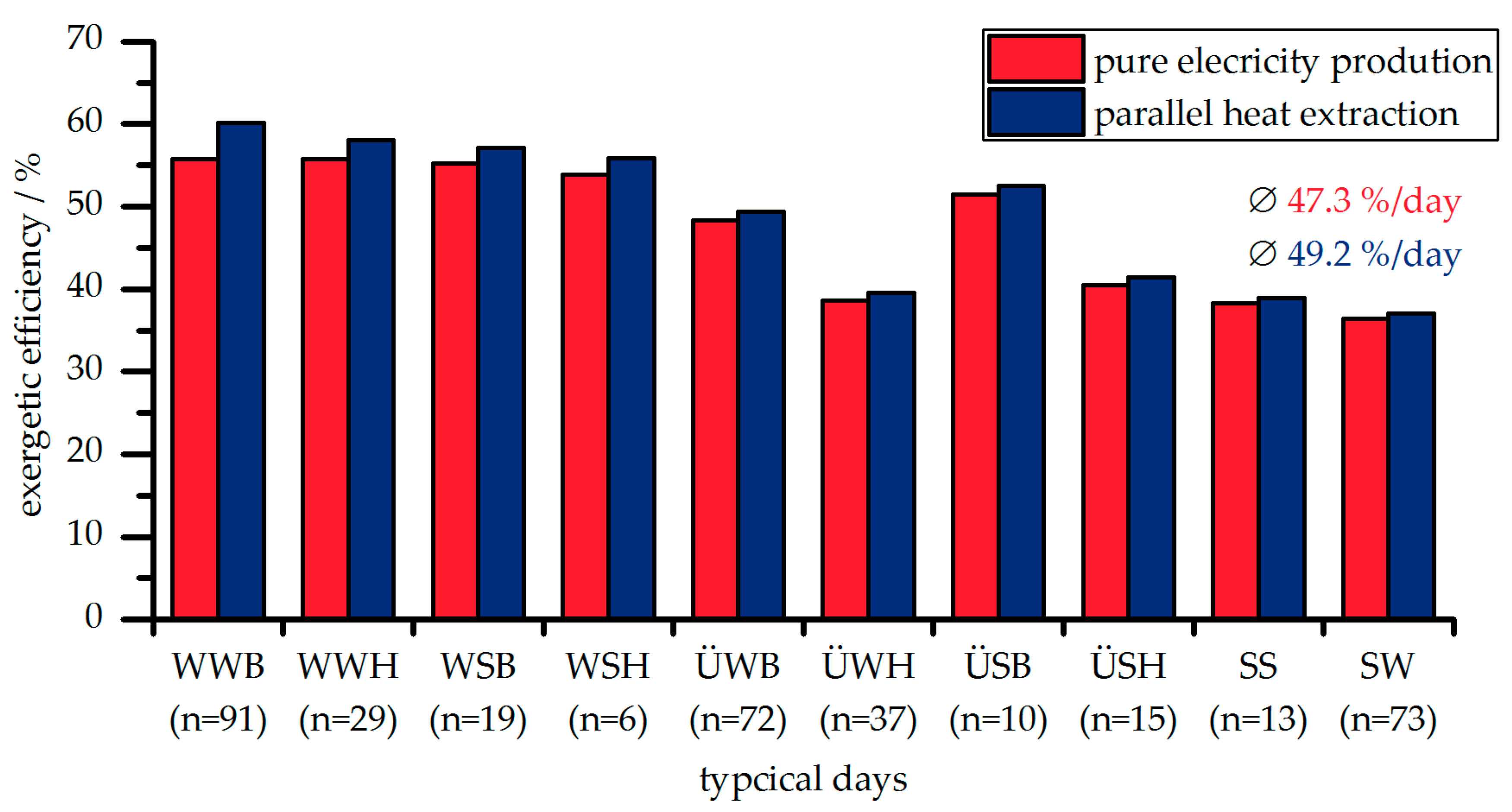
Figure 7 shows the mean exergetic efficiency of each typical day for pure electricity production and parallel heat extraction.
In general, the parallel heat extraction shows a higher exergetic efficiency than the pure electricity production for each typical day. For parallel heat extraction, the brine is split before entering the ORC to satisfy the heat demand. Therefore, the mass flow rate of thermal water fed to the ORC is lower than for pure electricity production and the amount of electrical power produced decreases. However, the additional heat delivered to the DHN compensates the decrease in electrical power production.
For the winter days, the heat demand is higher than for transition and summer days. Therefore, the increase in efficiency is higher for winter days. The highest increase occurs at WWB. The parallel concept shows a 7.9% higher exergetic efficiency than the pure electricity production. In this case, the produced electrical energy by the parallel concept is 6.1 MWh lower than for pure electricity production. However, the amount of additional heat extracted by the parallel concept is 91.9 MWh and overcompensates for the loss in electrical power production.
By multiplying the amount of electrical and thermal energy produced, respectively, with the assumed prices per kWh, the revenues for each typical day can be calculated. For an annual profit analysis, the results are scaled up by the frequency of the typical days in one year according to
Table 2.
Table 5 summarizes the revenues for the typical days for pure electricity production and parallel heat extraction.
In principle, the revenues per typical day can be increased by the parallel concept. The increase in profit is higher for the winter days than for the transition and summer days. The revenues can be increased by parallel heat extraction by up to 23.9%. The annual profit for the pure electricity production is calculated to 10.75 M€. It can be increased by parallel heat extraction by 16.1% to 12.48 M€.
3.4. Parallel-HHT Configuration
For the parallel-HHT heat extraction concept, the mass flow rate of the brine is split at the outlet of the evaporator of the HT-ORC and before entering the HHT-preheater. The exergetic efficiency is compared to the parallel concept in
Table 6.
The parallel-HHT concept shows slightly higher exergetic efficiencies (about 1.1%) than the parallel concept. The reason for that is the higher electrical power output of the parallel-HHT concept. Considering the LT- and the HT-module, the power output for the LT-module is lower for the parallel-HHT concept compared to the parallel concept. This effect is compensated by the higher power output of the HT-module.
Because of the heat extraction at the HT-evaporator outlet, there is lower thermal power available for preheating the working fluid in the HT-cycle. Therefore, higher thermal power is consumed in the HT-evaporator to vaporize the working fluid. Due to the heat extraction, a lower temperature level of the brine is fed to the LT-cycle, which leads to a lower power output. Nevertheless, in sum this lower power output is overcompensated by the higher power output of the HT-module.
For the typical day WSH, the highest increase of about 2.1% occurs. The electrical power output is 123.5 MWh and 3 MWh higher than for the parallel concept. In sum, the parallel-HHT concept produces 400 MWh more electrical energy than the parallel concept.
3.5. Combined Heat Extraction
For the combined heat extraction, concept the following operational strategy is considered: A certain amount of brine mass flow rate is coupled to the DHN between the HT-ORC and the LT-ORC (see
Figure 3 point B). Since the temperature of the brine between the two ORC-stages is lower than the supply temperature for the DHN (90 °C), the remaining brine mass flow rate to meet the supply temperature of the DHN is coupled to the DHN at the inlet of the HT-ORC (see
Figure 3 point A).
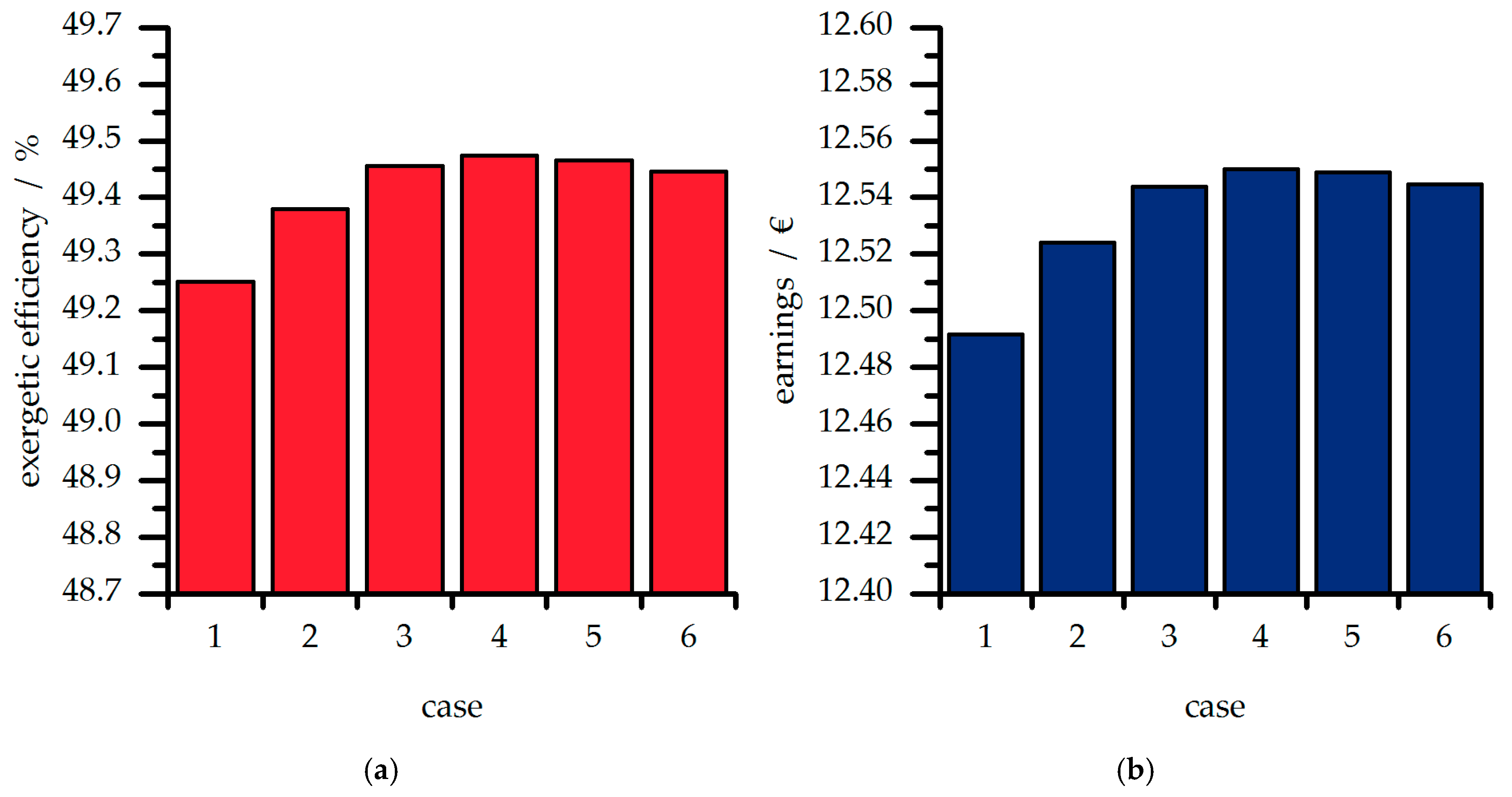
At first, the amount of the mass flow rate coupled to the DHN at point B in
Figure 3 is varied in steps of 5% to optimize the system performance in terms of efficiency. Overall, 6 cases are considered, where in case 1, 5% of the mass flow rate are fed to the DHN and in case 6, 30%, respectively. The results are shown in
Figure 8.
The annual mean exergetic efficiency increases up to case 4 and then decreases. With an increasing fraction of brine mass flow rate coupled to the DHN between LT-and HT-ORC a higher mass flow rate is fed to the HT-ORC module. This makes the HT-module produce more electrical energy. By further increasing of the mass flow rate coupled to the DHN between the ORC-modules, the thermal energy fed to the LT-cycle decreases and thus so does the electrical power produced by the LT-cycle. Compared to case 1, case 4 produces 232.8 MWh more electrical energy per year and case 6, 212.1 MWh.
The economic investigation shows that the annual revenues increase with the fraction of mass flow rate coupled to the DHN. From case 1 to case 4 the annual profit increases by about 58,000 €. Therefore, case 4 can be identified as optimal in terms of thermodynamic and economic considerations.
Case 4 (20% of the mass flow rate is coupled to the DHN) as the optimal combined heat extraction concept is now compared to the parallel heat extraction.
Table 7 shows the exergetic efficiency of each typical day for both heat extraction concepts.
In general, the combined concept shows a slightly higher exergetic efficiency (about 0.8%) than the parallel concept. For typical days WSH and ÜWH, the maximum increase of 1.3% occurs. Compared to the parallel concept, for the combined heat extraction a higher mass flow rate of the thermal water is fed to the HT-ORC, which leads to a slightly higher electrical power production. By the combined concept, 300 MWh more electrical energy can be produced per year.
The annual revenues are listed in
Table 8. Due to the slightly higher exergetic efficiency of the combined concept, also the revenues for the typical days are slightly higher than for the parallel concept. The maximum increase of the revenues is 1.2%. Analogous to the efficiency considerations, the revenues for the winter and transition days are higher than for the summer days. In total, the combined concept leads to about 76,000 € higher revenues per year than the parallel concept.
To sum up, for the considered DHN the combined heat extraction concept shows a slightly better exergetic efficiency than the parallel concept and leads to higher revenues per year.
4. Conclusions
In this study, a dynamic model of a double-stage organic Rankine cycle (ORC) is developed and validated by operational data of a real geothermal power plant in the southern German Molasse Basin. By the dynamic model, different heat extraction concepts for geothermal power plants are investigated. For the heat extraction, two parallel concepts and the combined concept are considered. The concepts are evaluated by the exergetic efficiency and the annual return. The reference case for the evaluation is the pure electricity production.
The parallel heat extraction concept shows higher exergetic efficiencies than the pure electricity production. The exergetic efficiency is on average 4.1% higher. Compared to the pure electricity concept, the electrical energy produced by the parallel concept decreases by 2.2 GWh/a. However, 21.5 GWh/a thermal power can be extracted to the DHN.
By extracting the heat after the HT-evaporator (parallel HHT-concept), the exergetic efficiency of the power plant can be increased by 1.1% and 400 MWh more electricity can be produced compared to the parallel concept. This leads to about 100,000 € higher annual returns than for the parallel concept.
For the combined concept, it is shown that the exergetic efficiency varies with the amount of mass flow rate extracted between the ORC modules. Based on the results, case 4 (20%) is the optimum. In comparison to the reference case, the pure electricity production, the combined concept shows a 4.6% higher exergetic efficiency. Regarding the economic evaluation, the annual return can be increased by 16.8%. Compared to the parallel concept, the combined concept leads to on average 0.8% higher exergetic efficiencies. Considering the electricity production, 300 MWh more electrical energy can be produced by the combined concept. In terms of the economic evaluation, the annual return can be increased through the combined concept by about 76,000 €.
To summarize, the efficiency and the profitability of geothermal power plants can be increased by additional heat extraction. The average thermal power of the geothermal fed district heating systems is 12.5 MW. Even for the relatively small considered district heating network with a peak load of 5 MW, the effects of an additional heat supply are clearly evident. The combined concept shows a slightly higher exergetic efficiency and annual return than the parallel concept. The parallel-HHT concept leads to even higher exergetic efficiencies than the combined concept and the annual return can be increased by up to 27% compared to the combined concept. In addition, the combined concept is more complex in terms of control equipment and strategies than the parallel-HHT concept and, therefore, the parallel-HHT should be preferred for additional heat extraction.
In future work, different district heating networks are considered and an economic model is developed to account for different peak loads, supply and return temperatures of the district heating network.


