Implementation of User Cuts and Linear Sensitivity Factors to Improve the Computational Performance of the Security-Constrained Unit Commitment Problem

 ,
,  ,
,  , and
, and
Abstract
1. Introduction
2. Problem Statement
2.1. Linear Sensitivity Factors
2.2. Modelling Approach: Classic UC Formulation
2.3. Improvements and Adaptations to the Classic UC Model
- Net power injection and power balanceThe first modification introduced in the UC model given by Equations (9)–(29) is the reformulation of the power balance constraint given by Equation (26). We introduce the variable in Equation (30) that indicates the net power injection in bus s at time t. In this case, is a matrix that identifies which generator is in each bus. If generator i is located at bus s the corresponding position of is equal to one. Otherwise, it is zero; is the output of generator i at time t, is the forecasted demand at bus s at time t. To guarantee the power balance, the sum of the total generation must be equal to the sum of the total demand for each period of time, as indicated by Equation (31). The formulation of the net power injection provided in Equations (30) and (31) replaces Equation (26). Please note that such formulation does not take into account bus angles, reducing the number of variables and rendering constraints (28) and (29) unnecessary.
- Power flows and post-contingency power flowsPower flows in lines can be obtained as the product of the PTDF matrix and the vector of net power injections. Power flows must be within minimum and maximum limits as indicated in Equation (32). On the other hand, post-contingency power flows can be obtained using the LODF matrix as indicated in Equation (33). In this case, stands for Transmission Capacity Factor, which is a parameter used to adjust transmission capacity limits. When post-contingency constraints are included in the UC formulation, this one is turned into a SCUC problem. Nevertheless, as it will be explained later, not all security constraints given by Equation (33) need to be incorporated in the model to guarantee network security. This is because most of these constraints may not be binding in the optimal solution. Therefore, only the security constraints that need to be enforced to avoid post-contingency overloads are added as user cuts as explained in the next section.
3. Methodology
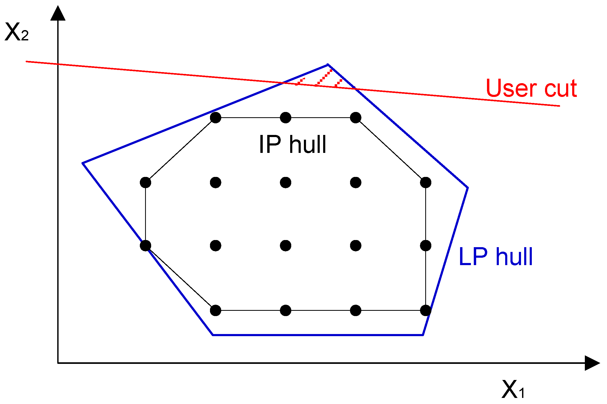
3.1. User Cuts
3.2. Adding N-1 Security Constraints to the UC Problem
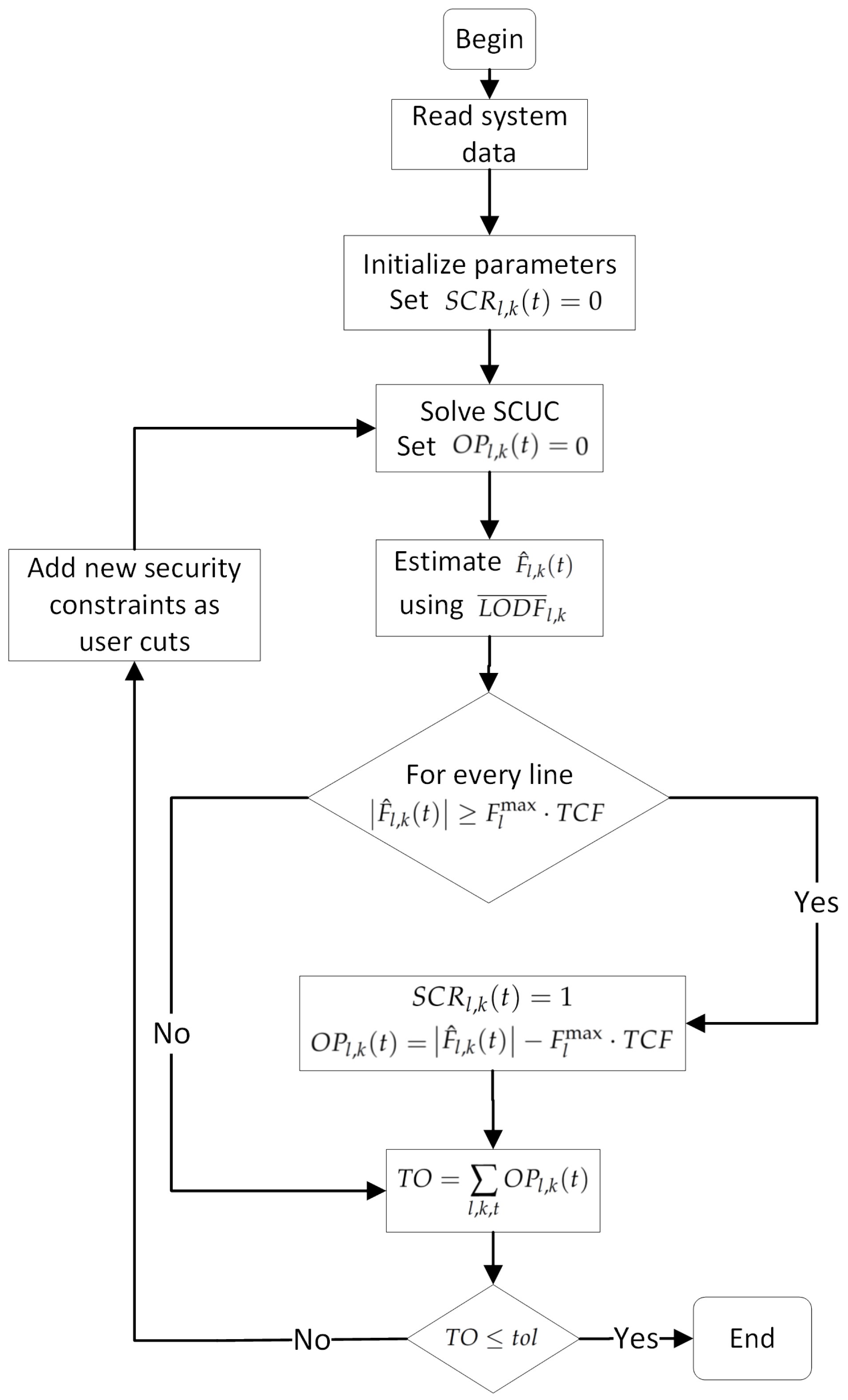
- Step 0: read system data.
- Step 3: Estimate post-contingency power flows as indicated in Equation (35), using the optimal power flows and prior to the contingencies.
- Step 4: verify post-contingency power flow limits in every line l for every period of time t, under every contingency k. If there is an overload in line l, for a contingency k, in the period of time t, assign a value of 1 in the corresponding position of , as indicated in Equation (36).For those lines presenting overloads, the excess value is stored in the Overload Parameter . If there is not an overload in line l, under contingency k in the period of time t the corresponding position of is set to zero as indicated in Equation (37). The sum over the sets of periods, lines and contingencies yields the total overload () of the system as indicated by Equation (38).
- Step 6: check convergence verifying if is lower than a given tolerance (). If it is true, stop the algorithm and report the solution. Otherwise, return to Step 2 introducing user cuts by adding new security constraints through Equation (33). This is done with the values of l, k, and t for which ; which in turn correspond to the positions where .
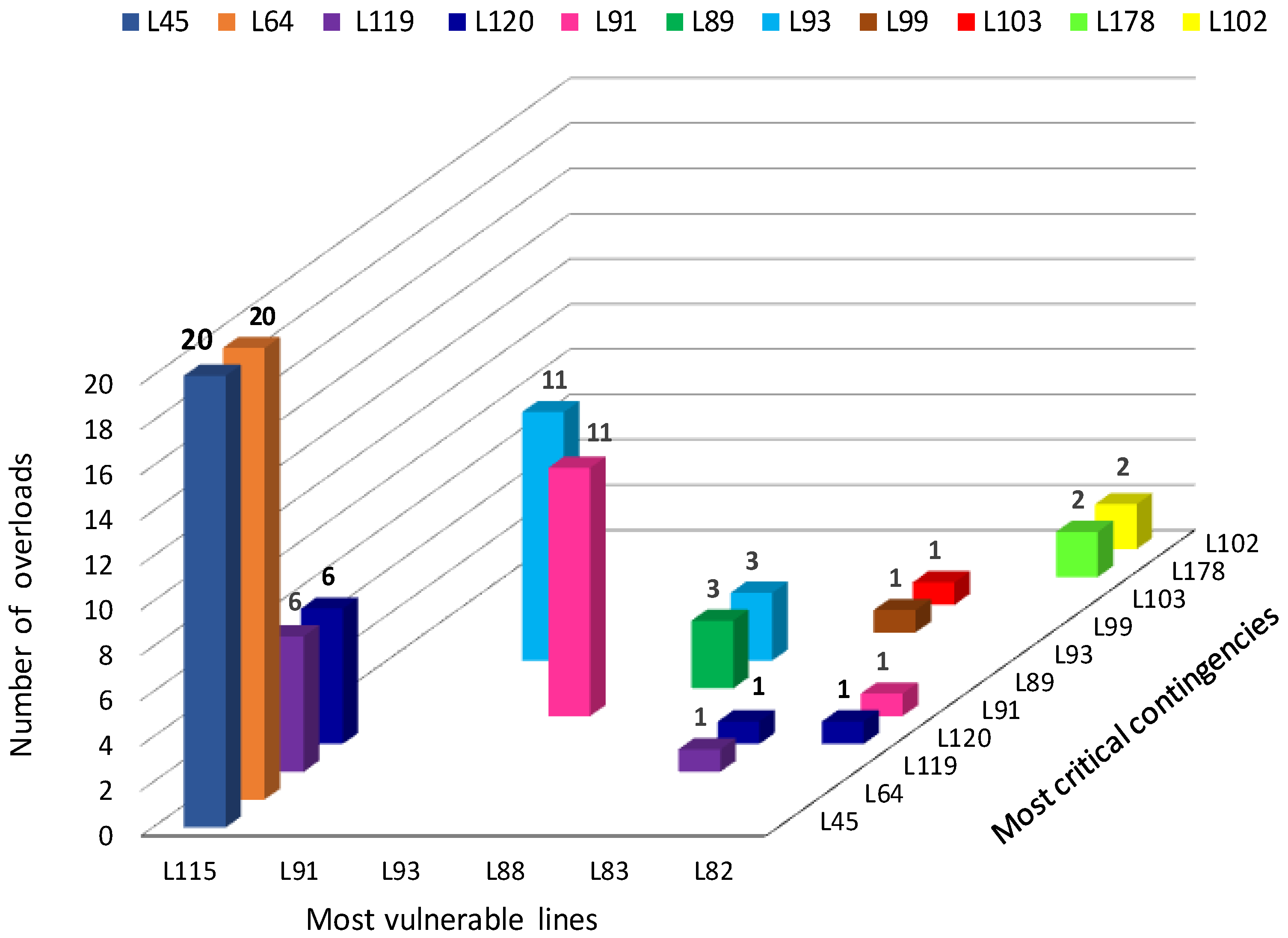
3.3. Identification of Vulnerable Lines and Critical Contingencies
4. Tests and Results
4.1. Impact of Linear Sensitivity Factors in the Performance of the SCUC Problem
4.2. Impact of User Cuts in the Performance of the SCUC Problem
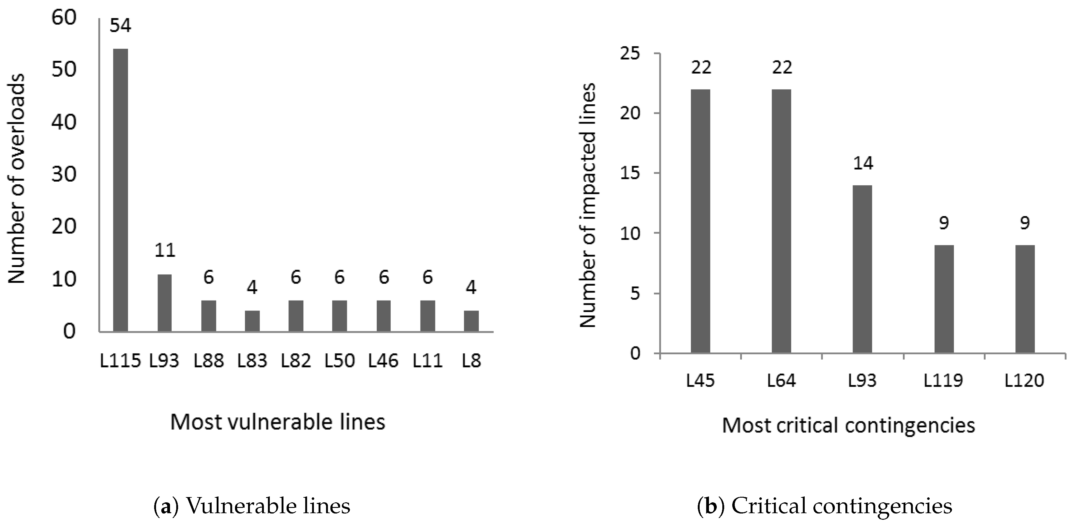
4.3. Most Vulnerable Lines and Critical Contingencies
4.4. Scalability Evaluation
5. Conclusions
Author Contributions
Funding
Acknowledgments
Conflicts of Interest
Abbreviations
| SCOPF | Security-Constraint Optimal Power Flow |
| UC | Unit Commitment |
| SCUC | Security-Constrained Unit Commitment |
| MILP | Mixed-Integer Linear Programming |
| PTDF | Power Transfer Distribution Factors |
| LODF | Line Outage Distribution Factors |
Nomenclature
| b | Index of generating unit cost curve segments, 1 to B |
| i | Index of generating units, 1 to I |
| j | Index of generating unit star-up cost, 1 to K |
| l, k | Index of lines, 1 to L |
| s, m | Index of buses, 1 to S |
| t, tt | Index of hours, 1 to T |
| Fixed production cost of generator ($) | |
| Admittance of line connecting nodes s-m (S) | |
| Demand at bus s (MW) | |
| Minimum down time of generator i (h) | |
| Minimum up time of generator i (h) | |
| Time that generator i has been down before (h) | |
| Time that generator i has been up before (h) | |
| Output if generator i at (MW) | |
| Rated capacity of generator i (MW) | |
| Minimum output of generator i (MW) | |
| Capacity of segment b of the cost curve of generator i (MW) | |
| On-Off status of generator i at (equal to 1 if and 0 otherwise) | |
| Slope of the segment b of the cost curve of generator i ($/MW) | |
| Cost of non-attended demand ($/MW) | |
| Generation map for thermal units | |
| Capacity of the line between nodes s and m (MW) | |
| Capacity of the line between nodes s and m (MW) | |
| Transmission capacity factor | |
| Length of time the generator i must be off at the start time of the planning horizon (h) | |
| Length of time the generator i must be on at the start time of the planning horizon (h) | |
| M | Large number used of linearization - larger than the maximum number of hours a unit can be on or off |
| Ramp-down limit of generator i (MW/h) | |
| Ramp-up limit of generator i (MW/h) | |
| Cost steps in start-up cost curve of generator i ($) | |
| Time steps in start-up cost curve of generator i (h) | |
| Matrix of Power transfer distribution factors | |
| Matrix of Line Outage distribution factors | |
| Security-Constraint Recorder | |
| Vector of vulnerable lines | |
| Vector of critical contingencies | |
| Matrix of vulnerable lines vs. critical contingencies |
| Operating cost of generator i at time t ($) | |
| Generator i down time period counter | |
| Generator i output at time t (MW) | |
| Output of generator i of segment b at time t (MW) | |
| Unserved load at bus s at time t (MW) | |
| Start-up cost of generator i at time t ($) | |
| Binary variable equal to 1 if generator i is started at time t after being off for j hours, and 0 otherwise | |
| Binary variable equal to 1 if the generator i is producing at time t, and 0 otherwise | |
| Binary variable equal to 1 if the generator i is started at the beginning of time t, and 0 otherwise | |
| Binary variable equal to 1 if the generator i is shut down at the beginning of time t, and 0 otherwise | |
| Voltage angle at bus s (rad) | |
| Net power injection in bus s at time t (MW) | |
| Line flow in line l at time t (MW) |
Appendix A.

| Unit | Range | kib | Range | kib | Range | kib |
|---|---|---|---|---|---|---|
| Type | (MW) | ($/MW) | (MW) | ($/MW) | (MW) | ($/MW) |
| 1 | 5.4–7.6 | 29.453 | 7.6–9.8 | 30.120 | 9.8–12 | 30.856 |
| 2 | 8–12 | 28.967 | 12–16 | 29.243 | 16–20 | 29.703 |
| 3 | 26–34 | 28.313 | 34–42 | 29.256 | 43–50 | 30.498 |
| 4 | 40–52 | 18.423 | 52–64 | 19.228 | 64–76 | 20.102 |
| 5 | 40–60 | 17.590 | 60–80 | 18.280 | 80–100 | 18.966 |
| 6 | 54.24–87.83 | 23.810 | 87.83–121.41 | 24.525 | 121.41–155 | 25.240 |
| 7 | 104–135 | 17.193 | 135–166 | 17.708 | 166–197 | 18.225 |
| 8 | 140–210 | 26.213 | 210–280 | 26.708 | 280–350 | 27.200 |
| 9 | 100–200 | 6.961 | 200–300 | 7.230 | 300–400 | 7.499 |
| G | On/off | Init | G | On/off | Init | G | On/off | Init |
|---|---|---|---|---|---|---|---|---|
| 1 | 1 | 20 | 33 | 8 | 20 | 65 | 900 | 20 |
| 2 | 400 | 20 | 34 | 89 | 20 | 66 | 90 | 20 |
| 3 | 220 | 70 | 35 | 66 | 70 | 67 | 789 | 70 |
| 4 | 2 | 0 | 36 | 66 | 0 | 68 | 456 | 0 |
| 5 | 17 | 0 | 37 | 66 | 0 | 69 | 375 | 0 |
| 6 | 4 | 0 | 38 | 66 | 0 | 70 | 375 | 0 |
| 7 | 66 | 0 | 39 | 66 | 0 | 71 | 170 | 0 |
| 8 | 33 | 0 | 40 | 1 | 0 | 72 | 170 | 0 |
| 9 | 11 | 100 | 41 | 1 | 100 | 73 | 170 | 100 |
| 10 | 2 | 90 | 42 | 56 | 90 | 74 | 800 | 90 |
| 11 | 2 | 80 | 43 | 56 | 80 | 75 | 2500 | 80 |
| 12 | 2 | 177 | 44 | 56 | 177 | 76 | 2500 | 177 |
| 13 | 2 | 155 | 45 | 56 | 155 | 77 | 2500 | 155 |
| 14 | 2 | 0 | 46 | 56 | 0 | 78 | 2500 | 0 |
| 15 | 6 | 12 | 47 | 56 | 12 | 79 | 1000 | 12 |
| 16 | 7 | 12 | 48 | 56 | 12 | 80 | 203 | 12 |
| 17 | 8 | 12 | 49 | 98 | 12 | 81 | 600 | 12 |
| 18 | 9 | 0 | 50 | 124 | 0 | 82 | 46 | 0 |
| 19 | 5 | 0 | 51 | 1000 | 0 | 83 | 236 | 0 |
| 20 | 8 | 134 | 52 | 1000 | 134 | 84 | 236 | 134 |
| 21 | 8 | 123 | 53 | 1000 | 123 | 85 | 64 | 123 |
| 22 | 8 | 0 | 54 | 50 | 0 | 86 | 6 | 0 |
| 23 | 8 | 377 | 55 | 50 | 377 | 87 | 8 | 377 |
| 24 | 8 | 47 | 56 | 90 | 47 | 88 | 90 | 47 |
| 25 | 8 | 48 | 57 | 900 | 48 | 89 | 5 | 48 |
| 26 | 8 | 0 | 58 | 900 | 0 | 90 | 6 | 0 |
| 27 | 8 | 0 | 59 | 900 | 0 | 91 | 7 | 0 |
| 28 | 8 | 50 | 60 | 900 | 50 | 92 | 8 | 50 |
| 29 | 8 | 50 | 61 | 900 | 50 | 93 | 9 | 50 |
| 30 | 8 | 150 | 62 | 900 | 150 | 94 | 7 | 150 |
| 31 | 8 | 0 | 63 | 900 | 0 | 95 | 66 | 0 |
| 32 | 8 | 0 | 64 | 900 | 0 | 96 | 55 | 0 |
References
- Song, M.; Amelin, M. Purchase Bidding Strategy for a Retailer With Flexible Demands in Day-Ahead Electricity Market. IEEE Trans. Power Syst. 2017, 32, 1839–1850. [Google Scholar] [CrossRef]
- Lee, H.; Tekin, C.; van der Schaar, M.; Lee, J. Adaptive Contextual Learning for Unit Commitment in Microgrids with Renewable Energy Sources. IEEE J. Sel. Top. Signal Process. 2018, 12, 688–702. [Google Scholar] [CrossRef]
- Li, N.; Hedman, K.W. Economic Assessment of Energy Storage in Systems With High Levels of Renewable Resources. IEEE Trans. Sustain. Energy 2015, 6, 1103–1111. [Google Scholar] [CrossRef]
- Carrión, M.; Zárate-Miñano, R.; Domínguez, R. A Practical Formulation for Ex-Ante Scheduling of Energy and Reserve in Renewable-Dominated Power Systems: Case Study of the Iberian Peninsula. Energies 2018, 11, 1939. [Google Scholar] [CrossRef]
- Pozo, D.; Contreras, J.; Sauma, E.E. Unit Commitment With Ideal and Generic Energy Storage Units. IEEE Trans. Power Syst. 2014, 29, 2974–2984. [Google Scholar] [CrossRef]
- Lv, M.; Lou, S.; Wu, Y.; Miao, M. Unit Commitment of a Power System Including Battery Swap Stations Under a Low-Carbon Economy. Energies 2018, 11, 1898. [Google Scholar] [CrossRef]
- Pandžić, H.; Dvorkin, Y.; Qiu, T.; Wang, Y.; Kirschen, D.S. Toward Cost-Efficient and Reliable Unit Commitment Under Uncertainty. IEEE Trans. Power Syst. 2016, 31, 970–982. [Google Scholar] [CrossRef]
- Zhao, B.; Conejo, A.J.; Sioshansi, R. Unit Commitment Under Gas-Supply Uncertainty and Gas-Price Variability. IEEE Trans. Power Syst. 2017, 32, 2394–2405. [Google Scholar] [CrossRef]
- Tejada-Arango, D.A.; Sánchez-Martın, P.; Ramos, A. Security Constrained Unit Commitment Using Line Outage Distribution Factors. IEEE Trans. Power Syst. 2018, 33, 329–337. [Google Scholar] [CrossRef]
- Zhai, Q.; Guan, X.; Cheng, J.; Wu, H. Fast Identification of Inactive Security Constraints in SCUC Problems. IEEE Trans. Power Syst. 2010, 25, 1946–1954. [Google Scholar] [CrossRef]
- Fu, Y.; Shahidehpour, M.; Li, Z. Long-term security-constrained unit commitment: hybrid Dantzig-Wolfe decomposition and subgradient approach. IEEE Trans. Power Syst. 2005, 20, 2093–2106. [Google Scholar] [CrossRef]
- Al-Agtash, S. Hydrothermal scheduling by augmented Lagrangian: consideration of transmission constraints and pumped-storage units. IEEE Trans. Power Syst. 2001, 16, 750–756. [Google Scholar] [CrossRef]
- Guan, X.; Guo, S.; Zhai, Q. The conditions for obtaining feasible solutions to security-constrained unit commitment problems. IEEE Trans. Power Syst. 2005, 20, 1746–1756. [Google Scholar] [CrossRef]
- Lu, B.; Shahidehpour, M. Unit commitment with flexible generating units. IEEE Trans. Power Syst. 2005, 20, 1022–1034. [Google Scholar] [CrossRef]
- Martinez-Crespo, J.; Usaola, J.; Fernandez, J.L. Security-constrained optimal generation scheduling in large-scale power systems. IEEE Trans. Power Syst. 2006, 21, 321–332. [Google Scholar] [CrossRef]
- Fu, Y.; Shahidehpour, M. Fast SCUC for Large-Scale Power Systems. IEEE Trans. Power Syst. 2007, 22, 2144–2151. [Google Scholar] [CrossRef]
- Alemany, J.; Magnago, F. Benders decomposition applied to security constrained unit commitment: Initialization of the algorithm. Int. J. Electr. Power Energy Syst. 2015, 66, 53–66. [Google Scholar] [CrossRef]
- Guan, X.; Zhai, Q.; Papalexopoulos, A. Optimization based methods for unit commitment: Lagrangian relaxation versus general mixed integer programming. In Proceedings of the 2003 IEEE Power Engineering Society General Meeting (IEEE Cat. No.03CH37491), Toronto, ON, Canada, 13–17 July 2003; Volume 2, pp. 1095–1100. [Google Scholar] [CrossRef]
- Bragin, M.A.; Luh, P.B.; Yan, J.H.; Stern, G.A. Novel exploitation of convex hull invariance for solving unit commitment by using surrogate Lagrangian relaxation and branch-and-cut. In Proceedings of the 2015 IEEE Power Energy Society General Meeting, Denver, Colorado, 26–30 July 2015; pp. 1–5. [Google Scholar] [CrossRef]
- Swarup, K.S.; Yamashiro, S. Unit commitment solution methodology using genetic algorithm. IEEE Trans. Power Syst. 2002, 17, 87–91. [Google Scholar] [CrossRef]
- Senjyu, T.; Yamashiro, H.; Shimabukuro, K.; Uezato, K.; Funabashi, T. Fast solution technique for large-scale unit commitment problem using genetic algorithm. IEE Proc. Gener. Trans. Distrib. 2003, 150, 753–760. [Google Scholar] [CrossRef]
- Aghdam, F.H.; Hagh, M.T. Security Constrained Unit Commitment (SCUC) formulation and its solving with Modified Imperialist Competitive Algorithm (MICA). J. King Saud Univ. Eng. Sci. 2017. [Google Scholar] [CrossRef]
- Roque, L.A.C.; Fontes, D.B.M.M.; Fontes, F.A.C.C. A Metaheuristic Approach to the Multi-Objective Unit Commitment Problem Combining Economic and Environmental Criteria. Energies 2017, 10, 2029. [Google Scholar] [CrossRef]
- Jo, K.H.; Kim, M.K. Improved Genetic Algorithm-Based Unit Commitment Considering Uncertainty Integration Method. Energies 2018, 11, 1387. [Google Scholar] [CrossRef]
- Zhao, J.; Liu, S.; Zhou, M.; Guo, X.; Qi, L. An Improved Binary Cuckoo Search Algorithm for Solving Unit Commitment Problems: Methodological Description. IEEE Access 2018, 6, 43535–43545. [Google Scholar] [CrossRef]
- Singhal, P.K.; Naresh, R.; Sharma, V. Binary fish swarm algorithm for profit-based unit commitment problem in competitive electricity market with ramp rate constraints. IET Gener. Trans. Distrib. 2015, 9, 1697–1707. [Google Scholar] [CrossRef]
- Trivedi, A.; Srinivasan, D.; Pal, K.; Saha, C.; Reindl, T. Enhanced Multiobjective Evolutionary Algorithm Based on Decomposition for Solving the Unit Commitment Problem. IEEE Trans. Ind. Inform. 2015, 11, 1346–1357. [Google Scholar] [CrossRef]
- Arora, V.; Chanana, S. Solution to unit commitment problem using Lagrangian relaxation and Mendel’s GA method. In Proceedings of the 2016 International Conference on Emerging Trends in Electrical Electronics Sustainable Energy Systems (ICETEESES), Sultanpur, India, 11–12 March 2016; pp. 126–129. [Google Scholar] [CrossRef]
- Pandžić, H.; Qiu, T.; Kirschen, D.S. Comparison of state-of-the-art transmission constrained unit commitment formulations. In Proceedings of the 2013 IEEE Power Energy Society General Meeting, Vancouver, BC, USA, 21–25 July 2013; pp. 1–5. [Google Scholar] [CrossRef]
- Bhardwaj, A.; Kamboj, V.K.; Shukla, V.K.; Singh, B.; Khurana, P. Unit commitment in electrical power system-a literature review. In Proceedings of the 2012 IEEE International Power Engineering and Optimization Conference, Melaka, Malaysia, 6–7 June 2012; pp. 275–280. [Google Scholar] [CrossRef]
- Zheng, Q.P.; Wang, J.; Liu, A.L. Stochastic Optimization for Unit Commitment—A Review. IEEE Trans. Power Syst. 2015, 30, 1913–1924. [Google Scholar] [CrossRef]
- Jurković, K.; Pandšić, H.; Kuzle, I. Review on unit commitment under uncertainty approaches. In Proceedings of the 2015 38th International Convention on Information and Communication Technology, Electronics and Microelectronics (MIPRO), Opatija, Croatia, 25–29 May 2015; pp. 1093–1097. [Google Scholar] [CrossRef]
- Wu, H.; Guan, X.; Zhai, Q.; Ye, H. A Systematic Method for Constructing Feasible Solution to SCUC Problem With Analytical Feasibility Conditions. IEEE Trans. Power Syst. 2012, 27, 526–534. [Google Scholar] [CrossRef]
- Ardakani, A.J.; Bouffard, F. Identification of Umbrella Constraints in DC-Based Security-Constrained Optimal Power Flow. IEEE Trans. Power Syst. 2013, 28, 3924–3934. [Google Scholar] [CrossRef]
- Capitanescu, F.; Glavic, M.; Ernst, D.; Wehenkel, L. Contingency Filtering Techniques for Preventive Security-Constrained Optimal Power Flow. IEEE Trans. Power Syst. 2007, 22, 1690–1697. [Google Scholar] [CrossRef]
- Fu, Y.; Shahidehpour, M.; Li, Z. Security-constrained unit commitment with AC constraints. IEEE Trans. Power Syst. 2005, 20, 1538–1550. [Google Scholar] [CrossRef]
- Fu, Y.; Shahidehpour, M.; Li, Z. AC contingency dispatch based on security-constrained unit commitment. IEEE Trans. Power Syst. 2006, 21, 897–908. [Google Scholar] [CrossRef]
- Bragin, M.A.; Luh, P.B.; Yan, J.H.; Stern, G.A. An efficient approach for Unit Commitment and Economic Dispatch with combined cycle units and AC Power Flow. In Proceedings of the 2016 IEEE Power and Energy Society General Meeting (PESGM), Boston, MA, USA, 17–21 July 2016; pp. 1–5. [Google Scholar] [CrossRef]
- Guler, T.; Gross, G.; Liu, M. Generalized Line Outage Distribution Factors. IEEE Trans. Power Syst. 2007, 22, 879–881. [Google Scholar] [CrossRef]
- Leveringhaus, T.; Hofmann, L. Comparison of methods for state prediction: Power Flow Decomposition (PFD), AC Power Transfer Distribution factors (AC-PTDFs), and Power Transfer Distribution factors (PTDFs). In Proceedings of the 2014 IEEE PES Asia-Pacific Power and Energy Engineering Conference (APPEEC), Kowloon, Hong Kong, 7–10 December 2014; pp. 1–6. [Google Scholar] [CrossRef]
- Song, C.S.; Park, C.H.; Yoon, M.; Jang, G. Implementation of PTDFs and LODFs for Power System Security. J. Int. Counc. Electr. Eng. 2011, 1, 49–53. [Google Scholar] [CrossRef]
- Chen, Y.C.; Domínguez-García, A.D.; Sauer, P.W. Measurement-Based Estimation of Linear Sensitivity Distribution Factors and Applications. IEEE Trans. Power Syst. 2014, 29, 1372–1382. [Google Scholar] [CrossRef]
- Eslami, M.; Moghadam, H.A.; Zayandehroodi, H.; Ghadimi, N. A New Formulation to Reduce the Number of Variables and Constraints to Expedite SCUC in Bulky Power Systems. Proc. Natl. Acad. Sci. India Sect. A Phys. Sci. 2018. [Google Scholar] [CrossRef]
- Wood, A.J.; Wollenberg, B.F.; Sheble, G.B. Power Generation, Operation, and Control; Wiley-IEEE Press: Piscataway, NJ, USA, 2013. [Google Scholar]
- Pandzic, H.; Dvorkin, Y.; Qiu, T.; Wang, Y.; Kirschen, D. Unit Commitment under Uncertainty—GAMS Models; Library of the Renewable Energy Analysis Lab (REAL), University of Washington: Seattle, DC, USA; Available online: https://www2.ee.washington.edu/research/real/gams_code.html (accessed on 27 February 2019).
- IBM®-IBM Knowledge Center. Differences between User Cuts and Lazy Constraints. 2014. Available online: https://www.ibm.com/support/knowledgecenter/SSSA5P_12.6.1/ilog.odms.cplex.help/CPLEX/UsrMan/topics/progr_adv/usr_cut_lazy_constr/04_diffs.html (accessed on 15 February 2019).
- IceMerman. Unit Commitment with User Cuts Implementation. 2019. Available online: https://github.com/IceMerman/SCUC-UserCuts (accessed on 1 March 2019).


| Formulation | Description |
|---|---|
| A | Conventional network formulation given by Equations (9)–(29) Contingency constraints computed using LODF (Equation (33)) |
| B | Network formulation using PTDF (Equations (26) to (29) are replaced by Equations (30) to (32) Contingency constraints computed using LODF (Equation (33) |
| C | Network formulation using PTDF (Equations (26) to (29) are replaced by Equations (30) to (32) Contingency constraints computed using LODF (Equation (33) Implementation of user cuts as described in Section 3.1 |
| Formulation | Objective Function [M$] | Time [s] | inGAP | outGAP | ||||
|---|---|---|---|---|---|---|---|---|
| TCF = 1 | TCF = | TCF = 1 | TCF = | TCF = 1 | TCF = | TCF = 1 | TCF = | |
| A | 1220 | 519 | ||||||
| B | 1209 | 345 | ||||||
| C | 169 | 321 | ||||||
| B* | 495 | 687 | ||||||
| Iteration | Added Constraints N-1 | Elapsed Time of Simulation [s] | Objective Function [M$] |
|---|---|---|---|
| 1 | - | 25 | |
| 2 | 68 | 66 | |
| 3 | 21 | 87 | |
| 4 | 7 | 53 | |
| 5 | 27 | 57 | |
| 6 | 21 | 33 | |
| total | 144 | 321 | - |
| Formulation | Objective Function [M$] | Time [s] | inGAP | outGAP |
|---|---|---|---|---|
| B | 4.8748 | 7494.001 | 0.01 | 0.00178 |
| C | 4.8701 | 209.687 | 0.01 | 0.00100 |
© 2019 by the authors. Licensee MDPI, Basel, Switzerland. This article is an open access article distributed under the terms and conditions of the Creative Commons Attribution (CC BY) license (http://creativecommons.org/licenses/by/4.0/).
Share and Cite
Marín-Cano, C.C.; Sierra-Aguilar, J.E.; López-Lezama, J.M.; Jaramillo-Duque, Á.; Villa-Acevedo, W.M. Implementation of User Cuts and Linear Sensitivity Factors to Improve the Computational Performance of the Security-Constrained Unit Commitment Problem. Energies 2019, 12, 1399. https://doi.org/10.3390/en12071399
Marín-Cano CC, Sierra-Aguilar JE, López-Lezama JM, Jaramillo-Duque Á, Villa-Acevedo WM. Implementation of User Cuts and Linear Sensitivity Factors to Improve the Computational Performance of the Security-Constrained Unit Commitment Problem. Energies. 2019; 12(7):1399. https://doi.org/10.3390/en12071399
Chicago/Turabian StyleMarín-Cano, Cristian Camilo, Juan Esteban Sierra-Aguilar, Jesús M. López-Lezama, Álvaro Jaramillo-Duque, and Walter M. Villa-Acevedo. 2019. "Implementation of User Cuts and Linear Sensitivity Factors to Improve the Computational Performance of the Security-Constrained Unit Commitment Problem" Energies 12, no. 7: 1399. https://doi.org/10.3390/en12071399
APA StyleMarín-Cano, C. C., Sierra-Aguilar, J. E., López-Lezama, J. M., Jaramillo-Duque, Á., & Villa-Acevedo, W. M. (2019). Implementation of User Cuts and Linear Sensitivity Factors to Improve the Computational Performance of the Security-Constrained Unit Commitment Problem. Energies, 12(7), 1399. https://doi.org/10.3390/en12071399