Neural Network-Based Modeling of Electric Vehicle Energy Demand and All Electric Range ^†

Abstract

A deep neural network-based approach of energy demand modeling of electric vehicles (EV) is proposed in this paper. The model-based prediction of energy demand is based on driving cycle time series used as a model input, which is properly preprocessed and transformed into 1D or 2D static maps to serve as a static input to the neural network. Several deep feedforward neural network architectures are considered for this application along with different model input formats. Two energy demand models are derived, where the first one predicts the battery state-of-charge and fuel consumption at destination for an extended range electric vehicle, and the second one predicts the vehicle all-electric range. The models are validated based on a separate test dataset when compared to the one used in neural network training, and they are compared with the traditional response surface approach to illustrate effectiveness of the method proposed.

1. Introduction

In the last decade, there has been a trend of connecting the electric energy and transport systems through the appearance of electric vehicles (EV) and the need for their charging. Increased proliferation of EVs will require implementation of suitable load management procedures for electric grids in terms of applying optimal charging strategies to EV fleets, which would be facilitated by use of various Vehicle-to-Infrastructure (V2I) and Vehicle-to-Grid (V2G) communication methods [1]. In order to provide optimal EV fleet charging management within smart grids, there is a necessity for accurate models aimed at predicting the energy demand of each individual EV in the fleet, including prediction of battery state of charge (SoC) at destination (e.g., at the charging station). Such energy demand models can be used to optimize routes and charging schedules in order to ultimately minimize fuel- and electricity consumption-related costs [2,3].

The energy demand can be predicted based on a precise EV powertrain model, where each sub-component is modeled separately [4]. However, building of such models can be time consuming and thus impractical to use in the case of fleets where new vehicles are frequently added. Also, performing EV simulations within an optimization-based charging/routing management framework can be impractical from the standpoint of computational efficiency. Another possibility for modeling the EV energy demand relates to use of computationally efficient response surface-based method [5], where the model parameterization can be conducted off-line based on precise EV model simulations over recorded or synthetic driving cycles, or GPS- and energy consumption-related data that are typically collected in delivery fleets [6]. However, the drawbacks of this approach include: (i) complexity of the selection of significant driving cycle features to serve as inputs to the model [7], (ii) selection of an appropriate regression model, and (iii) the inflexibility of transferring the knowledge gained for one vehicle to another one. Furthermore, some recent studies related to transport energy demand modeling involve artificial neural networks (NN) for long-term energy demand forecasting, and are performed on national level by considering various socio-economic and transport related indicators [8,9,10,11]. Other studies are either related to short-term predictions of EV energy consumption in real time [12,13], EV energy consumption on the individual segments of the road network [2], or are based on a single parameter which accounts for the dependence of vehicle energy consumption on vehicle mass and driving cycle [14].

The above drawbacks and limitations can be overcome by applying data-driven deep learning methods, which are usually implemented through using a NN architecture. The main advantage of these deep computational models is in their ability to learn features from given inputs automatically (i.e., no manual feature extraction is needed), and to transfer knowledge from the base task to other related tasks by means of transfer learning. Deep learning models are especially well-suited for image classification tasks (e.g., convolutional neural networks—CNNs), which use convolutions instead of general matrix multiplication, and possess the translation invariance property) [15]. One of the most popular classification challenges is ImageNet Large Scale Visual Recognition Competition (ILVRSC), which involves the task of classifying images into one of 1000 categories, while offering a training dataset containing 1.2 million images. The most accurate models which have participated on the recent ILVRSC challenges are AlexNet, Oxford VGG model, GoogLeNet (Inception module) [16], and Microsoft ResNet with a leading score of top-5 error rate (i.e., the target label is one of top five predictions) equal to 3.57% [17].

Significant deep learning achievements have been reached in autonomous vehicle-related applications, whose key components are perception modules controlled by an underlying deep NN. These deep NN models take inputs from different sensors including cameras, light detection and ranging sensors, and infrared sensors and output the information necessary to maneuver a vehicle safely under given conditions [18,19]. Apart from perception applications in autonomous vehicles, NNs are also widely used in other different transport-related applications. For instance, in [20], a deep NN is used for prediction of specific driver speed profiles, while in [21,22] NN-based models are used for prediction of traffic speed on specific road segments. A similar approach is proposed in [23], where a NN-based model is used for on-line identification of road type and traffic congestion levels, with the purpose of improving the vehicle power management system. Furthermore, NNs can also be used for forecasting the number of electric vehicles (EVs) in the city or state [24], or the number of passengers inside the vehicle [25]. Deep NN model-based methods are used for EV charging management in [26,27]. In [28,29,30] various NN architectures were developed and applied to estimate the actual EV battery SoC with high precision.

According to the best of the authors’ knowledge, EV energy demand modeling based on deep NNs and known driving cycle features as inputs has not been considered in the literature so far. To fill the gap, this paper proposes a novel data-driven approach of EV energy demand modeling based on deep neural networks. The approach is particularly suitable for cases when large driving cycle datasets are available, as in the case of vehicle fleets equipped with GPS/GPRS tracking equipment. A preprocessing method for transforming time- and distance-varying driving cycles into 1D or 2D static maps is proposed, in order to make them appropriate for use as inputs to neural networks. Several deep feedforward artificial neural network architectures including multilayer perceptrons (MLPs) and CNNs have been considered and analyzed along with three different model input formats (see an illustration in Figure 1). Necessary driving energy demand data is generated through numerous simulations of an extended range electric vehicle (EREV) model over a wide set of driving cycles recorded for a delivery vehicle fleet. Two energy demand-related models are derived based on the generated data, in order to predict: (i) the battery SoC and fuel consumption at the end of driving cycle (i.e., at destination), and (ii) all-electric range (i.e., the distance that can be travelled in pure electric driving prior to a hybrid driving mode being engaged; AER). The derived models can be applied in different off-line energy demand studies (e.g., in energy planning), as well as in on-line energy consumption prediction and energy management strategies.

The main contributions of the paper include: (i) proposing the driving cycle preprocessing method that provides proper inputs to NNs and accounts for the initial battery SoC value, (ii) recommending the most appropriate combination of NN architecture and driving cycle input format, and (iii) conducting a comparative performance analysis of the proposed NN-based method and the traditional response surface modeling approach.

2. Driving Cycle Data Preprocessing

This section first briefly describes the process of driving cycle data collection based on GPS/GPRS tracking technology applied on a set of ten mid-size delivery trucks [6]. A method for preprocessing of driving cycles is then elaborated, along with definition of several resulting formats of processed driving cycles aimed to be used as inputs to a feedforward NN.

2.1. Delivery Vehicle Fleet Description and Driving Data Collection

The delivery vehicle fleet considered in this paper consists of a set of ten mid-size MAN-TGM 15.240 trucks. The driving missions of these trucks relate to delivery of goods from a main distribution center to sales centers. The truck loading capacity is 7460 kg and the empty vehicle mass is 7860 kg. The vehicle is propelled by a diesel engine with the maximum power of 176 kW. The vehicle maximum velocity equals 90 km/h.

Driving data have been collected by using the vehicle tracking equipment based on GPS and GPRS technology. The driving data were recorded continuously, i.e., 24 h a day, over a time period of three months (91 days). The data sampling time was set to 1 s. Apart from the GPS-related data, an additional set of data from the vehicle controller area network (CAN) bus were acquired (e.g., engine rotational speed and cumulative fuel consumption). The recorded GPS data include the following information: vehicle ID number, timestamps, vehicle velocity, vehicle position (longitude and latitude), and altitude. A total of 2286 driving cycles were extracted from the overall recorded dataset, where each driving cycle corresponds to a single driving mission determined by the time interval between vehicle departure from and its arrival back to the distribution center.

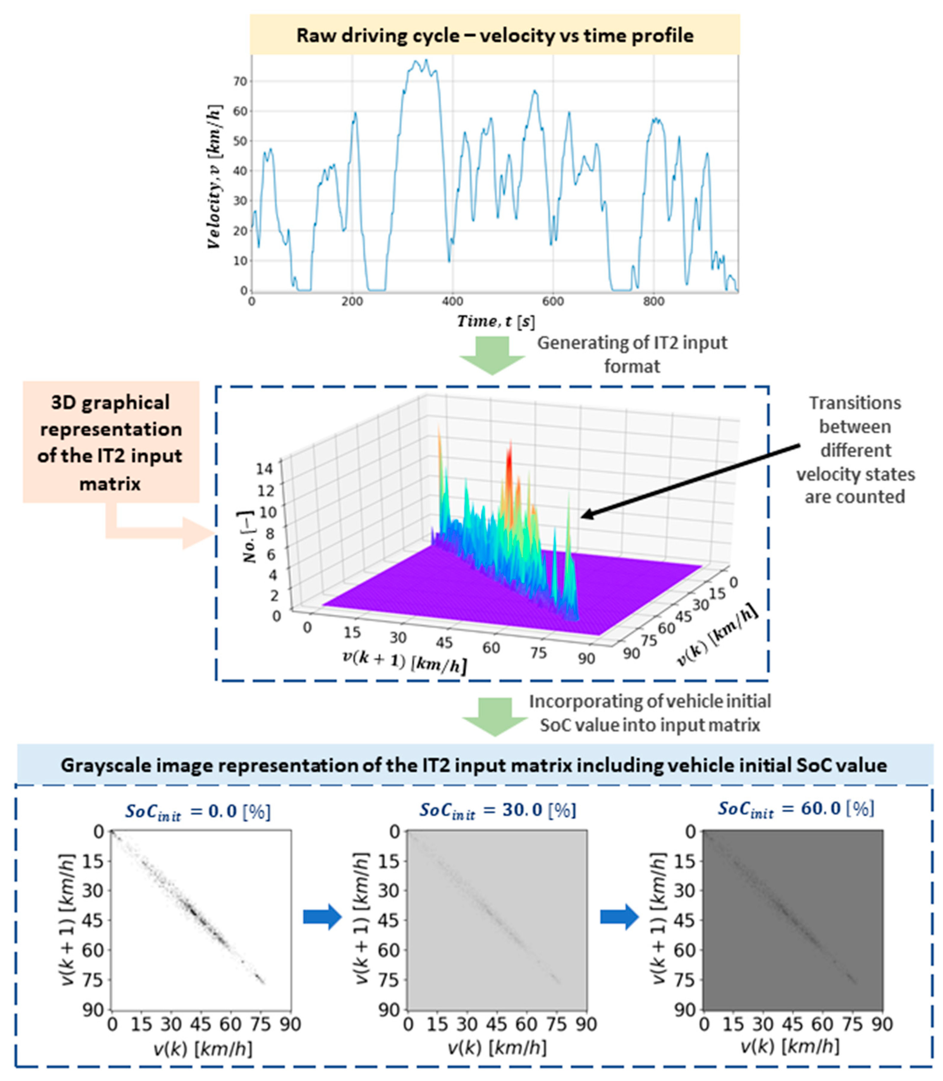
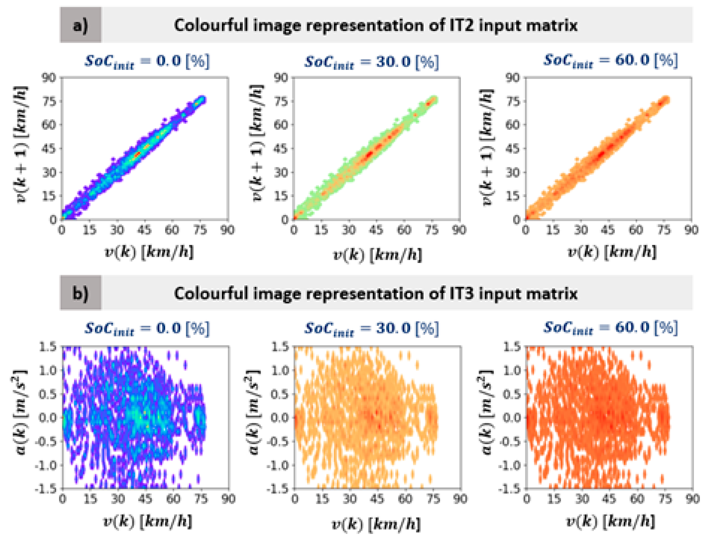
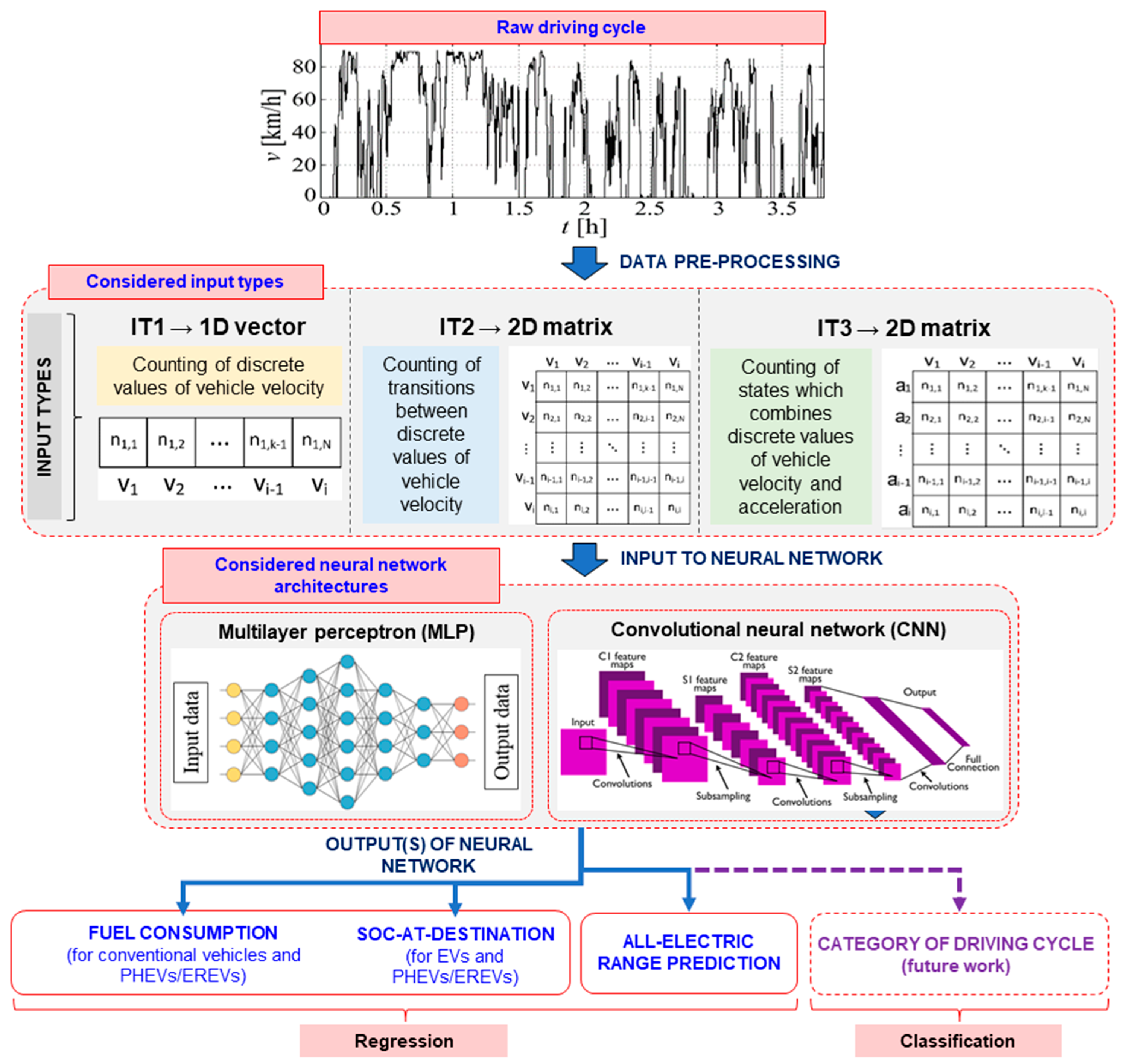
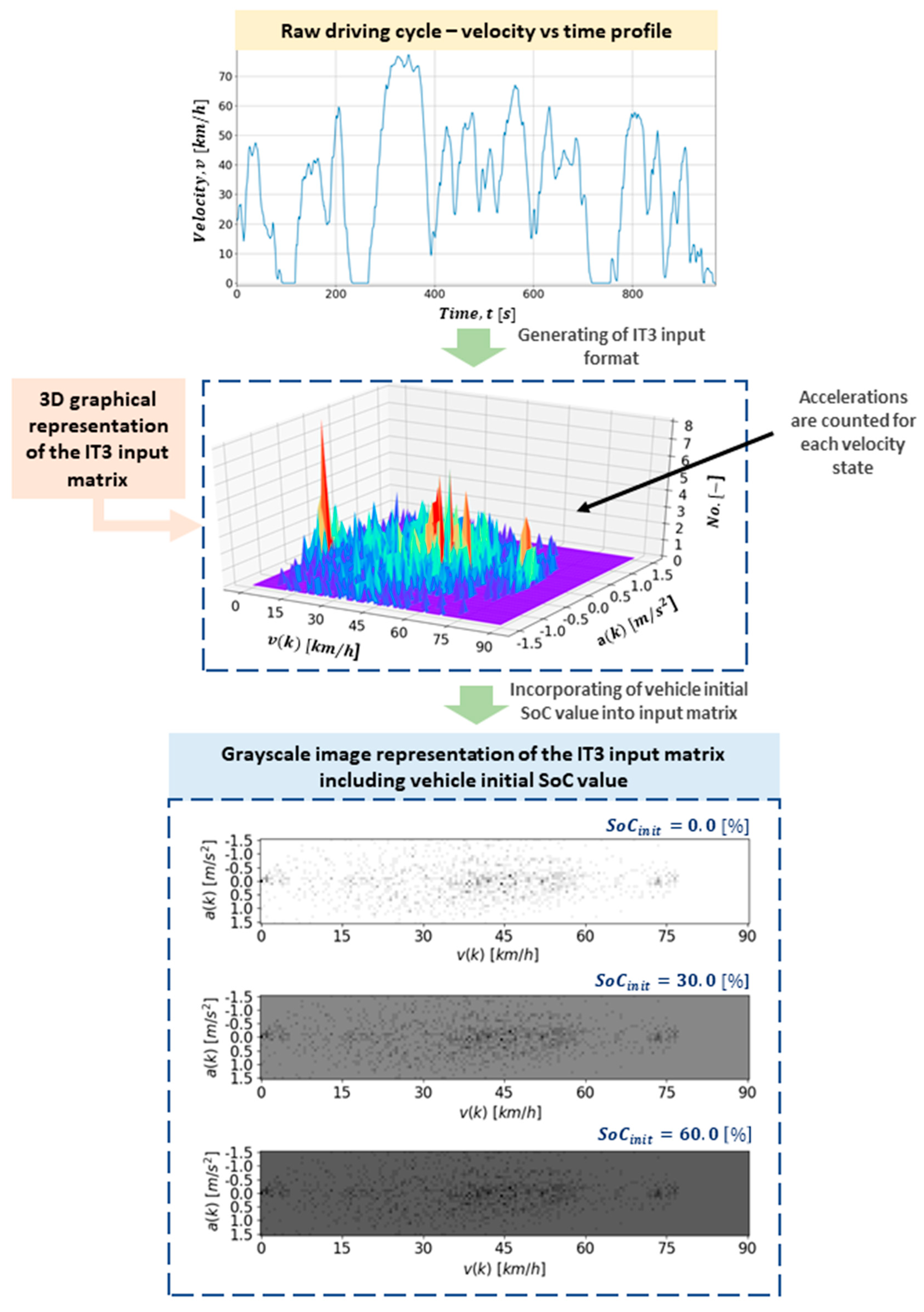
2.2. Preprocessing of Driving Cycles to Serve as Neural Network Inputs

The longitudinal dynamics of vehicle is described by the following equations:

$${\tau }_L=r\left[m_v\frac{d{v}_v}{dt}+m_{v}g\sin \alpha +m_{v}g{R}_o\cos \alpha +0.5{\rho }_{air}{C}_d{A}_f{v}_v^2\right],$$

(1)

$${\omega }_L=\frac{v_v}{r},$$

(2)

where τ_L and ω_L are the total wheel torque and angular velocity, respectively, v_v is the vehicle velocity, m_v is the vehicle mass, r is the effective tire radius, g is the gravitational acceleration, α is the road slope, R_o is the tire rolling coefficient, ρ_air is the air density with the standard value of 1.225 kg/m³, C_d is the vehicle aerodynamic drag coefficient, and A_f is a vehicle frontal cross-section area. The demanded energy on wheels can be calculated as:

$$E_{wheel}={{\displaystyle \int }}_{t=0}^{T_f}{\omega }_L{\tau }_{L}dt,$$

(3)

where T_f represents the driving cycle duration. By inspecting Equations (1)–(3), it can be concluded that the significant variables from the perspective of energy demand are: (i) vehicle velocity v_v, (ii) vehicle acceleration a = dv_v/dt, (iii) road slope α, and (iv) vehicle mass m_v. In this paper only vehicle velocity v_v and acceleration dv_v/dt are taken into account when generating inputs to considered NNs.

Since driving cycles can be variable both in time and travelled distance, and the feedforward NNs are supposed to be fed by static inputs of constant dimensions, driving cycle preprocessing is needed. Because different NN architectures require different input formats (see Figure 1 and Section 4), three input types (IT) of NNs labeled as IT1, IT2, and IT3 are proposed (

Table 1. Description of IT1, IT2 and IT3 input formats.

Label	Type	Dimension	Velocity [km/h]		Acceleration [m/s2]		Incorporating of Initial SoC Value
			Range	Resolution	Range	Resolution
IT1	Vector	1 × 182	[0, 90]	0.5	/	/	append
IT2	Matrix	91 × 91	[0, 90]	1.0	/	/	addition
IT3	Matrix	31 × 182	[0, 90]	0.5	[−1.5, 1.5]	0.1	addition

). The input IT1 refers to 1D vector of counted velocity states in range of 0 to 90 km/h, with resolution of 0.5 km/h. The input IT2 refers to 2D matrix of counted transitions between the different velocity states, where velocity range is equal as in the case of IT1 input, but with the resolution of 1 km/h. Here, the information of vehicle acceleration is included indirectly through counting of transitions between discrete values of vehicle velocities. The input IT3 refers to 2D matrix of counted accelerations for each velocity state defined in IT1, where the acceleration range and resolution are equal to ±1.5 m/s² and 0.1 m/s², respectively. In this case, the information on vehicle acceleration is directly included. It should be mentioned that regardless of input type, by counting the discrete values of vehicle velocities for the given fixed sampling time, the information on travelled distance is accounted for implicitly (note that this information highly impacts the energy demand [4]).

Apart from the driving cycle-related velocity and acceleration information, the initial battery SoC value (SoC_init) needs to be included in the NN input to be able to predict the energy demand (e.g., SoC at destination). Various methods have been considered within this study, such as appending the input vector/matrix by SoC_init, multiplying each element of input matrix by SoC_init, etc. A simple addition of initial SoC to the overall input matrix has been found to be the best approach in terms of NN prediction accuracy. Exceptionally, in the IT1 case the initial SoC value is appended to the input vector. The addition of vehicle initial SoC value for the cases of matrix input formats (IT2 and IT3) can be visualized as a magnification of grey intensity in the graphical representation of the matrix, as illustrated in Figure 2 for the case of IT2 and initial SoC values ranging from 0.3 to 0.6. This figure shows that IT2 has very sparse structure (i.e., useful information just around diagonal positions), which affects the quality of recognition of sample features, while requiring long learning time of NN due to high dimension of input matrix. This difficulty is effectively overcome in the case of IT3, which is characterized by the reduced input dimensions (see Table 1), far less sparse structure (see Figure 3), and directly included acceleration information. The reduced input dimension makes the NN training process less time consuming due to a lower number of trainable parameters. For the sake of better visualization of addition of initial SoC to 2D inputs in the case of IT2 and IT3, the inputs are shown as contour plots in Figure 4.

The procedure for generating inputs for NN-based energy demand models for the purpose of their training (i.e., parameterization) and testing is as follows: (i) splitting of overall driving cycle dataset into two distinctive groups, where 85% of data is used for training of NNs, while remaining 15% of data is employed for model testing, (ii) extracting of vehicle velocity and acceleration values from the driving cycle data; (iii) counting of the states including discrete values of vehicle velocity (and acceleration) and transitions between states and storing them into 1D or 2D static maps depending on the required NN input format (i.e., IT1, IT2 or IT3), and (iv) adding the initial SoC value SoC_init into the given input format.

3. Generating Energy Demand Data

This section describes simulation data generated for the purpose of parameterization and validation of NN-based energy demand models. The first subsection deals with building up a simulation model of delivery EREV, which is executed over the recorded driving cycles (described in Section 2.1) for different initial SoC values. The obtained simulation results including fuel consumption, SoC at destination and AER are analyzed in the second subsection.

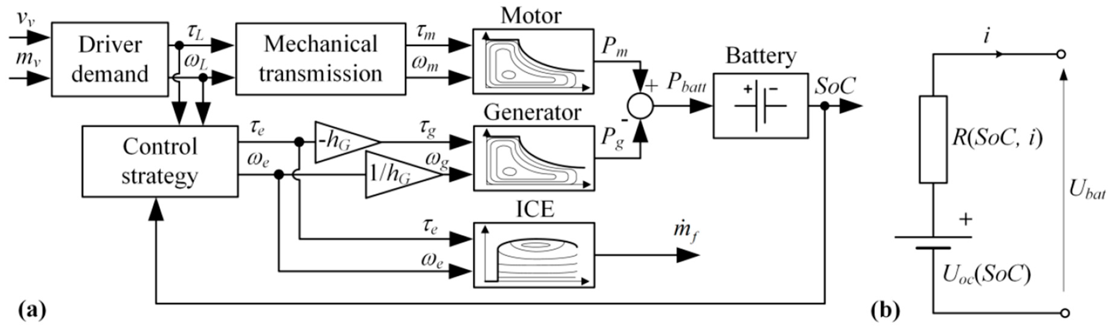
3.1. Modeling of Delivery EREV

A delivery EREV is modeled on the basis of particular conventional mid-size truck for which the driving cycle data have been recorded. First, a model of a fully electric vehicle with similar torque and power characteristics as the current conventional vehicle was built [31]. The electric vehicle powertrain model has then been extended with a range extender model consisting of an internal combustion engine (ICE) and a generator connected in a series hybrid powertrain configuration.

The backward-looking (i.e., quasi-static) modeling approach has been applied, where the only state variable corresponds to the battery SoC, while other powertrain components are modeled through 1D maps (e.g., ICE and electric machines’ maximum torque curves, battery open circuit voltage dependence on SoC, etc.) and 2D maps (e.g., ICE fuel mass flow, electric machines’ efficiency, etc.; see Figure 5a). The torque τ_m and angular velocity ω_m of the electric motor, which depend on the total wheel demanded torque τ_L and the angular velocity ω_L given by Equations (1) and (2), are calculated by using the following kinematic equations (represented by the block Mechanical transmission in Figure 5a):

$${\tau }_m=\frac{{\tau }_L}{{\eta }_t{i}_{o}h},$$

(4)

$${\omega }_m=i_{o}h{\omega }_L=i_{o}h\frac{v_v}{r},$$

(5)

where i_o is the fixed final drive gear ratio, h is the transmission gear ratio, and η_t is the drivetrain efficiency. The ICE is coupled with the generator (τ_g, ω_g) through a single ratio transmission, which is characterized by the gear ratio h_G. The battery dynamics, represented by the open-circuit voltage source $U_{oc}\left(SoC\right)$ and the internal resistance $R\left(SoC,i\right)$ (Figure 5b), is described by the following nonlinear state Equation (4):

$$SoC=\frac{\sqrt{U_{oc}^2\left(SoC\right)-4R\left(SoC,i\right)P_{batt}}-U_{oc}\left(SoC\right)}{2Q_{\max }R\left(SoC, i\right)},$$

(6)

where P_batt is the battery power and Q_max is the total battery charge capacity (with the SoC defined as $SoC=Q/Q_{max}$). The battery power P_batt is calculated by subtracting the generator electrical power P_g from the motor electrical power P_m (see Figure 5a). The battery pack consists of 1300 individual Li-Ion battery cells, where a capacity Q_max and mass of each battery cell is assumed to be equal to 15.9 Ah and 0.63 kg, respectively [31]. Therefore, the final total battery pack capacity is approximately 73 kWh, while the battery pack mass equals to 819 kg.

The EREV powertrain can operate in two characteristic regimes: (i) charge depleting (CD) where only electric driving is active, and (ii) charge sustaining (CS) where hybrid driving is performed by activating the ICE and generator in combination with the motor, in order to sustain battery SoC at some predefined level (here set to 0.3). The distance travelled in the CD regime prior to switching to CS regime is referred to as all-electric range (AER). The operating points of powertrain components are calculated by a control strategy, which combines a rule-based (RB) control, including a battery SoC controller and an engine switching logic, with an instantaneous optimization of equivalent fuel consumption known as equivalent consumption minimization strategy (ECMS). A detailed explanation of the RB + ECMS control strategy is given in [32].

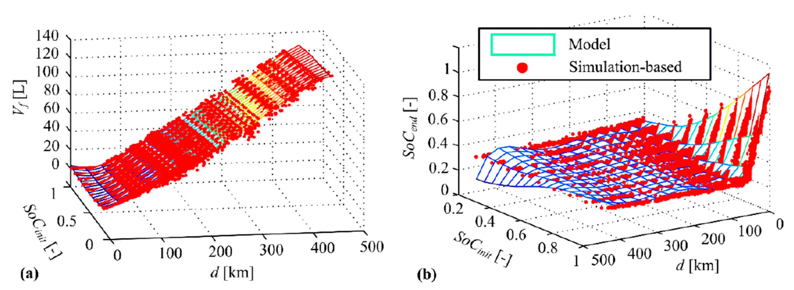
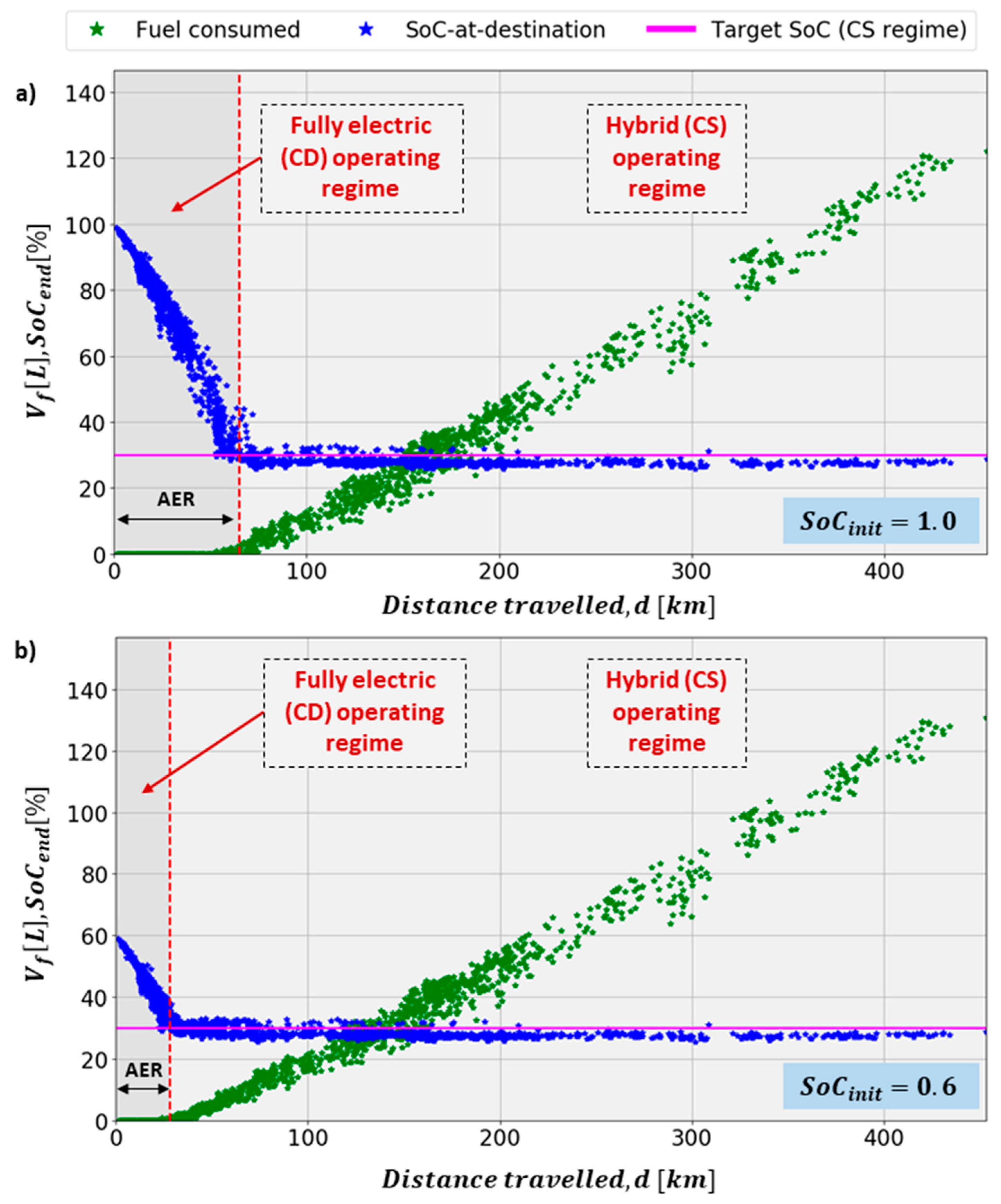
3.2. Simulation Results of Delivery EREV

The delivery EREV model from Figure 5a has been simulated over the full set of 2286 recorded driving cycles for nine discrete levels of initial SoC ($So{C}_{init}\in \left[0.2, 0.3,\dots , 1.0\right]$), in order to obtain the fuel consumption, SoC at destination and AER data aimed to be used for NN training and validation. This resulted in total of 20,574 simulations.

The vehicle mass m_v, which includes both the empty vehicle mass and the cargo mass, is set to 10,066 kg (i.e., empty vehicle mass + average mass for the recorded driving cycles) and is kept constant for all driving cycles. The impact of the road slope α in Equation (1) is neglected (α is set to 0) due to a relatively flat area over which the considered delivery vehicle fleet were operating.

Figure 6 shows the relation of both the simulated fuel consumption V_f and the SoC at destination (i.e., at the end of a driving cycle, SoC_end) with respect to travelled distance d for the case of SoC_init equal to 1.0 (Figure 6a), and for the case of SoC_init equal to 0.6 (Figure 6b). It can be observed from these results that the initial SoC and travelled distance d highly influence the fuel consumption V_f and SoC at destination (i.e., at the given d).

This is the reason why these variables were used as inputs for predicting energy demand when using the response surface modeling approach (see [4] and Section 4 for more details). However, it should be noted that there is notable scattering of both fuel consumption (V_f) and SoC at destination data (SoC_end) for the given distance travelled d, which is caused by variability in driving cycles features (reflecting different driving routes, driving styles and traffic congestion aspects). This means that the fuel consumption, the SoC at destination and also the AER (see Figure 7) cannot be accurately captured solely by using travelled distance and initial SoC inputs.

4. Modeling of Energy Demand

This section first describes the traditional map-based approach (i.e., response surface method) of energy demand modeling, which is based on simulation of the delivery EREV model over synthetic driving cycles (more details are given in [4]). The emphasis is then on NN modeling approach, where the MLP and CNN network architectures are considered.

4.1. Response Surface Modeling Approach

Because both vehicle fuel consumption V_f and SoC-at-destination SoC_end predominantly depend on the initial SoC (SoC_init) and the travelled distance d (see Section 3 and Figure 6), the energy demand model is based on the following functional dependences [4,5]:

$$V_f=f_1\left(So{C}_{init}, d\right),$$

(7)

$$So{C}_{end}=f_2\left(So{C}_{init}, d\right).$$

(8)

The response surface approach is appropriate for this modeling application, because the resulting model is typically computationally very efficient and easy to be parameterized. The modeling procedure includes the following steps [4]: (i) clustering of recorded driving cycles by travelled distance into several groups, (ii) generating and validating single representative synthetic driving cycle for each cluster, (iii) defining levels of initial SoC, (iv) performing simulations of EREV model over each generated synthetic driving cycle for each defined level of initial SoC, (v) forming response surfaces based on the simulation results. Figure 8 shows the obtained response surface model in the form of two-dimensional approximation polynomials (labeled as Model) defined by Equations (7) and (8), along with the simulation results based on recorded driving cycles [4].

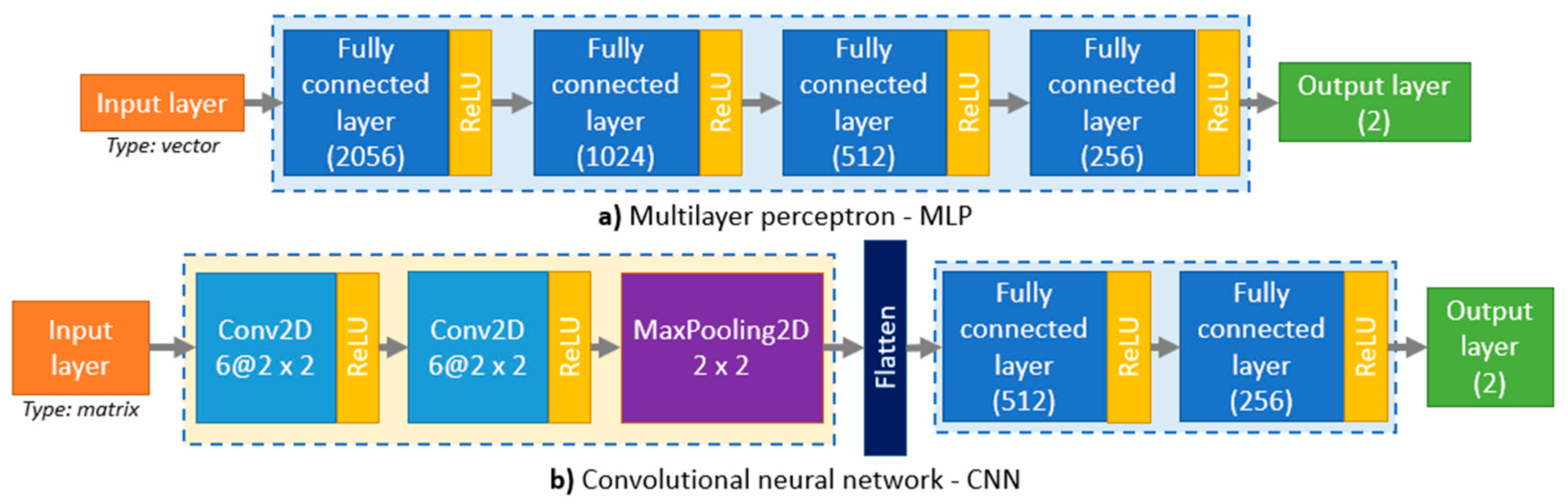
4.2. Neural Network Modeling Approach

4.2.1. Energy Demand Modeling

Using of NNs for energy demand modeling is motivated by the universal approximation theorem for NNs, which states that a feedforward NN with a linear output layer and at least one hidden layer containing a finite number of neurons, can approximate any continuous function of finite dimensional space to any certain target amount of error [33]. Two NN architectures have been considered for the purpose of EV energy demand modeling. The first architecture corresponds to MLP, and consists of a single input layer, four fully connected (i.e., hidden) layers with 2056, 1024, 512, and 256 neurons, respectively, and the single output layer (see Figure 9a). The second NN architecture corresponds to CNN, and consists of a single input layer, two convolutional layers with six convolutional filters of size 2 × 2, one max-pooling layer of size 2 × 2, one flattened layer, two fully connected layers with 512 and 256 neurons, and the single output layer (see Figure 9b). The former one is chosen because it represents standard NN architecture, while the latter one is selected because it has been proven to be very successful in image classification tasks (due to its effectiveness in automatic feature extraction) and the processed driving cycles can be considered as images (i.e., 2D matrices in the case of IT2 and IT3; see Figure 2, Figure 3 and Figure 4).

Both MLP and CNN models take the driving cycle data with incorporated initial SoC value (SoC_init) as inputs (see description of IT1, IT2, and IT3 in Section 2), and they output the predicted fuel consumption (V_f) and SoC at destination (SoC_end) values. The corresponding NN architectures are implemented in Python programming language (version 3.5.0), by using the Keras module [34] with Tensorflow [35] as backend. The stride property (i.e., the number of pixels by which the filter matrix slides over the input matrix) of the considered two-dimensional convolutional and max-pooling layers, represented as Conv2D and MaxPooling2D in Figure 9, is set to 1. The abbreviation ReLU stands for rectifier linear unit, i.e., the non-linear activation function used in developed NN models, which avoids negative values by mapping them to zero, thus allowing the more effective training of the networks. For the purpose of training the developed NNs, Adam (i.e., adaptive moment estimation) optimization algorithm for stochastic gradient descent is used, with its parameters set to default values [36]. The batch size and the number of epochs are set to 32 and 300, respectively. The loss function E to be minimized by training is defined as mean squared error (MSE) between the given NN output y_net and the desired output y_train:

$$\mathit{E}\left(\mathit{X}, \mathit{W}\right)=\frac{1}{2n}{{\displaystyle \sum }}_{i=1}^n{\left({\mathit{y}}_{train,i}-{\mathit{y}}_{net,i}\right)}^2,$$

(9)

where X represents the input vector or matrix, y_net = [V_f SoC_end]^T is the vector of energy demand data obtained by EREV simulation over recorded driving cycles, W are the network weights, and n is the length of the overall training dataset (in this case it equals to 17,488, i.e., 85% of the obtained simulation dataset; see Section 3 for detailed information).

4.2.2. All-Electric Range Modeling

The EREV fleet AER is described by the same CNN model as for predictions of vehicle fuel consumption and SoC at destination (see Figure 9b), but with its output dimension changed to 1 (i.e., model outputs a single value of AER). The AER model uses input of type IT3 to whom the following minor modification were made: (i) each of the matrix rows are normalized with respect to the sum of belonging elements, and (ii) all of the matrix fields are incremented by the corresponding initial SoC values ($So{C}_{init}=\left(0.2, 0.3, \dots ,1.0\right)$). This modification of IT3 were introduced because AER is more dependent on driving style than on the total distance travelled (see Figure 7). More specifically, the normalization of matrix rows effectively converts the information about counted velocity and acceleration states into the transition probabilities between the related states, thus giving more focus on a driving style, while suppressing the information about total distance travelled and resulting in better AER predictions. The opposite applies to the case of V_f and SoC_end modeling, where the distance travelled is the dominant influencing parameter, so that the matrix rows remain in the absolute (non-normalized) form, thus reflecting the distance travelled.

5. Analysis of Modeling Results

This section presents a detailed comparative analysis of the energy demand and AER prediction results obtained by the response surface- and NN-based models. The computations are performed on a HP Z440 Workstation, equipped with 16 GB RAM and an Intel^® Xeon^® Processor E5-1620 v3 @ 3.50 GHz.

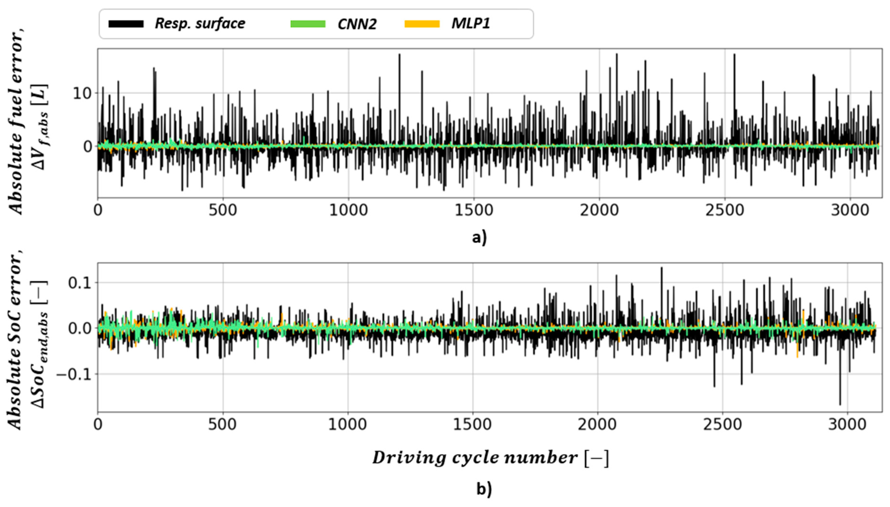
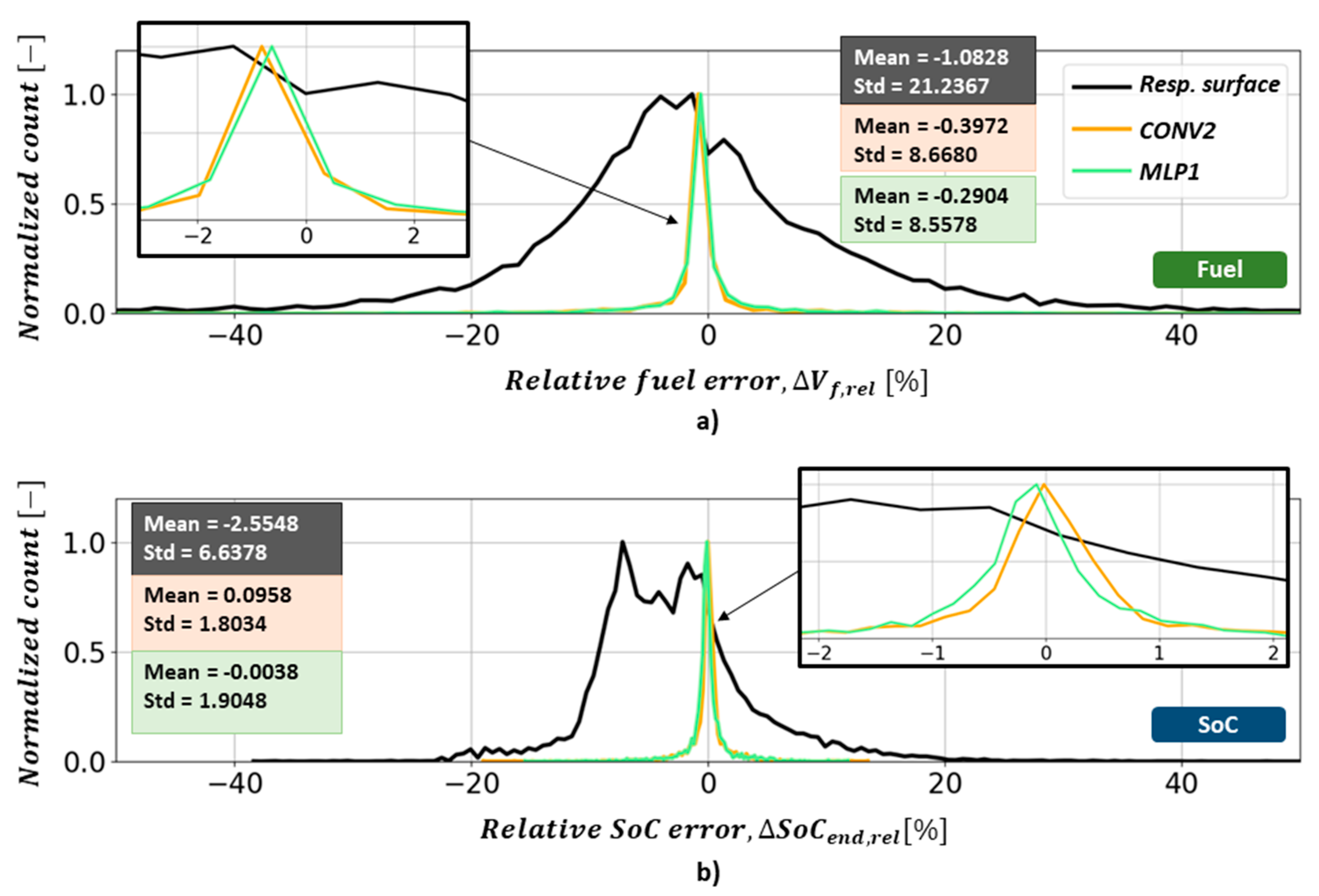
5.1. Energy Demand Prediction

First, the recorded driving cycles have been processed and the inputs of predefined formats obtained (IT1, IT2, and IT3; see Section 2). Next, the response surface- and NN-based models have been derived based on generated EREV simulation-based energy demand data (see Section 4), finally, the derived models have been evaluated over those inputs giving several key performance indicators. The performance indicators related to the response surface-based model reflect basic statistics of the obtained prediction results and related residuals (i.e., difference between model-predicted and reference values), while the NN-based models include some additional indicators such as: (i) training time in hours, (ii) evaluation time in milliseconds, (iii) training score which corresponds to the value of loss function E for the case of training dataset, (iv) testing score which corresponds to the value of loss function E for the case of testing dataset, and (v) the total number of trainable parameters. The basic statistics information considers the minimum (min), maximum (max), mean, median, standard deviation (std), and 95% confidence interval (CFI 95%) of the prediction errors (i.e., residuals; see Equations (10) and (12) given below). The confidence intervals are calculated as $\mathrm{CFI}95\%=\mathrm{mean}\pm 2·\mathrm{std}$ (under the assumption of normal distribution of residuals).

The results related to NN-based models are given for five different cases, concerning two NN architectures and three input formats (MLP for IT1, MLP for IT3, MLP for IT2, CNN for IT2, and CNN for IT3; see

Table 2. Performance measures of NN-based models concerning different NN architectures and input data types.

Model Label	Input Label	Input Dim.	Training Time [h]	Evaluation Time [ms]	Training Score	Testing Score	Trainable Params
MLP1	IT1 *	182	2.596	9.345	0.01329	0.19356	3,139,258
MLP2	IT3 *	5612	17.846	11.128	0.01006	0.49081	14,303,338
MLP3	IT2 *	8282	21.751	10.514	0.00922	0.30432	19,792,858
CNN1	IT2	91 × 91	9.967	4.500	0.05745	0.25890	6,079,926
CNN2	IT3	91 × 31	7.594	3.413	0.00531	0.17379	3,960,246

* Refers to flattened version of the given input type, i.e., vector. Note: Fields marked in green represent the best results.

), and they are compared with the results obtained by using the response surface-based models.

Table 3. Basic statistical indicators of SoC-at-destination (SoC_end) predictions for both response surface- and NN-based energy demand models.

$\mathbf{Performance}\mathbf{of}\mathbf{SoC}\text{-}\mathbf{at}\text{-}\mathbf{Destination}\mathbf{Predictions}[\%]:\Delta \mathit{S}\mathit{o}{\mathit{C}}_{\mathit{e}\mathit{n}\mathit{d}, \mathit{a}\mathit{b}\mathit{s}}=\mathit{S}\mathit{o}{\mathit{C}}_{\mathit{e}\mathit{n}\mathit{d},\mathit{p}\mathit{r}\mathit{e}\mathit{d}\mathit{i}\mathit{c}\mathit{t}}-\mathit{S}\mathit{o}{\mathit{C}}_{\mathit{e}\mathit{n}\mathit{d},\mathit{r}\mathit{e}\mathit{a}\mathit{l}}$
Model Label	Min	Median	Mean	Max	Std	CFI 95%
MLP1	−4.3172	−0.0032	0.0031	3.8625	0.5878	[−1.173, 1.179]
MLP2	−4.2536	−0.0223	0.0412	13.3202	0.9547	[−1.868, 1.950]
MLP3	−4.4600	0.0389	0.0551	10.2145	0.7504	[−1.446, 1.556]
CNN1	−6.0190	−0.0038	−0.0156	5.0332	0.6698	[−1.356, 1.324]
CNN2	−6.4613	0.0498	0.0351	4.3829	0.5602	[−1.085, 1.155]
Resp. surface *	−18.9968	−1.0147	−0.6972	16.5657	2.3197	[−5.337, 3.942]

* Refers to response surface-based energy demand model. Note: Fields marked in green represent the best results.

and

Table 4. Basic statistical indicators of fuel consumption (V_f) predictions for both response surface- and NN-based energy demand models.

$\mathbf{Performance}\mathbf{of}\mathbf{Fuel}\mathbf{Consumption}\mathbf{Predictions}\left[\mathbf{L}\right]:\Delta {\mathit{V}}_{\mathit{f}, \mathit{a}\mathit{b}\mathit{s}}={\mathit{V}}_{\mathit{f},\mathit{p}\mathit{r}\mathit{e}\mathit{d}\mathit{i}\mathit{c}\mathit{t}}-{\mathit{V}}_{\mathit{f},\mathit{r}\mathit{e}\mathit{a}\mathit{l}}$
Model Label	Min	Median	Mean	Max	Std	CFI 95%
MLP1	−1.3655	−0.0138	−0.0147	1.8408	0.2034	[−0.422, 0.392]
MLP2	−1.0489	0.0043	0.0161	3.5083	0.2612	[−0.506, 0.538]
MLP3	−1.2630	0.0307	0.0341	2.7904	0.2035	[−0.373, 0.441]
CNN1	−2.7871	0.0301	0.0259	2.9722	0.2613	[−0.497, 0.549]
CNN2	−1.4150	−0.0099	−0.0076	1.1924	0.1801	[−0.368, 0.352]
Resp. surface *	−8.5247	0.0000	0.0569	17.2393	2.6067	[−5.157, 5.270]

* Refers to response surface-based energy demand model. Note: Fields marked in green represent the best results.

present detailed statistical information of the prediction results (i.e., residual errors) considering the vehicle fuel consumption (V_f) and SoC at destination (SoC_end) for both response surface- and NN-based models. These results point out that CNN2 (CNN in combination with IT3 input, i.e., 2D matrix including velocity and acceleration information) yields best results both in training score and testing score, as well as in evaluation time (the best scores are marked in green color). On the other hand, MLP1 has a significantly shorter training time, which is due to the lower number of trainable parameters resulting from the smaller input dimension. The CNN2 yields overall best results regarding the predictions of fuel consumption V_f and SoC_end, as well, while the MLP1 results follow them very closely. Therefore, graphical plots presented below are given only for these two cases.

Furthermore, in order to gain better insight into precision of the developed NN-based energy demand models when compared to the traditional response surface-based models, the distributions of both fuel consumption and SoC-at-destination prediction errors ∆V_f and ∆SoC_end are analyzed, where two types of prediction errors (i.e., relative: rel, and absolute: abs) are considered:

$$\Delta V_{f, abs}=V_{f,predict}-V_{f,real} \left[L\right],$$

(10)

$$\Delta V_{f,rel}=\frac{V_{f,predict}-V_{f,real}}{V_{f,real}} [\%],$$

(11)

$$\Delta So{C}_{end,abs}=So{C}_{end,predict}-So{C}_{end,real} [-],$$

(12)

$$\Delta So{C}_{end, rel}=\frac{So{C}_{end,predict}-So{C}_{end,real}}{So{C}_{end,real}}[\%],$$

(13)

The fuel- and SoC-related absolute prediction errors ∆V_f,abs and ∆SoC_end,abs are shown in Figure 10, while the distributions of absolute and relative errors calculated according to Equations (10)–(13), along with the corresponding mean values (Mean) and standard deviations (Std), are shown in Figure 11 and Figure 12, respectively. The results shown in Figure 12 indicate that most of the relative prediction errors for both ∆V_f,rel and ∆SoC_end,rel and both MLP1 and CNN2 models are located within the ±2% interval, which are significantly better results when compared to the response surfaces model whose distributions of errors are far wider (i.e., ±20%).

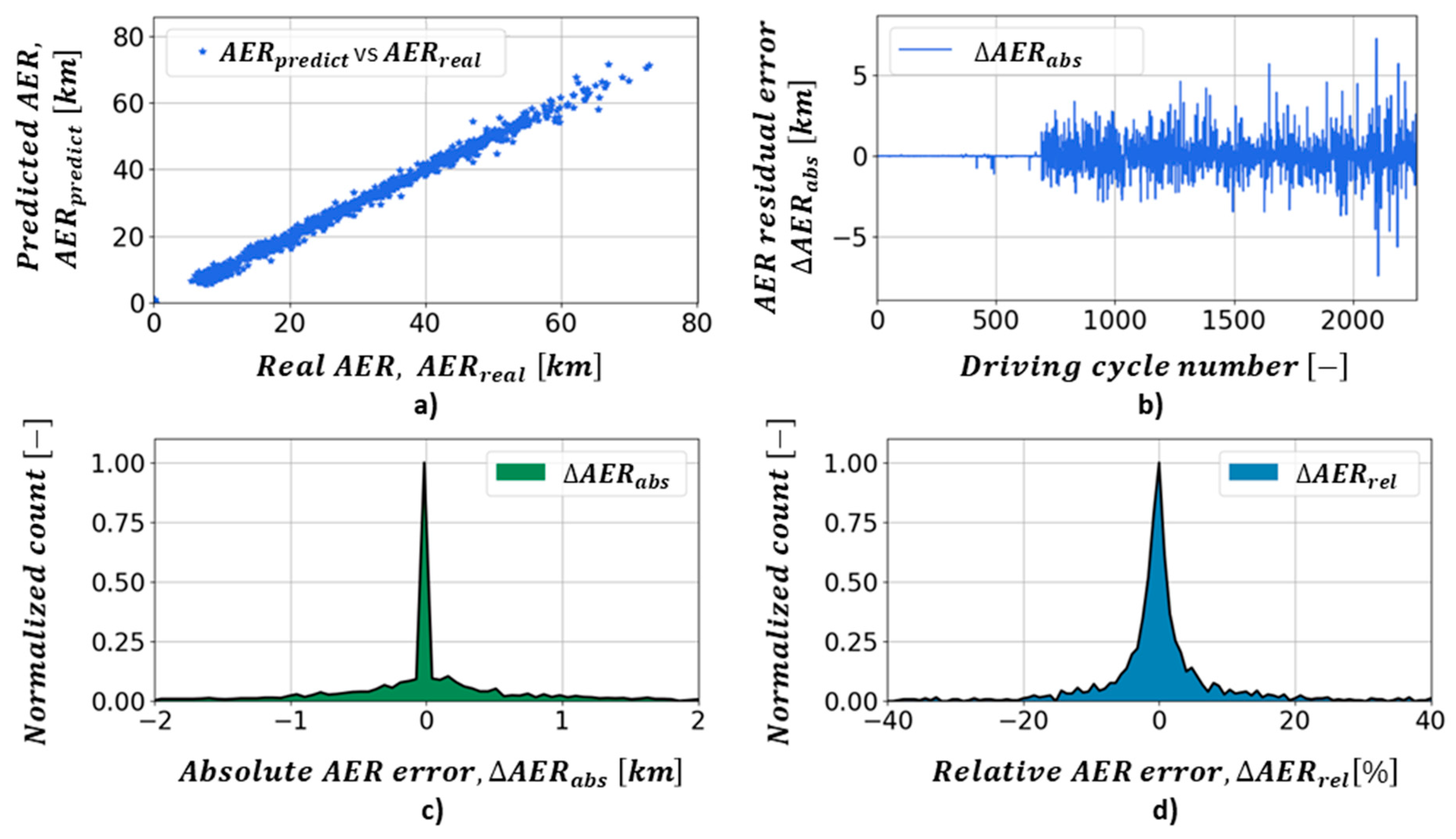
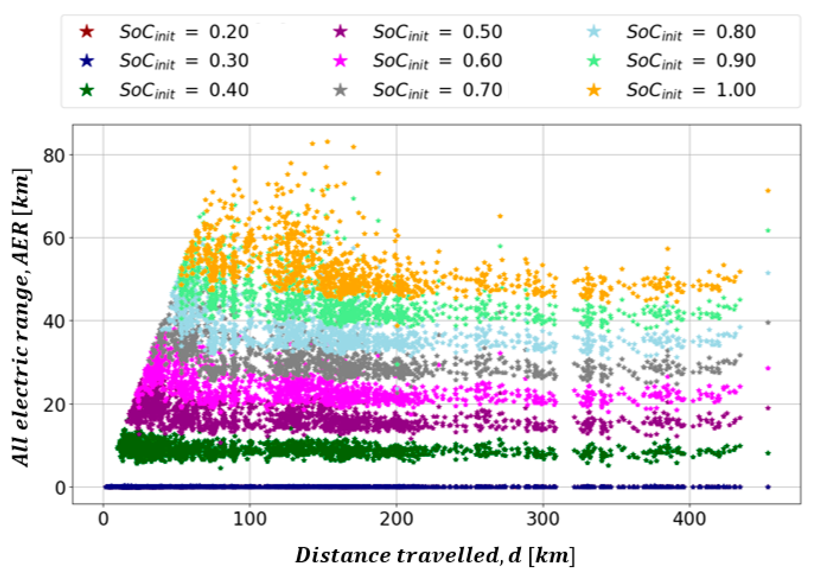
5.2. All-Electric Range (AER) Prediction

The corresponding CNN-based prediction results including the basic statistics of the absolute AER errors calculated as $\Delta AE{R}_{abs}=AE{R}_{predict}-AE{R}_{real}$ are given in

Table 5. Basic statistical indicators of AER predictions for CNN-based model.

$\mathbf{Performance}\mathbf{of}\mathbf{AER}\mathbf{Predictions}\left[\mathbf{km}\right]:\Delta \mathit{A}\mathit{E}{\mathit{R}}_{\mathit{a}\mathit{b}\mathit{s}}=\mathit{A}\mathit{E}{\mathit{R}}_{\mathit{p}\mathit{r}\mathit{e}\mathit{d}\mathit{i}\mathit{c}\mathit{t}}-\mathit{A}\mathit{E}{\mathit{R}}_{\mathit{r}\mathit{e}\mathit{a}\mathit{l}}$
Min	Median	Mean	Max	Std	CFI 95%
−7.40366	0.00096	0.04049	7.25466	0.91674	[−1.793, 1.874]

. Figure 13a shows the plot of predicted AER (AER_predict) vs. real AER (AER_real), while the absolute AER errors ∆AER_abs for a given testing dataset are shown in Figure 13b. The distributions of the AER-related residuals (i.e., $\Delta AE{R}_{abs}$ and $\Delta AE{R}_{rel}=\left(AE{R}_{predict}-AE{R}_{real}\right)/AE{R}_{real}$) are shown in Figure 13c,d. These results show that the developed CNN-based model predicts the vehicle AER with an absolute error $\Delta AE{R}_{abs}$ that is approximately 1 km (i.e., most of the points are located within the ±1 km interval; see Figure 13c). Regarding the relative AER error $\Delta AE{R}_{rel}$, the majority of points lays within the ±5% interval (see Figure 13d), which can be considered quite accurate for this kind of prediction tasks. It is worth noting that the same methodology can be used to predict the driving distance of fully electric vehicle, as well.

6. Discussion

Energy demand modeling of an extended range electric vehicle (EREV) has been presented based on applying deep neural networks (NN). The models are aimed at predicting the EREV fuel consumption V_f, SoC-at-destination SoC_end, and all electric range (AER). Special emphasis was placed on proposing proper methods for preprocessing of driving cycles, in order to prepare them to serve as static 1D or 2D inputs to NNs, while conserving driving cycle features relevant to energy demand modeling. Three driving cycle input type formats have been proposed and analyzed: (i) IT1—1D vector which contains counted discrete vehicle velocity values, (ii) IT2—2D matrix which contains counted transitions between discrete vehicle velocity values/states (acceleration included indirectly), and (iii) IT3—2D matrix which contains counted states where each state represents one combination of discrete vehicle velocity and acceleration (acceleration included directly). Reliable options for including the initial SoC (i.e., the one at the beginning of driving cycle) into the NN input have been suggested (e.g., through adding the initial SoC to each element of 2D matrix in the case of IT2 and IT3). Also, two NN architectures have been considered and analyzed in different combinations with input types: (i) standard multi-layer perceptron (MLP); and (ii) convolutional neural network (CNN). The use of CNN architecture has been motivated by its effectiveness in image classification tasks (i.e., automatic feature extraction characteristics), where images are typically represented with 2D matrices, similarly as it is the case with driving cycles-related NN input herein (i.e., IT2 and IT3). The proposed NNs have been trained and examined based on different portions of large energy demand dataset obtained by simulating a delivery EREV model over a wide set of recorded driving cycles. The traditional response surface energy demand modeling approach has also been considered to quantify improvements which can be achieved by applying newly proposed NN methods.

The comparative analysis of the energy-related prediction results has shown that the CNN in combination with IT3 input (i.e., 2D matrix including velocity and acceleration information; CNN2), provides the best results in terms of the training and testing score (mean squared errors), as well as evaluation time (≈3.4 ms), while the MLP1 resulted in a significantly shorter training time (≈2.6 h vs. ≈7.6 h) due to the significantly lower input dimensions of IT1 when compared to IT3 (vector of dimension 182 vs. matrix of dimension 91 × 31). Furthermore, it is shown that most of the prediction errors (residuals) for both the fuel consumption ∆V_f,rel and the SoC-at-destination ∆SoC_end,rel in cases of MLP1 and CNN2 are located within the ±2% interval, which is significantly better when compared to the response surface model whose distributions of errors are far wider (i.e., most errors lays within the ±20% interval). The CNN-based model has been retrained for the purpose of prediction of vehicle AER. It is shown that the AER predictions are slightly less precise while compared to the energy-related prediction models (i.e., the majority of relative prediction errors ∆AER_,rel lays within the ±5%; or ±1 km in terms of absolute errors ∆AER_,abs), but this can still be considered quite accurate for this kind of prediction task.

7. Conclusions

It can be concluded that NN-based energy demand models are significantly more accurate than response surface models, because response surfaces only include the driving distance d as input, along with the initial SoC; while NNs, apart from the driving distance (contained implicitly within inputs), also include other significant driving cycle features contained within NN inputs through automatic feature extraction. When considering model prediction accuracy, it has been found that the CNN-based energy demand model in combination with IT3 input form is the most successful in this automatic feature extraction. Apart from the high prediction accuracy, NN-based models are shown to be very computationally efficient (e.g., 3.4 ms of evaluation time in the case of CNN and IT3), and can therefore be used in various applications which require real-time performance such as vehicle routing and charging management. In the latter case, the accurate prediction of SoC at destination represents a key input to advanced, predictive charging management strategies, which need to satisfy the required driving missions and minimize the charging energy cost. Future work can consider other vehicle and environment parameters (e.g., vehicle mass and road slope) as inputs to NN for more accurate predictions in general case.

References

1. Suhail Hussain, S.M.; Ustun, T.S.; Nsonga, P.; Ali, I. IEEE 1609 WAVE and IEC 61850 Standard Communication Based Integrated EV Charging Management in Smart Grids. IEEE Trans. Veh. Technol. 2018, 67, 7690–7697. [Google Scholar] [CrossRef]
2. De Cauwer, C.; Verbeke, W.; Coosemans, T.; Faid, S.; Van Mierlo, J. A Data-Driven Method for Energy Consumption Prediction and Energy-Efficient Routing of Electric Vehicles in Real-World Conditions. Energies 2017, 10, 608. [Google Scholar] [CrossRef]
3. Nageshrao, S.P.; Jacob, J.; Wilkins, S. Charging cost optimization for EV buses using neural network based energy predictor. IFAC-Pap. 2017, 50, 5947–5952. [Google Scholar] [CrossRef]
4. Škugor, B.; Deur, J. Synthetic Driving Cycles-based Modelling of Extended Range Electric Vehicle Fleet Energy Demand. In Proceedings of the 30th International Electric Vehicle Symposium & Exhibition, Stuttgart, Germany, 9–11 October 2017. [Google Scholar]
5. Lee, T.K.; Filipi, Z.S. Response surface modelling approach for the assessment of the PHEV impact on the grid. In Proceedings of the IEEE Vehicle Power and Propulsion Conference, Chicago, IL, USA, 6–9 September 2011. [Google Scholar]
6. Škugor, B.; Deur, J. Delivery vehicle fleet data collection, analysis, and naturalistic driving cycle synthesis. Int. J. Innov. Sustain. Dev. 2016, 10, 19–33. [Google Scholar] [CrossRef]
7. Lee, T.K.; Filipi, Z.S. Synthesis of real-world driving cycles using stochastic process and statistical methodology. Int. J. Veh. Des. 2011, 56, 43–62. [Google Scholar] [CrossRef]
8. Brand, C.; Anable, J.; Morton, C. Lifestyle, efficiency and limits: Modelling transport energy and emissions using a socio-technical approach. Energy Effic. 2019, 12, 187–207. [Google Scholar] [CrossRef]
9. Geem, Z.W. Transport energy demand modeling of South Korea using artificial neural network. Energy Policy 2011, 39, 4644–4650. [Google Scholar] [CrossRef]
10. Murat, Y.S.; Halim, C. Use of artificial neural networks for transport energy demand modelling. Energy Policy 2006, 34, 3165–3172. [Google Scholar] [CrossRef]
11. Teng, G.; Xiao, J.; He, Y.; Zheng, T.; He, C. Use of group method of data handling for transport energy demand modelling. Energy Sci. Eng. 2017, 5, 302–317. [Google Scholar] [CrossRef]
12. Shankar, R.; Marco, J. Method for estimating the energy consumption of electric vehicles and plug-in hybrid electric vehicles under real-world driving conditions. IET Intell. Transp. Syst. 2013, 7, 138–150. [Google Scholar] [CrossRef]
13. Zeng, T.; Zhang, C.; Hu, M.; Chen, Y.; Yuan, C.; Chen, J.; Zhou, A. Modelling and predicting energy consumption of a range extender fuel cell hybrid vehicle. Energy 2018, 165, 187–197. [Google Scholar] [CrossRef]
14. Delogu, M.; Del Pero, F.; Pierini, M. Lightweight Design Solutions in the Automotive Field: Environmental Modelling Based on Fuel Reduction Value Applied to Diesel Turbocharged Vehicles. Sustainability 2016, 8, 1167. [Google Scholar] [CrossRef]
15. Zeiler, M.D.; Fergus, R. Visualizing and Understanding Convolutional Neural Networks. In Proceedings of the 13th European Conference on Computer Vision, Zurich, Switzerland, 6–12 September 2014; pp. 818–833. [Google Scholar]
16. Szegedy, C.; Liu, W.; Jia, Y.; Sermanet, P.; Reed, S.; Anguelov, D.; Erhan, D.; Vanhoucke, V.; Rabinovich, A. Going Deeper with Convolutions. In Proceedings of the IEEE Conference on Computer Vision and Pattern Recognition, Boston, MA, USA, 7–12 June 2015. [Google Scholar]
17. A Medium Corporation. Available online: https://medium.com/@siddharthdas_32104/cnns-architectures-lenet-alexnet-vgg-googlenet-resnet-and-more-666091488df5 (accessed on 21 May 2018).
18. Tian, Y.; Pei, K.; Jana, S.; Ray, B. DeepTest: Automated Testing of Deep-Neural-Network-driven Autonomous Cars. In Proceedings of the 40th International Conference on Software Engineering, Gothenburg, Sweden, 27 May–3 June 2018; pp. 303–314. [Google Scholar]
19. Chen, C.; Seff, A.; Kornhauser, A.; Xiao, J. DeepDriving: Learning affordance for direct perception in autonomous driving. In Proceedings of the 15th IEEE International Conference on Computer Vision, Santiago, Chile, 11–18 December 2015. [Google Scholar]
20. Lemieux, J.; Ma, Y. Vehicle Speed Prediction Using Deep Learning. In Proceedings of the 2015 IEEE Vehicle Power and Propulsion Conference, Montreal, QC, Canada, 19–22 October 2015. [Google Scholar]
21. Jia, Y.; Wu, J.; Du, Y. Traffic speed prediction using deep learning method. In Proceedings of the 2016 IEEE 19th International Conference on Intelligent Transportation Systems, Rio de Janeiro, Brazil, 1–4 November 2016; pp. 1217–1222. [Google Scholar]
22. Song, C.; Lee, H.; Kang, C.; Lee, W.; Kim, Y.B.; Cha, S.W. Traffic speed prediction under weekday using convolutional neural networks concepts. In Proceedings of the 2017 IEEE Intelligent Vehicles Symposium, Redondo Beach, CA, USA, 11–14 June 2017; pp. 1293–1298. [Google Scholar]
23. Park, J.; Chen, Z.; Kiliaris, L.; Kuang, M.L.; Masrur, M.A.; Phillips, A.M.; Murphey, Y.L. Intelligent vehicle power control based on machine learning of optimal control parameters and prediction of road type and traffic congestion. IEEE Trans. Veh. Technol. 2009, 58, 4741–4756. [Google Scholar] [CrossRef]
24. Zhang, X.; Chan, K.W.; Yang, X.; Zhou, Y.; Ye, K.; Wang, G. A comparison study on electric vehicle growth forecasting based on grey system theory and NAR neural network. In Proceedings of the 2016 IEEE International Conference on Smart Grid Communications, Sydney, Australia, 6–9 November 2016. [Google Scholar]
25. He, H.; Yan, M.; Sun, C.; Peng, J.; Li, M.; Jia, H. Predictive air-conditioner control for electric buses with passenger amount variation forecast. Appl. Energy 2018, 227, 249–261. [Google Scholar] [CrossRef]
26. Lopez, K.L.; Gagne, C.; Gardner, M. Demand-Side Management using Deep Learning for Smart Charging of Electric Vehicles. IEEE Trans. Smart Grid 2018. [Google Scholar] [CrossRef]
27. Morsalin, S.; Mahmud, K.; Town, G. Electric vehicle charge scheduling using an artificial neural network. In Proceedings of the 2016 IEEE Innovative Smart Grid Technologies—Asia, Melbourne, VIC, Australia, 28 November–1 December 2016. [Google Scholar]
28. Zhou, F.; Wang, L.; Lin, H.; Lv, Z. High accuracy state-of-charge online estimation of EV/HEV lithium batteries based on Adaptive Wavelet Neural Network. In Proceedings of the 2013 IEEE ECCE Asia Downunder, Melbourne, Australia, 3–6 June 2013. [Google Scholar]
29. Tian, H.; Ouyang, B. Estimation of EV battery SOC based on KF dynamic neural network with GA. In Proceedings of the 2018 Chinese Control and Decision Conference, Shenyang, China, 9–11 June 2018. [Google Scholar]
30. Affanni, A.; Bellini, A.; Concari, C.; Franceschini, G.; Lorenzani, E.; Tassoni, C. EV battery state of charge: Neural network based estimation. In Proceedings of the IEEE International Electric Machines and Drives Conference, Madison, WI, USA, 1–4 June 2013. [Google Scholar]
31. Cipek, M.; Škugor, B.; Deur, J. Comparative Analysis of Conventional and Electric Delivery Vehicles Based on Realistic Driving Cycles. In Proceedings of the European Electric Vehicle Congress, Brussels, Belgium, 2–5 December 2014. [Google Scholar]
32. Škugor, B.; Cipek, M.; Deur, J. Control Variables Optimization and Feedback Control Strategy Design for the Blended Operating Regime of an Extended Range Electric Vehicle. SAE Int. J. Altern. Powertrains 2014, 3, 52–162. [Google Scholar] [CrossRef]
33. Goodfellow, I.; Bengio, Y.; Courville, A. Deep Learning; MIT Press: Cambridge, MA, USA, 2016; pp. 198–201. [Google Scholar]
34. Keras. Available online: https://keras.io (accessed on 22 May 2018).
35. Tensorflow. Available online: https://www.tensorflow.org (accessed on 22 May 2018).
36. Kingma, D.P.; Ba, J. Adam: A method for stochastic optimisation. In Proceedings of the 3rd International Conference for Learning Representations, San Diego, CA, USA, 7–9 May 2015. [Google Scholar]
Figure 1. Illustration of the vehicle energy demand modeling procedure including definition of NN input type formats (i.e., IT1, IT2, IT3) and NN architectures (i.e., MLP, CNN).
Energies 12 01396 g001
Figure 2. Illustration of process of generating NN input type IT2.
Energies 12 01396 g002
Figure 3. Illustration of process of generating NN input type IT3.
Energies 12 01396 g003
Figure 4. Contour plots of IT2 and IT3 input matrices for initial SoC values equal to 0%, 30% and 60%.
Energies 12 01396 g004
Figure 5. Block diagram of the backward-looking model of EREV truck powertrain (a), and equivalent battery circuit (b) [4].
Energies 12 01396 g005
Figure 6. EREV fuel consumptions ( V f ) and SoC at destination ( S o C e n d ) in dependence of total distance travelled ( d ) for cases of initial SoC values S o C i n i t = 1.0 (a), and S o C i n i t = 0.6 (b).
Energies 12 01396 g006
Figure 7. EREV all-electric range (AER) in dependence of trip length ( d ) for various initial SoC values ( S o C i n i t ).
Energies 12 01396 g007
Figure 8. Illustration of response surface-based energy demand model for delivery EREV: fuel consumption V f = f 1 ( S o C i n i t ,   d ) (a), and SoC at destination S o C e n d = f 2 ( S o C i n i t ,   d ) (b) [4].
Energies 12 01396 g008
Figure 9. Block diagram of considered neural network architectures: multilayer perceptron—MLP (a), and convolutional neural network—CNN (b); The expression 6 @ 2 × 2 considers the depth of 6 (i.e., the number of convolutional filters in the given Feature Map), where the size of each filter corresponds to 2 × 2 pixels.
Energies 12 01396 g009
Figure 10. Residuals of predicted fuel consumptions ∆Vf,abs (a) and SoC-at-destination ∆SoCend,abs (b) for all driving cycles from the NN testing input dataset.
Energies 12 01396 g010
Figure 11. Distribution of normalized absolute residuals of predicted fuel consumptions ∆Vf,abs (a) and SoC-at-destinations ∆SoCend,abs (b).
Energies 12 01396 g011
Figure 12. Distribution of normalized relative residuals of predicted fuel consumptions ∆Vf,rel (a) and SoC-at-destinations ∆SoCend,rel (b).
Energies 12 01396 g012
Figure 13. Predicted A E R p r e d i c t vs. real A E R r e a l values (a), absolute AER residuals ∆AERabs for given testing input dataset (b), and distributions of absolute (c) and relative (d) predicted AER residuals.
Energies 12 01396 g013