A New Machine-Learning Prediction Model for Slope Deformation of an Open-Pit Mine: An Evaluation of Field Data

Abstract

Effective monitoring of the slope deformation of an open-pit mine is essential for preventing catastrophic collapses. It is a challenging task to accurately predict slope deformation. To this end, this article proposed a new machine-learning method for slope deformation prediction. Ground-based interferometric radar (GB-SAR) was employed to collect the slope deformation data from an open-pit mine. Then, an ensemble learner, which aggregated a set of weaker learners, was proposed to mine the GB-SAR field data, delivering a slope deformation prediction model. The evaluation of the field data acquired from the Anjialing open-pit mine demonstrates that the proposed slope deformation model was able to precisely predict the slope deformation of the monitored mine. The prediction accuracy of the super learner was superior to those of all the independent weaker learners.

1. Introduction

The open-pit mine is a popular mining type in the mining/coal industry [1]. A large-sized open-pit mine can produce a coal seam of 200 m in depth. According to this huge production capacity, open-pit mines provide important coal production and contribute greatly to a country’s economy. However, mining disasters have frequently occurred during the past few decades, such as collapse, landslides, and debris flow [2]. As a result, the stability of a mine’s slope is crucial for safety management. However, when a major deformation occurs, it is often too late to implement effective evacuation and prevention measures. Hence, it is imperative to accurately predict slope deformation before a major deformation [3].

As is well known, the deformation of mine ground is the earliest and most obvious characteristic of a mine disaster [4]. Monitoring technologies, such as global position system (GPS), measuring robot, laser scanner, and ground-based interferometric radar (GB-SAR) are widely used in slope deformation monitoring [5]. Among these technologies, GB-SAR is a relatively new technique to monitor the deformation of open-pit mine side slopes with the features of high precision, gigantic scale, long distance, and non-contact [6]. Dick et al. [4] presented an early warning time-of-failure (TOF) analysis procedure for real-time GB-SAR monitoring in an open-pit mine’s trigger action response plan (TARP). Carlà et al. [5] proposed a method of ground-based satellite interferometry to reduce the uncertainties inherent to the identification and characterization of impending catastrophic slope failures. Nie et al. [6] proposed a medium–short term prediction method based on polynomial (MsTPLP) model for landslide monitoring in the West open-pit mine in Fushun, China. Although many works have been conducted on ground-based SAR and satellite SAR remote sensing systems, no studies have conducted systematic research on deformation prediction based on the information fusion of various deformation factors [7]. To the best of our knowledge, information fusion is essential for establishing an effective deformation prediction model using GB-SAR, while artificial intelligence is a promising tool to provide the information fusion [8,9,10].

The slope deformation is a complex process, and the factors influencing rapid and short-term deformations of open-pit slopes mainly include topographic and geomorphic factors, meteorological factors, and groundwater factors [11]. GB-SAR is able to collect the slope shape coefficient, deformation rate, reverse deformation rate, deformation amplitude, rainfall, temperature, atmospheric pressure, relative humidity, wind speed, and direction. Due to the strong coupling effect of these factors, it is difficult to use traditional regression methods, such as linear regression, to establish accurate deformation estimation models [12]. Artificial intelligence methods, such as artificial neural network (ANN), generalized regression neural network (GRNN), support vector machine (SVM), and extreme learning machine (ELM), have been proven effective in dealing with multi-variate nonlinear prediction problems [13]. Owing to strong learning, fitting, fault tolerance, and anti-interference abilities, these artificial intelligence methods are able to discover distinct connections between geographical, climatic, and hydrographic parameters for slope deformation prediction. Chen and Zeng [14] proposed an improved backpropagation neural network (BPNN) to predict landslide deformation using a case study of the Three Gorges reservoir. Du et al. [15] presented a SVM prediction model for slope surface deformation. Chen et al. [16] presented a regression neural network model for landslide deformation forecasting using multi-sensory measurements. He et al. [17] employed a grey model to predict rock slope deformation. Liu et al. [18] developed a sequential intelligent computing model to forecast slope deformation. Hu et al. [19] used a machine-learning method to model slope deformation as a Gaussian Process. Du et al. [20] established an ELM model for slope deformation estimation. Liu et al. [21] proposed a neuron-fuzzy model for slope deformation estimation. Theoretically, a specific prediction algorithm may be only effective for a certain object; once the research object changes, the prediction performance may degrade dramatically [22]. It is reasonable to aggregate a set of different prediction algorithms into a unified framework to improve the robustness and generalizability of the prediction model, such that the predicted model is adaptive to the changes of object or operation parameters. A recent publication [23] demonstrated that the ensemble learning method is able to aggregate a set of prediction algorithms to enhance prediction accuracy and robustness. Ensemble learning can outperform any single algorithm in the ensemble in terms of prediction accuracy. However, ensemble learning has not been found in slope deformation forecasting. Because of the strong complexity of the nature of the slope deformation process, it is difficult to handle changes of slope parameters with a single prediction algorithm. As a result, it is worth developing an ensemble learning model to improve the prediction accuracy and robustness of slope deformation analysis.

In order to fill the research gap in slope deformation prediction, this article proposes a new ensemble learning model. Five popular artificial intelligence algorithms were adopted into the ensemble framework. Monitoring datasets acquired from the Pingshuo Anjialing open-pit mine were used to evaluate the proposed ensemble learning prediction model. GB-SAR was used to collect the field datasets regarding the geographical, climatic, and hydrographic parameters of the open-pit mine slope. The prediction results demonstrate that the proposed ensemble learning method was able to accurately estimate the slope deformation of the Anjialing open-pit mine.

The rest of this article is organized as follows. The proposed ensemble learning method is described in Section 2, followed by an introduction to data acquisition in the Anjialing open-pit mine in Section 3. The predictive capability of the ensemble learning model is evaluated in Section 4. Concluding remarks are presented in Section 5.

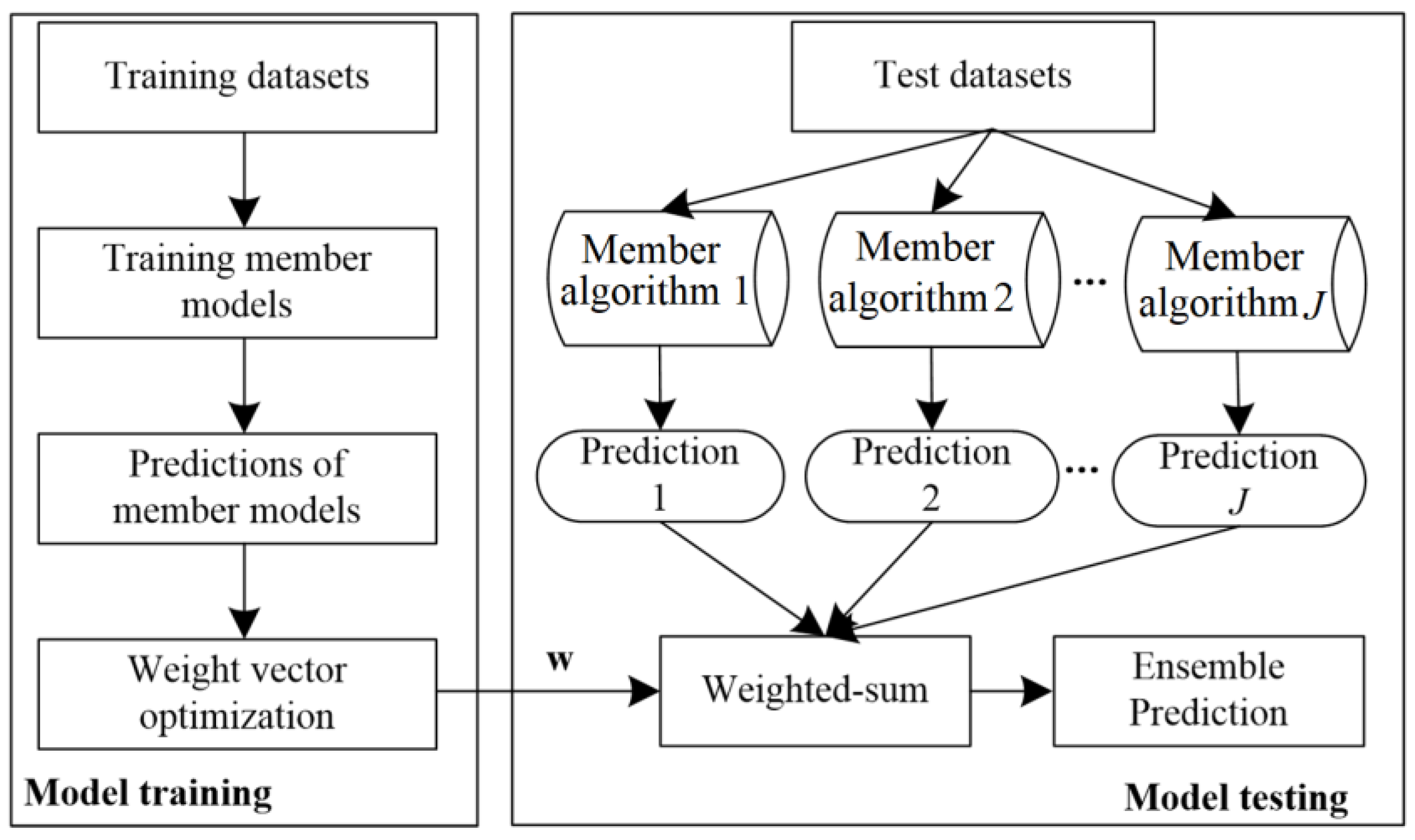
2. The Proposed Method

In this article, the proposed ensemble method was applied to the monitoring of Anjialing open-pit mine. The slope of Anjialing presents characteristics, such as small scale, creep slip, shallow slip, and soil landslide. Hence, the slope deformation type in Anjialing is surface deformation, which is formed by artificial excavation.

Ensemble learning is able to directly use existing algorithm resources to build up an ensemble prognostics method. A weight vector is assigned to each algorithm member, and the weighted sum of all the algorithms outputs the ensemble prognostics result. A nonlinear optimization method is used to optimize the weight vector given a cost function that minimizes the prediction error of the ensemble learning model. Figure 1 shows the flowchart of the proposed ensemble learning method, while

Table 1. A generic computational framework.

Input:	Slope Deformation Datasets
1.	Model training: Calculate the optimal weight vector for member algorithms
1.1	Select appropriate sensory measurements from the ground-based interferometric radar (GB-SAR)
1.2	Train each of the member algorithms to build J member prediction models
1.3	Perform model validation to obtain the predicted deformation of each member model
1.4	Compute the optimal weight vector using nonlinear optimization
2.	Model testing: Perform predictions using ensemble learning
2.1	Predict the slop deformation of the online testing unit using each base learner
2.2	Carry out ensemble prognostics using the optimal weight vector
Output:	Predicted deformation amount

describes the implementation of the ensemble model. In Figure 1, J is the number of member algorithms and w is the weight vector. The generality of the proposed model is that one can select J suitable member algorithms for different prediction problems. Inspired by our literature review, in this article, five popular artificial intelligence algorithms (J = 5) were adopted as the algorithm members in the proposed ensemble learning model, including BPNN, SVM, recurrent neural network (RNN), adaptive network-based fuzzy inference system (ANFIS), and relevant vector machine (RVM).

The sequential quadratic optimization (SQP) [23] procedure was performed to assign a weight value to each member model. The optimization objective was to minimize the prediction error $\epsilon$ of the weighted sum of the predicted deformation $\widehat{D} (={[{\widehat{D}}^1,{\widehat{D}}^2,\dots , {\widehat{D}}^J]}^{\mathrm{T}})$ in the model validation.

$$\{\begin{array}{c}\underset{w}{\mathrm{argmin}}\epsilon =\frac{1}{N}{\displaystyle \sum }f\left(w^{\mathrm{T}}\widehat{D},{\widehat{D}}^T\right)\\ \mathrm{Subject} \mathrm{to} {{\displaystyle \sum }}_{j=1}^J{w}_j=1\end{array}$$

(1)

where w (= [w₁, w₂, …, w_J]^T) is the weight vector and f(•) is a predefined error criterion, such as root-mean-squared error (RSME). The optimal weight vector w^o (= [w₁, w₂, …, w_J]^T) was used for model testing. Then, an ensemble prediction was calculated using the weighted-sum formulation in Equation (2). It is expected that the resulting optimal weight vector will appropriately combine the five member models to enhance the deformation prediction accuracy and robustness.

$${\widehat{D}}_t^P={\displaystyle \sum }_{j=1}^J{w}_j{\widehat{D}}_t^j\left(x_t,X\right)$$

(2)

where x_t is a test dataset; ${\widehat{D}}_t^P$ is the ensemble prediction for x_t; w_j (j = 1, 2, …, J) is the weight assigned to the jth member model; and ${\widehat{D}}_t^j$(x_t, X) denotes the prediction of x_t by the jth member model trained by the training datasets X.

The member algorithms are briefly introduced below. Because BPNN and SVM are discussed in great depth in the literature, we do not describe these two algorithms in this article.

2.1. Relevance Vector Machine

RVM is a Bayesian inference-based learning algorithm [24]. RVM makes predictions based on the following function:

$$\tilde{y}\left(x\right)={{\displaystyle \sum }}_{i=1}^N{\omega }_i\phi \left(x,{\mathbf{x}}_i\right)+{\omega }_0$$

(3)

where $\tilde{y}$ denotes the mapping that estimates the responses from the observations. φ (x, x_i) is a kernel function (e.g., Gaussian kernel) centered at the training point x_i, ω = (ω₀, …, ω_N)^T~$\mathcal{N}$(0, σ⁻¹I) is the weight vector, and σ is the variance of the prior on ω. The likelihood function of the complete dataset can be written as follows:

$$p\left(y|\omega ,{\sigma }^2\right)={\left(2\pi {\sigma }^2\right)}^{-P/2}\exp (-\frac{1}{2{\sigma }^2}\Vert y-\Phi {\omega \Vert }^2)$$

(4)

where Φ is a kernel matrix with dimensions of N × (N + 1) and Φ_ij = φ (x_i, x_j). The Bayesian inference is then applied to Equation (4) to approximate the weight vector ω.

$$p\left(\omega |\gamma \right)={\displaystyle \prod }_{i=0}^N\mathcal{N}\left({\mathsf{\omega }}_i|0,{\gamma }_i^{-1}\right)$$

(5)

where γ = (γ₀, …, γ_N)^T denotes a set of hyperparameters. To specify the Bayesian model, γ and σ² are usually assumed to be subject to the Gamma prior distributions.

$$\{\begin{array}{c}p\left(\mathsf{\gamma }\right)={\displaystyle {\displaystyle \prod }_{i=0}^N}\mathrm{Gamma}\left({\gamma }_i|a,b\right)\hfill \\ p\left({\sigma }^2\right)=\mathrm{Gamma}\left({\sigma }^2|c,d\right)\hfill \end{array}$$

(6)

where $\mathrm{Gamma}\left(\mathsf{\gamma }|a,b\right)=\mathrm{G}{(\mathsf{\gamma })}^{-1}{b}^a{\gamma }^{a-1}{e}^{-b\gamma }$ and G(γ) denotes the gamma function; hyperparameters a, b, c, and d are small constants to ensure a flat Gamma prior in Equation (6). Hence, the posterior probabilities over ω can be estimated by

$$p\left(\omega |y,\gamma ,{\sigma }^2\right)={\left(2\pi \right)}^{-\left(N+1\right)/2}{\left|\Sigma \right|}^{-1/2}\exp (-\frac{1}{2}{\left(\omega -\theta \right)}^T{\Sigma }^{-1}\left(\omega -\theta \right))$$

(7)

where θ (= σ⁻²ΣΦ$\tilde{\mathbf{y}}$) is the mean of the posterior over the weight vector, Σ = (σ⁻²Φ^TΦ+Λ)⁻¹, and Λ = diag(γ). Thus, the expectation maximization (EM) or other iterative optimization algorithms can be applied to the Bayesian model to obtain the optimal hyperparameters γ_p and σ²_p. The distribution of $\tilde{y}$ can be calculated using the optimal values. In this study, the MATLAB program developed by Tipping [24] was employed to build the RVM predictive model. The EM algorithm was used to update the Bayesian model. The Gaussian kernel function with a basis width of 0.5 and a prior variance of σ = 0.2 were used in the RVM model.

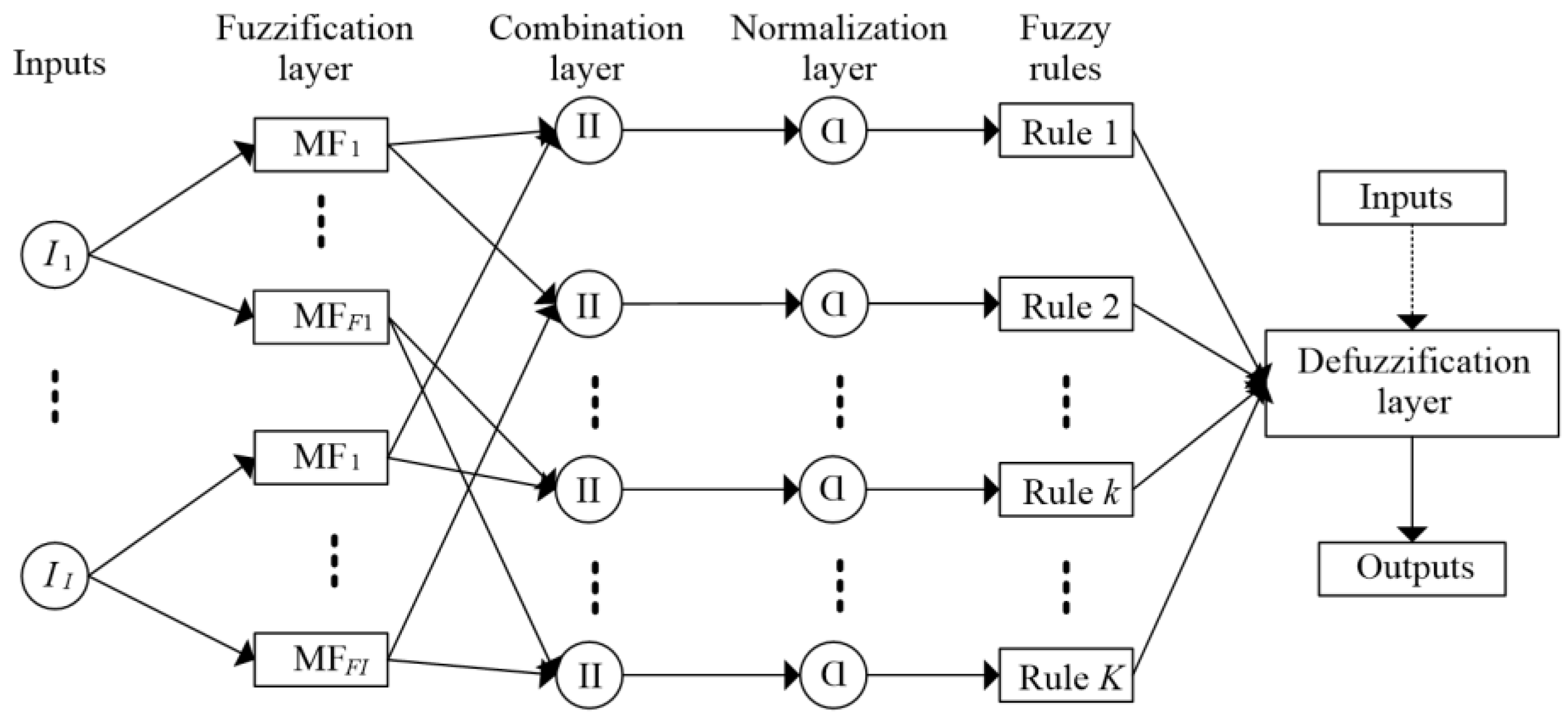
2.2. Adaptive Network-Based Fuzzy Inference System

An adaptive network-based fuzzy inference system (ANFIS) is a technique based on a Takagi–Sugeno fuzzy inference system [25]. Generally, a set of fuzzy if–then rules (usually type-3 rules) is integrated with an ANN to learn the hidden patterns in a training dataset. Figure 2 illustrates a typical architecture of an ANFIS with four layers. Given the inputs I = [I₁, I₂, …, I_I], the first layer fuzzifies the inputs into membership values.

$$O_k^1={\mu }_{ij}\left(I_i\right)$$

(8)

where μ ($·$) denotes a membership function (MF) and O¹ denotes the output of layer 1, the subscript ij denotes the jth membership function of ith input variable, i (= 1, 2,…, I), and j (= 1, 2,…, F_i) with F_i being the membership function numbers of ith input variable. The membership function includes a triangular, bell, or Gaussian function. The parameters in the membership function are called premise parameters.

Layer 2 combines the membership values (i.e., T-norm operator) to obtain the firing strength of each fuzzy rule.

$$O_k^2={\displaystyle \prod }\mu \left(I_k\right)$$

(9)

where O² denotes the output of layer 2, subscript k (= 1, 2,…, K) corresponds to the kth fuzzy rule, K is the total number of rules, and ∏μ(I_k) only involves the membership values of those inputs that contribute the kth fuzzy rule. Layer 3 takes the normalization operator to the firing strength. The output of layer 3 (O³) for the kth rule is described by Equation (10).

$$O_k^3=O_k^2/{\displaystyle \sum }_{k=1}^K{O}_k^2$$

(10)

Layer 4 conducts the defuzzification to produce the real value of each rule.

$$O_k^4=O_k^3\left(A_{k}I+B_k\right)$$

(11)

where O⁴_k denotes the output of kth fuzzy rule, A = [A₁, A₁,…, A_K]^T and B = [B₁, B ₁,…, B _K]^T are the consequent parameters for the Takagi–Sugeno fuzzy model. The sum of O⁴ will give the output of the ANFIS. In this study, the Gaussian function was used as the membership function for the input variables, and each variable had 12 memberships. The fuzzy rule k was 10 in the ANFIS model.

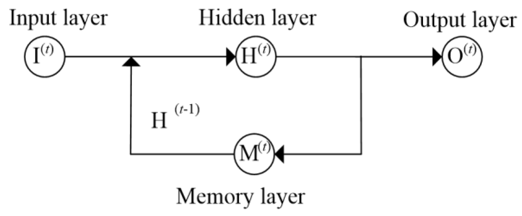
2.3. Recurrent Neural Network

A recurrent neural network is a class of artificial neural networks in which connections between units form a directed cycle [26]. Traditional ANNs, such as radial basis function (RBF) networks and backpropagation networks do not consider the connection of inputs. As opposed to traditional ANNs, a RNN takes the dependence of all inputs into account and makes predictions based on both current and previous inputs. This is achieved by a recurrent mechanism in the hidden layer [26]. Figure 3 illustrates a typical architecture of a RNN consisting of one input layer, one hidden (recurrent) layer with recurrent neural nodes, one memory layer, and one output layer. Given time t, the inputs I^(t) = [I^(t)₁, I^(t)₂, …, I^(t)_I] (I is the neural node number in the input layer), and the previous hidden state H^(t−1) = [H^(t−1)₁, H^(t−1)₂, …, H^(t1)_H] (H is the number of neural nodes in the hidden layer) are connected to the hidden layer by the weights W^HI and W^HM, respectively. The current hidden state H^(t) = [H^(t)₁, H^(t)₂, …, H^(t)_H] is calculated by

$$H^{\left(t\right)}=g\left(W^{HI}{I}^{\left(t\right)}+W^{HM}{H}^{\left(t-1\right)}\right)$$

(12)

where g ($·$) is an activation function. The sigmoid function was used in this work, namely g (x) = (1 + e^−x)⁻¹. The hidden layer H^(t) is connected to the output layer O^(t) = [O^(t)₁, O^(t)₂, …, O^(t)_O] (O is the neural node number in the output layer) by the weights W^OH.

$$O^{\left(t\right)}=f\left(W^{OH}{H}^{\left(t\right)}\right)$$

(13)

As shown in Figure 3, the memory layer holds the previous hidden state H^(t−1) by feeding back the current activities of neural nodes through the recurrent weights W^HM, and hence, the output H^(t) is the contribution of current and previous hidden states. The connections between the inputs at different timesteps can be included in the prediction behavior of the network. In this study, the MATLAB program developed by Cernansky [26] was used to establish the RNN predictive model, in which the number of nodes in the hidden layer was 10 and the output node number was 1.

3. Field Data

In this work, field datasets acquired from the Anjialing open-pit mine in Pingshuo, China, were used to evaluate the proposed ensemble model for predicting the slope deformation. The Anjialing open-pit mine is one of the oldest and largest open-pit mines in China, and its capacity is 30 million tons per year. The type of coal produced in this region is mainly gas coal with an average thickness of 30 m and a depth between 100 and 200 m. According to this huge production capacity, the Anjialing open-pit mine is one of the most important coal energy production bases in China.

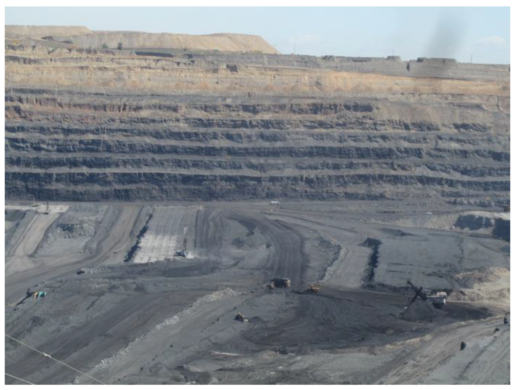
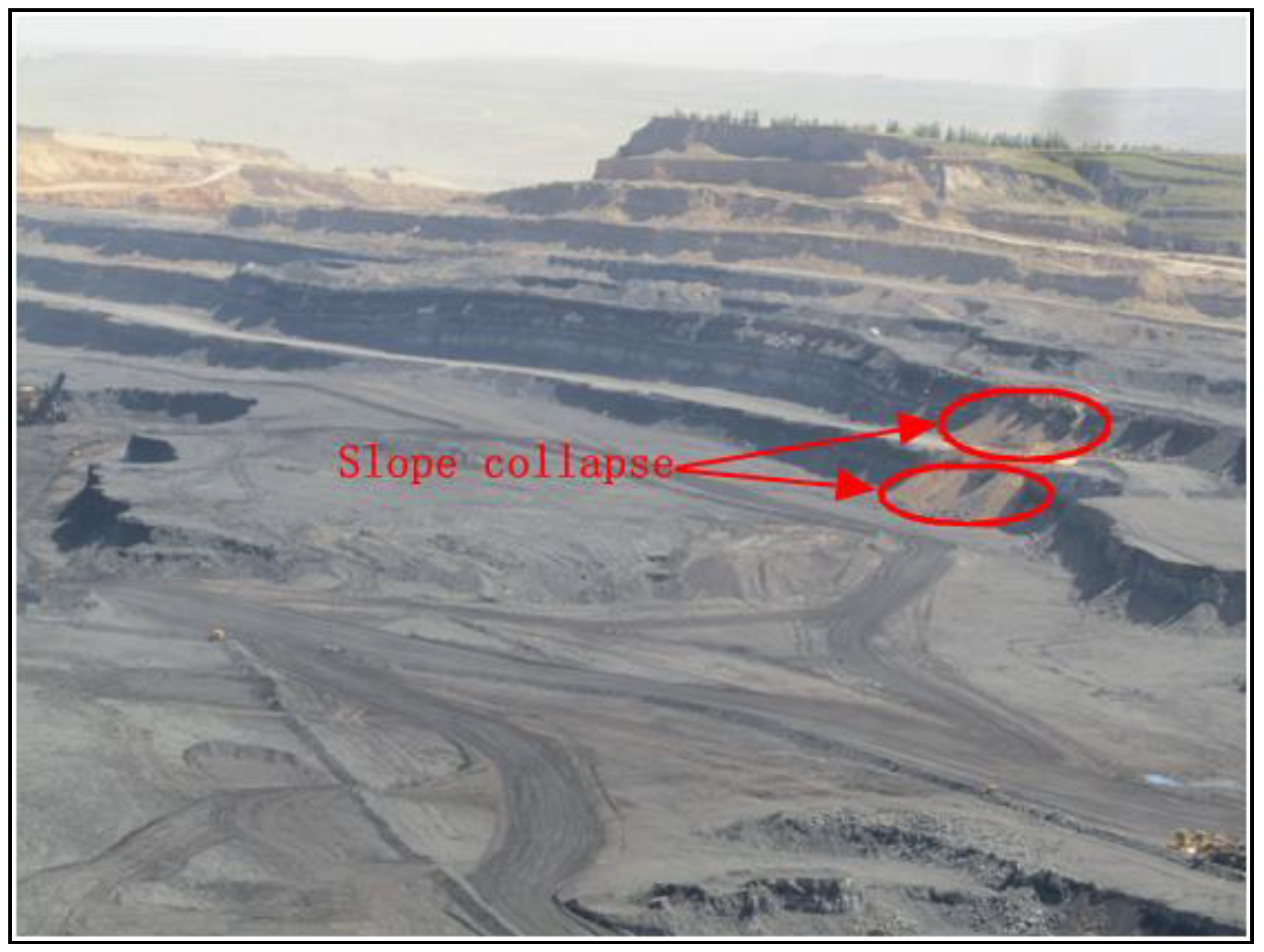
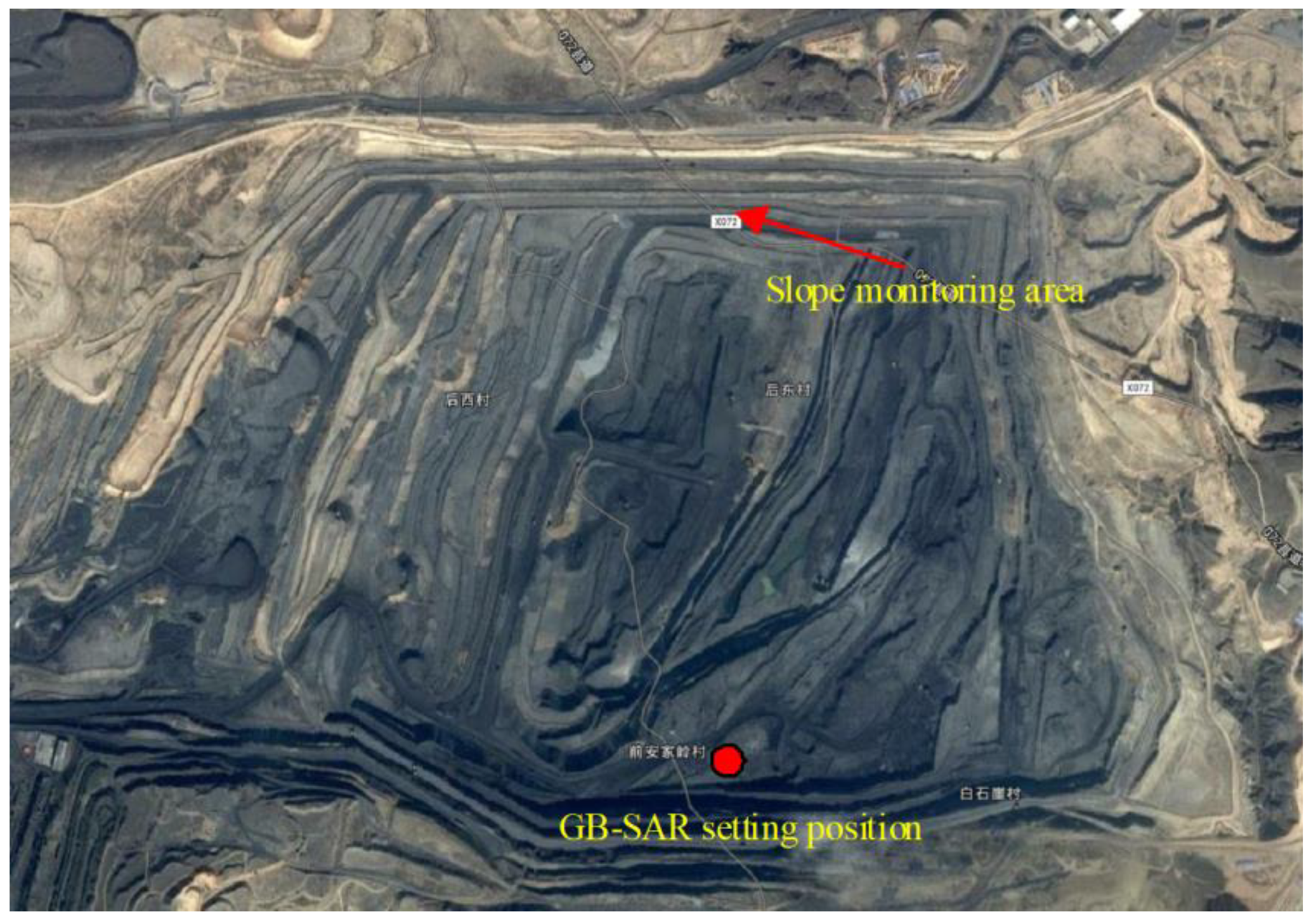
3.1. Geological Survey of Anjialing Mine

Anjialing open-pit coal mine is located at north latitude 39°26′03″ and east longitude 112°20′52″ in Shuozhou city, Shanxi Province, China. The total area of Anjialing is about 28 km² and its mining area is about 7842 m from east to west and 6556 m from north to south. Anjialing mine belongs to a temperate, semi-arid, continental, monsoon climate zone. It is drought-prone, cold, and windy in spring and winter and rainy, cool, and less windy in summer and fall [4]. The average annual rainfall in this area is about 435 mm. The highest annual rainfall in historical records was 757.4 mm, and the lowest annual rainfall was 195.6 mm. In the Anjialing mining area, 75% of the annual rainfall is in summer. The annual average temperature is about 6 °C. The temperature difference between day and night is about 20 °C, the maximum temperature is about 37.9 °C, and the minimum temperature is −32.4 °C.

Anjialing coal mine belongs to the hydrogeological unit of the Shentou spring area in the Sanggan river basin. The major aquifers in the area include Neogene aquifer, quaternary unconsolidated rock-type pore aquifer, carboniferous Permian clastic rock fissure aquifer, and Ordovician carbonate karst fissure aquifer systems. Its recharge sources are mainly atmospheric precipitation and surface river water infiltration. Due to low and concentrated atmospheric precipitation in this area, it is not conducive to the infiltration supply of atmospheric precipitation. The silty soil layer on the surface of the northern slope of Anjialing is characterized by large porosity, and a relative aquifer is formed after some rainfall infiltrates. The permeability coefficient is 1.2~2.0 × 10⁻⁵ m/s, and there is no water outlet point on the slope. There are several water outlet points in the bedrock joints and fissures in the northern end, among which the no. 4 coal seam is the most serious, indicating that there is static water in the bedrock. However, from the perspective of the static water level in the borehole, the water level is in the floor of the no. 4 coal seam, and the water level is relatively low, indicating that the water content in the rock mass is very low.

The study region belongs to the low mountains and hills of the Shanxi loess plateau. This region is mostly covered by loess, which is subject to strong erosion. In addition, there is sparse vegetation and many loess plateau geomorphologic landscapes. The gully region is in the mature stage in this region, and it takes on a V shape. The cutting depth of the gully is between 40 and 70 m. The topography of this region is basically high in the north and low in the south. The highest point in the study area is Shifeng in the north, with an elevation of 1537 m, while the lowest point is the Maguan river, which is in the southern part of the Xuegaodeng village, with an elevation of 1213 m. Hence, the maximum relative height difference is 324 m. According to the digital elevation model (DEM) analysis of the northern slope of Anjialing [27], the highest elevation of the slope is 1441 m, the lowest elevation is 1193 m, and the maximum relative height difference is 248 m. Figure 4 shows the topography of the northern slope of Anjialing.

Sliding landslides with a gentle slope are prone to occur in soft rock area, whereas collapse landslides are prone to occur in hard rocks. Anjialing is located in the loess plateau area, and hence, the study area is prone to sliding landslide disasters. The basic geological environment characteristics of the Anjialing mine area are expounded from the aspects of physical geography, formation lithology, geological structure, and geotechnical engineering. These characteristics can be used for monitoring and predicting the slope deformation. In this work, considering that the Luzigou anticline and Anjialing thrust only affect the southern slope, but the hydrogeological and meteorological factors are the main contributors to the deformation in the north slope, in the subsequent analysis, the geological structure factor is not included in the prediction model.

3.2. Data Acquisition

A GB-SAR monitoring data acquisition system was used to collect the deformation data of the Anjialing mine. The GB-SAR system consisted of two modules: a deformation data acquisition module and a meteorological data acquisition module.

The deformation data collecting module adopted the image by interferometric survey for mines (IBIS-M), which consists of a synthetic aperture radar (SAR) scanning unit and a linear rail (2 m in length). This module can collect four parameters, namely the slope shape coefficient, deformation rate, reverse deformation rate, and amplitude. The GB-SAR system can choose these parameters to monitor a single deformation point or their average values to monitor a certain region. Figure 5 depicts the linear scanning unit and scanning track of the IBIS-M for real-time deformation monitoring of the Anjialing mine slope.

The meteorological data acquisition module provides the data basis for the atmospheric phase correction in the GB-SAR system. A meteorological station (Vantage Pro2) was installed in the GB-SAR system to collect real-time meteorological data. Figure 6 shows a picture of the real products of the Vantage Pro2. It is an automatic weather station that integrates various weather sensors. This module can collect the following meteorological parameters: rainfall, temperature, atmospheric pressure, relative humidity, wind speed, and wind direction.

3.3. Field Geology Tests

The experiment test was carried out for the Anjialing open-pit mine, which belongs to China Coal Pingshuo Group Co., Ltd. in northern China. The main mining work face is in the north slope of Anjialing. According to the topography and mining situation, IBIS-M was installed in a relatively stable bedrock in the south to monitor the north slope. Figure 7 describes the location of the GB-SAR system in the mining area and the Anjialing north side slope. The distance between the GB-SAR system to the monitoring area was 2.3 km, which was within the monitoring range of the GB-SAR system.

A continuous experiment test was carried out during from 20 July to 26 July 2015. Rainfall was one of the most important inducing factors that affected the deformation of the open-pit slope. During the data collection period, rainfall occurred in the study area. Thus, the collected experimental data can reflect the influence effect of rainfall on the slope deformation. Figure 8 describes two locations where the collapse occurred on the north slope in Anjialing during the experimental period. Thus, the collected experimental datasets contained important information for the slope deformation prediction. The prediction result may show the potential of the proposed method for practical application.

In the experiments, the deformation data were collected by IBIS-M, and the meteorological factor data were collected by the Vantage Pro2 meteorological station. The meteorological factor data included the rainfall, temperature, atmospheric pressure, relative humidity, wind speed, and direction.

In addition, the hydrologic data were also collected by the hydrologic sensors installed in the underground structure of the Anjialing mine. The hydrologic data included the groundwater temperature and the groundwater level. This is because the groundwater may significantly affect the slope deformation. On the one hand, Anjialing is located in the loess plateau area, and the thickness of loess in this area usually ranges from 50 to 80 m. The structure of the loess layer is porous, and there are many cracks and biogenic holes. Therefore, when water flows in the loess layer, it not only runs along various pores, but also along cracks and holes. Groundwater is very important for the balance and stability of the underground structure. The increase and decrease of the groundwater level can destroy the equilibrium state that has been reached inside the slope. It can cause slope subsidence and deformation to reach a new dynamic equilibrium.

On the other hand, the groundwater temperature varies little from year to year, and it usually stays in the range of 8–12 °C. The temperature may affect the slope deformation from two aspects. The first is the contraction principle of groundwater. The temperature of groundwater will directly affect the temperature of the surrounding loess layer, resulting in thermal expansion and cold contraction of the loess layer, which may directly cause the deformation of the slope. Secondly, the groundwater temperature may affect the chemical reaction of the underground structure. The changes in groundwater temperature can promote or inhibit the chemical reactions between groundwater and pores and fractures, which may indirectly lead to the deformation of the slope.

4. Result and Discussion

In this work, the field datasets were used to train and test the proposed ensemble prediction model. The ensemble predicted results were also compared with those of each single-member prediction model.

Table 2. Inputs and output of the prediction models.

Prediction Model	Inputs	Outputs
BPNN	12 parameters from the geographical, climatic, and hydrographic aspects	Deformation
SVM
RNN
ANFIS
RVM
Ensemble

lists the inputs and outputs of each prediction model. The inputs were the 12 parameters collected by the GB-SAR and hydrologic sensors. These 12 inputs included the slope shape coefficient, deformation rate, reverse deformation rate, deformation amplitude, rainfall, temperature, atmospheric pressure, relative humidity, wind speed and direction, and groundwater temperature and level. The output was the deformation, which was calculated by the differential phase interferometric survey (DPIS) [26].

A total of 150 field datasets were collected by the GB-SAR system. Among those, 50 datasets were used for training, 50 for validation, and the other 50 for testing. The parameter settings for each member algorithm are given in

Table 3. Parameter settings for each member algorithm in the ensemble.

Learner	Parameter
BPNN	Number of hidden neurons is 20
SVM	Gaussian kennel with 0.5 kennel width
RNN	Number of hidden notes is 8
ANFIS	Number of Fuzzy rules is 10
RVM	Prior variance σ = 0.1

.

Table 4. Prediction results.

Learner	Optimal Weights	Validation Results (RMSE)	Testing Results (RMSE)
BPNN	0	4.42 mm	4.58 mm
SVM	0.01	3.93 mm	3.87 mm
RNN	0.35	2.79 mm	3.00 mm
ANFIS	0.12	3.26 mm	3.16 mm
RVM	0.52	2.65 mm	2.64 mm
Ensemble		2.01 mm	2.23 mm

provides the weight optimization result and the ensemble prediction result. The root-mean-square error (RMSE) was used as the optimization metric.

As can be seen in Table 4, the prediction errors of the five member algorithms for the test datasets varied from 2.64 to 4.58 mm. This is because different algorithms may be not effective for slope deformation prediction. For example, BPNN produces very low prediction accuracy, whereas RVM provides good accuracy. However, ensemble learning is able to distinguish the useful algorithms through weight optimization. As can be seen, BPNN was assigned a 0 weight, which means that this member algorithm was not included in the ensemble prediction model. In contrast, RVM received a largest weight of 0.52, because it produced the most accurate prediction result. RNN and ANFIS received the second and third largest weight values. The weight for SVM was 0.01, which was the second worst weight due to the model’s unsatisfactory prediction accuracy. As a result, only effective member algorithms were selected into the ensemble prediction model. The prediction accuracy was hence improved by the ensemble model, which produced the smallest prediction error 2.23 mm in comparison with the member models. It should also be noted that the prediction errors of the five member algorithms for the validation datasets were very close to those of the test datasets, which indicate that the obtained optimal weights were very effective for the GB-SAR datasets in this experiment. Thus, if new datasets are measured via the same GB-SAR system for the same open-pit mine, the established optimal ensemble model should be effective for slope deformation prediction using the data. However, if the open-pit mine changes, the member algorithms should be re-trained and the weight vector re-optimized.

It should emphasize that because diverse member algorithms are employed by the ensemble learning method, the robustness can be significantly enhanced by the ensemble prediction model. As can be seen in Table 4, although BPNN is not effective for slope deformation forecasting, the other three algorithms (RNN, ANFIS, and RVM) are adequate for this task. Hence, it is expected that the ensemble learning method will be effective for other prediction problems.

Furthermore, in order to investigate the mechanism of ensemble prediction in accuracy improvement, the prediction results of five test datasets are given in Figure 9 and

Table 5. Prediction results.

Learner	Predicted Deformation (mm)	Absolute Error (mm)	Average Absolute Error
BPNN	[0.69 16.35 10.06 9.87 15.94]	[4.73 10.62 2.53 0.23 2.50]	4.122 mm
SVM	[3.81 2.35 3.99 5.32 8.69]	[1.61 3.38 3.54 4.78 4.75]	3.612 mm
RNN	[5.33 6.51 8.25 10.76 14.08]	[0.09 0.78 0.72 0.66 0.64]	0.578 mm
ANFIS	[6.35 3.42 6.76 8.29 15.92]	[0.93 2.31 0.77 1.81 2.48]	1.660 mm
RVM	[5.22 5.65 7.10 9.82 12.22]	[0.20 0.08 0.43 0.28 1.22]	0.442 mm
Ensemble	[5.38 5.65 7.4300 9.92 13.28]	[0.04 0.08 0.10 0.18 0.16]	0.112 mm

. The actual deformation values of these five test datasets were 5.42, 5.73, 7.53, 10.10, and 13.44 mm, respectively.

As can be seen in Figure 9, BPNN produces very large prediction errors for the five datasets. The absolute errors were 4.73, 10.62, 2.53, 0.23, and 2.50 mm, as listed in Table 5. Moreover, the prediction values of datasets 2, 3, and 4 were later predictions, whereas for datasets 1 and 5, the results were early predictions. As a result, the prediction performance of BPNN is a little stochastic. This is why the weight optimization result in Table 4 assigned a zero value to BPNN.

Compared with the other network algorithm, RNN performs better than BPNN in term of prediction accuracy. The average error of RNN was 0.578 mm for these five datasets—an improvement of 3.544 mm compared with that of BPNN. In Table 5, it can be observed that all five predictions of RNN were later predictions.

Furthermore, the predictive performance of SVM and ANFIS were not as good as that of RNN. Their average errors were respectively 3.612 and 1.660 mm. As can be seen in Figure 9, the predictions of SVM were early predictions, while ANFIS generated dynamic predictions.

One can also observe in Figure 9 that the prediction values of RVM were very close to the actual measurements. Its average error was 0.442, better than the 0.578 value of RNN, which explains why the optimal weight assigned to RVM was larger than that of RNN.

Based on the prediction results of the five member algorithms, it can be observed that diverse algorithms produced different early and later predictions for the test datasets. Hence, it is possible to improve the prediction accuracy by appropriately combining early and later predictions. For example, for the fifth test dataset, if the weights 0, 0.01, 0.35, 0.12, and 0.52 of the five member algorithms, respectively, are multiplied, the early and later predictions will compensate each other to improve the weighted sum result of 5.65 mm.

$$\mathrm{Ensemble}=0\times 15.94+0.01\times 8.69+0.35\times 14.08+0.12\times 15.92+0.52\times 12.22=13.28$$

(14)

The actual measurement is 13.44 mm. Thus, the absolute error of the ensemble prediction is 0.16 mm, which shows a 75% improvement compared with the best prediction of 0.64 produced by RNN. Thanks to the optimal weight vector, the ensemble prediction drew the early and later predictions towards the actual deformation curve. As a result, the ensemble prediction results were closer to the actual one than those of the other algorithms. That is, the ensemble predictions were more accurate.

In Table 5, it can be observed that RVM produced an average absolute error of 0.422, which was the best of the five member algorithms. However, the ensemble model provided a better average error, 0.112, than that of RVM. The prediction accuracy was improved by at least 72.4% by the proposed ensemble learning method.

5. Conclusions

Mine slope deformation forecasting is of significant importance for mining safety. The GB-SAR system has been recognized as a powerful tool for mine slope monitoring, while the information fusion of GB-SAR monitoring parameters has been largely overlooked in the literature. To this end, this article proposed a new ensemble learning method to integrate five popular machine learning algorithms into a unified framework. Thanks to the diversity of the member algorithms and SQP-based weight optimization, the proposed ensemble model was able to demonstrate a more robust and accurate prediction performance than any of the member algorithms. Field data acquired from the collapse landslide in the Anjialing open-pit mine were used to evaluate the proposed method. The analysis results demonstrate that the predictive performance of the ensemble model was superior to all the member models. Because diverse machine learning algorithms can be incorporated into the ensemble framework, the proposed method can be extended to many prediction problems, such as coal price estimation. Future research will investigate the selection of member algorithms in the ensemble framework. The ensemble model will also be applied to predicting different landslides with similar/different dimensions and types.

References

1. Vaziri, A.; Moore, L.; Ali, H. Monitoring systems for warning impending failures in slopes and open pit mines. Nat. Hazards 2010, 55, 501–512. [Google Scholar]
2. Xu, Q. Theoretical studies on prediction of landslides using slope deformation process data. J. Eng Geol. 2012, 20, 145–151. [Google Scholar]
3. Yang, Y.; Wang, Z. Grey prediction research of slope deformation. Electron. J. Geotech. Eng. 2013, 18, 1255–1266. [Google Scholar]
4. Dick, G.; Erik, E.; Albert, G.; Doug, S.; Nick, D. Development of an early-warning time-of-failure analysis methodology for open-pit mine slopes utilizing ground-based slope stability radar monitoring data. Can. Geotech. J. 2014, 52, 515–529. [Google Scholar] [CrossRef]
5. Carlà, T.; Farina, P.; Intrieri, E.; Ketizmen, H.; Casagli, N. Integration of ground-based radar and satellite InSAR data for the analysis of an unexpected slope failure in an open-pit mine. Eng. Geol. 2018, 235, 39–52. [Google Scholar] [CrossRef]
6. Nie, L.; Li, Z.; Lv, Y.; Wang, H. A new prediction model for rock slope failure time: A case study in West Open-Pit mine, Fushun, China. Bull. Eng. Geol. Environ. 2017, 76, 975–988. [Google Scholar] [CrossRef]
7. Casagli, N.; Catani, F.; Del Ventisette, C.; Luzi, G. Monitoring, prediction, and early warning using ground-based radar interferometry. Landslides 2010, 7, 291–301. [Google Scholar] [CrossRef]
8. Zheng, D.; Gu, C.; Wu, Z. Time series evolution forecasting model of slope deformation based on multiple factors. Chin. J. Rock Mech. Eng. 2005, 24, 3180–3184. [Google Scholar]
9. Kong, F.; Lu, D.; Du, X.; Shen, C. Displacement analytical prediction of shallow tunnel based on unified displacement function under slope boundary. Int. J. Numer. Anal. Methods Geomech. 2019, 43, 183–211. [Google Scholar] [CrossRef]
10. Osasan, K.S.; Stacey, T.R. Automatic prediction of time to failure of open pit mine slopes based on radar monitoring and inverse velocity method. Int. J. Min. Sci. Technol. 2014, 24, 275–280. [Google Scholar] [CrossRef]
11. Strenk, P.; Wartman, J. Uncertainty in seismic slope deformation model predictions. Eng. Geol. 2011, 122, 61–72. [Google Scholar] [CrossRef]
12. Du, J.; Yin, K.; Lacasse, S. Displacement prediction in colluvial landslides, three Gorges reservoir, China. Landslides 2013, 10, 203–218. [Google Scholar] [CrossRef]
13. Guo, T.; He, W.; Jiang, Z.; Chu, X.; Reza, M.; Li, Z. An improved LSSVM model for intelligent prediction of the daily water level. Energies 2019, 12, 112. [Google Scholar] [CrossRef]
14. Chen, H.; Zeng, Z. Deformation prediction of landslide based on improved back-propagation neural network. Cogn. Comput. 2013, 5, 56–62. [Google Scholar] [CrossRef]
15. Chen, H.; Zeng, Z.; Tang, H. Landslide deformation prediction based on recurrent neural network. Neural Process. Lett. 2015, 41, 169–178. [Google Scholar] [CrossRef]
16. Du, S.; Zhang, J.; Li, J.; Su, Q.; Zhu, W.; Chen, Y. The deformation prediction of mine slope surface using PSO-SVM model. J. Electr. Eng. 2013, 11, 7182–7189. [Google Scholar] [CrossRef]
17. He, X.; Hua, X.; He, X. Weighted multi-point grey model and its application to high rock slope deformation forecast. Rock Soil Mech. 2007, 28, 1187–1191. [Google Scholar]
18. Liu, C.; Jiang, Z.; Han, X.; Zhou, W. Slope displacement prediction using sequential intelligent computing algorithms. Measurement 2019, 134, 634–648. [Google Scholar] [CrossRef]
19. Hu, B.; Su, G.; Jiang, J.; Sheng, J.; Li, J. Uncertain prediction for slope displacement time-series using Gaussian process machine learning. IEEE Access 2019, in press. [Google Scholar] [CrossRef]
20. Du, S.; Zhang, J.; Deng, Z.; Li, J. A novel deformation prediction model for mine slope surface using meteorological factors based on kernel extreme learning machine. Int. J. Eng. Res. Afr. 2014, 12, 15. [Google Scholar] [CrossRef]
21. Liu, K.; Wei, B.; Liu, B. Analysis model of slope deformation time series based on the genetic-adaptive neuron-fuzzy inference system. J. Beijing Jiaotong Univ. 2012, 36, 56–62. [Google Scholar]
22. Li, Z.; Goebel, K.; Wu, D. Degradation modeling and remaining useful life prediction of aircraft engines using ensemble learning. J. Eng. Gas Turbines Power-Trans. ASME 2019, 141, 041008. [Google Scholar] [CrossRef]
23. Li, Z.; Wu, D.; Hu, C.; Terpenny, J. An ensemble learning-based prognostic approach with degradation-dependent weights for remaining useful life prediction. Reliab. Eng. Syst. Saf. 2019, 184, 110–122. [Google Scholar] [CrossRef]
24. Tipping, M.E. Sparse bayesian learning and the relevance vector machine. J. Mach. Learn. Res. 2001, 1, 211–244. [Google Scholar]
25. Jang, J. ANFIS: Adaptive-network-based fuzzy inference system. IEEE Trans. Syst. Man Cybern. Syst. 1993, 23, 665–685. [Google Scholar] [CrossRef]
26. Čerňanský, M.; Makula, M.; Beňušková, Ľ. Organization of the state space of a simple recurrent network before and after training on recursive linguistic structures. Neural Netw. 2007, 20, 236–244. [Google Scholar] [CrossRef]
27. Shao, Z.; Wang, D.; Wang, Y.; Zhong, X.; Tang, X.; Hu, X. Controlling coal fires using the three-phase foam and water mist techniques in the Anjialing Open Pit Mine, China. Nat. Hazards 2015, 75, 1833–1852. [Google Scholar] [CrossRef]
Figure 1. The flowchart of the proposed method for ensemble prediction. Where J is the number of member algorithms and w is the weight vector.
Energies 12 01288 g001
Figure 2. A typical architecture of type-3 adaptive network-based fuzzy inference system (ANFIS), where II denotes the algebraic product operator and D denotes the normalization operator, MFFi is the membership function of ith input variable.
Energies 12 01288 g002
Figure 3. A typical architecture of recurrent neural networks (RNNs).
Energies 12 01288 g003
Figure 4. North slope topography of the Anjialing open-pit mine.
Energies 12 01288 g004
Figure 5. Synthetic aperture radar and linear rail unit module.
Energies 12 01288 g005
Figure 6. Meteorological sensor module: (1) rain collector, (2) solar panel, (3) radiation shield, (4) sensors mounting shelf, and (5) module base.
Energies 12 01288 g006
Figure 7. Ground-based interferometric radar (GB-SAR) setting position and the monitored slope.
Energies 12 01288 g007
Figure 8. Two collapses occurred on the north slope in the Anjialing open-pit mine.
Energies 12 01288 g008
Figure 9. Prediction results among the BPNN, SVM, RNN, ANFIS, RVM, and ensemble algorithms.
Energies 12 01288 g009