Article

A Dynamic Adam Based Deep Neural Network for Fault Diagnosis of Oil-Immersed Power Transformers

1
Guangxi Key Laboratory of Power System Optimization and Energy Technology, Guangxi University, Nanning 530004, China
2
College of Electrical Engineering, Guangxi University, Nanning 530004, China
*
Author to whom correspondence should be addressed.
Energies 2019, 12(6), 995; https://doi.org/10.3390/en12060995
Submission received: 30 January 2019 / Revised: 8 March 2019 / Accepted: 8 March 2019 / Published: 14 March 2019

Abstract

:
This paper presents a Dynamic Adam and dropout based deep neural network (DADDNN) for fault diagnosis of oil-immersed power transformers. To solve the problem of incomplete extraction of hidden information with data driven, the gradient first-order moment estimate and second-order moment estimate are used to calculate the different learning rates for all parameters with stable gradient scaling. Meanwhile, the learning rate is dynamically attenuated according to the optimal interval. To prevent over-fitted, we exploit dropout technique to randomly reset some neurons and strengthen the information exchange between indirectly-linked neurons. Our proposed approach was utilized on four datasets to learn the faults diagnosis of oil-immersed power transformers. Besides, four benchmark cases in other fields were also utilized to illustrate its scalability. The simulation results show that the average diagnosis accuracies on the four datasets of our proposed method were 37.9%, 25.5%, 14.6%, 18.9%, and 11.2%, higher than international electro technical commission (IEC), Duval Triangle, stacked autoencoders (SAE), deep belief networks (DBN), and grid search support vector machines (GSSVM), respectively.

1. Introduction

Power transformers are important equipment in power systems; their operational conditions directly affect the security and stability of the power grid. A fault on a power transformer will result in power outage at the associated region, which may cascade to the power grid leading to a widespread blackout, causing great social and economic losses [1,2]. Therefore, it is necessary to investigate fault diagnosis technologies for power transformers.
For the oil-immersed transformer, it is rare to conduct hood adjustment and overhaul involving disassembly, which means that it is very difficult for us to directly examine the internal insulation, especially the winding oil-immersed insulation. Thus, we can only assess the insulation state by some indirect ways. Generally, various preventive tests including insulation dielectric spectrum analysis [3,4,5,6], partial discharge method [7,8], and dissolved gas analysis (DGA) can accurately reflect the performance and state of all aspects and parts of the power transformer to a certain extent. In these testing items, the dissolved gas analysis is an important approach of transformer internal fault diagnosis. It is very effective to find latent faults in transformers as well as their development trends [9,10,11]. Many technicians have used the DGA technique to determine the quantitative relationship between the content of these characteristic gases and the internal faults of power transformers. Some improved DGA-based means have been investigated, including IEC ratio [12], Rogers ratio [13], Duval Triangle [14,15], and Dornenburg ratio [16], which are the more commonly used fault diagnosis methods. However, these traditional methods have limitations. They may not be able to provide an interpretation to every possible combination of various ratios and may have excessively absolute coding boundary. Due to the objective uncertainty of transformer fault itself and the boundaries of the subjective judgment, it is difficult to meet the requirements of engineering application with the above ratio methods.
Since the transformer faults are complex and concealed, simple and crude methods have difficulty performing effective diagnosis. It is essential to explore the principles, methods and means from various disciplines that are helpful in the fault diagnosis of transformers. With the rapid development of computer science and the rise of machine learning, multiple intelligent approaches such as artificial neural network [17,18,19], support vector machine (SVM) [20,21,22], fuzzy theory [23,24,25], extreme learning machine [26], and Bayesian network [27] have been applied in practice. A smart fault diagnostic approach based on integrating five interpretation methods using neural networks is proposed in [28]. Ma et al. [29] presented an intelligent framework for transformer condition monitoring and assessment. Within their framework, different intelligent algorithms can be effectively deployed. Peimankar et al. [30] first used multi-objective particle swarm optimization (PSO) algorithm to select the best subset of features corresponding to each fault class of power transformers. Then, they used ensemble learning systems to classify actual faults of transformers. Sherif et al. [31] utilized the thermodynamic theory to evaluate the severity based on the energy associated with each transformer fault type. These intelligent methods remedy the disadvantages of the mentioned traditional DGA methods. Although back propagation neural network (BPNN) [32] has highly nonlinear fitting and self-adaptive ability, its convergence is slow and it can easily be trapped in the local optimum. SVM is effective in fault diagnosis with good generalization ability on small datasets. However, it does not perform well on multi-classification problems and it is difficult to select the appropriate parameters. Bayesian network is simple. However, it is not easy to calculate the prior probability. These shallow learning methods are problematic when used to solve complex multi-category problems. Transformer fault patterns are diverse with different fault causes, levels, locations, etc. Thus, more advanced diagnosis techniques for power transformer faults are demanded.
To overcome the shortcomings of shallow learning algorithms, deep neural network (DNN) [33,34] is proposed to effectively realize, mimic or approximate any complex function, achieving autonomous parameters initialization and individual training for each layer. Examples include current transformer (CT) saturation classification using unsupervised learning [35], transformer fault diagnosis using deep belief network with non-code ratio [36], and vibration signals over cloud environment [37]. Although these DNN based methods are progressive and useful for complex multi-category judgment problems in CT saturation classification and fault diagnosis, they fail to build an efficient model with dynamical and adaptive learning rates for different parameters.
Stochastic gradient-based optimization is the core of a DNN model and learning rate is a key factor in optimization algorithms [38,39,40]. This paper proposes a dynamic adaptive moment estimation optimization algorithm based DNN to dynamically change the learning rates. Firstly, we use the gradient first and second orders of moment estimate to calculate the adaptive learning rate for each parameter [41,42]. Secondly, we calculate the optimal interval and adopt the reciprocal attenuation method to dynamically adjust the learning rate of each parameter along with the training process. In addition, to prevent over-fitting, multiple reset layers are added to the DNN, which will set some of neurons signals to zero, which strengthens the links between neurons.
The rest of the paper is organized as follows: Section 2 presents the theoretical basis and framework of the deep neural network based on Dynamic Adam and dropout (DADDNN). The process of constructing the DADDNN for transformer fault diagnosis and the related experimental results are given in Section 3. Validation of model generalization performance is demonstrated in Section 4, where discussions along with performance comparison with IEC, Duval Triangle, SAE, DBN, and GSSVM methods are given. Conclusions are drawn in Section 5.

2. Feasibility Analysis of the DADDNN

2.1. Dynamic Adam Optimization Algorithm

We present the Dynamic Adam optimization algorithm for gradient-based optimization of stochastic objective functions, which aims at machine learning problems with large datasets or high-dimensional parameter spaces [41]. Compared with the constant learning rate in Adam, the Dynamic Adam has a variable learning rate during iterations. As the number of iterations increases, the learning rate decreases reciprocally in the optimal interval according to Equation (6). Dynamic Adam combines the advantages of dynamic planning [43] and two popular optimization algorithms of adaptive gradient (AdaGrad) [44] and root mean square prop (RMSProp) [45], which has the following advantages:
  • It is appropriate for non-stationary objectives and problems.
  • Parameter updates are independent of the gradient. The upper limit of step size is determined by the hyper-parameters, ensuring that the updated step size is within the stable range.
  • It is gradient diagonal scaling invariant and handles noisy samples or sparse gradients better.
  • The parameters are generalized and only a small amount of adjustments are needed for different datasets.

Specific Implementation of Dynamic Adam

The algorithm and the properties of its update rule are described as follows [41]:
Get gradients with respect to stochastic objective at iteration t.
g t = θ f t θ t 1 )
Update biased first moment estimate.
m t = β 1 · m t 1 + 1 β 1 · g t
Update biased second moment estimate.
v t = β 2 · v t 1 + 1 β 2 · g t 2
Compute bias-corrected first moment estimate.
m ^ t = m t 1 β 1 t )
Compute bias-corrected second moment estimate.
v ^ t = v t 1 β 2 t )
Adjust the learning rate dynamically.
η t = η 0 1 + λ · ( t 1 )
Update parameters.
θ t = θ t 1 η t · m ^ t v ^ t + ϵ = θ t 1 η t · 1 β 2 t / ( 1 β 1 t ) · m t v t + ϵ ^
where:
  • t: Iteration t
  • f ( θ ) : Stochastic objective function with parameters θ
  • η 0 : Initial learning rate
  • λ : Attenuation coefficient of learning rate
  • ϵ : A constant for numerical stability
  • β 1 , β 2 0 , 1 ) : Exponential decay rates for the moment estimates
  • m t : First moment estimation at iteration t
  • v t : Second moment estimation at iteration t
  • m ^ t : Bias-corrected first moment estimate at iteration t
  • v ^ t : Bias-corrected second moment estimate at iteration t
  • g t 2 : The element-wise square g t g t
The initial value of first and second moment estimates ( m t , v t ) are set to zero. These moment estimates are updated using the Dynamic Adam, where hyper-parameters β 1 , β 2 0 , 1 ) control the exponential decay rates. It is biased towards zero during the initial iterations when the decay rates are small. To increase the absolute value of the moment estimates and eliminate the initial deviation, bias-corrected Equations (4) and (5) are utilized.

2.2. Dropout Technique

Dropout is a novel technique that provides an efficient way of approximately combining exponentially different neural network architectures. During training, it randomly sets neurons to zero, deleting the connections between their incoming and outgoing neurons. The neurons to be dropout are subject to Bernoulli distribution, i.e., each neuron is maintained with a fixed probability p independent of other neurons [46].
Dropout technique reduces the complex co-adaptability between neurons and increases the robustness in the absence of individual connection information. When a neuron cannot rely on other specific neurons, it has to learn to be robust via useful links. This ensures the established DNN is strong and not over-fitted. A neural network with and without dropout are shown in Figure 1.

3. Realization and Discussions of Transformer Fault Diagnosis Based on DADDNN Model

3.1. Transformer Fault Type and Data Acquisition

The DGA data used in this paper are as follows: Dataset 1 comes from China Southern Power Grid Company and consists of 135 samples, which are related to power transformers used at voltages between 35 kV and 500 kV. Dataset 2 contains 118 samples from IEC TC 10 database [12]. Dataset 3 contains 533 samples from published papers [47] on dissolved gases with corresponding fault types. Combining datasets collected from different sources to a whole dataset can enhance the generalization ability of the DADDNN. Therefore, we put Datasets 1–3 together into the Total dataset.
Considering the influence of a transformer’s capacity, model, environment and other factors, we classified the transformer fault types into seven categories [16,48]: Partial discharge (PD), low-energy discharge (LD), high-energy discharge (HD), Thermal fault of low temperature (t < 300 C), thermal fault of medium temperature ( t 300 C and t 700 C), thermal fault of medium-low temperature (MLT), and thermal fault of high temperature (HT) (t > 700 C). In addition, it was also crucial to record the samples under normal condition (NC). This helped us determine whether the transformer was in a fault state. Thus, the normal condition was also added to the recognition classes. The sample distributions of different datasets are shown in Table 1.
There were 786 records in total, each containing dissolved gases ( H 2 , C H 4 , C 2 H 6 , C 2 H 4 , and C 2 H 2 ), as well the incipient faults of the corresponding transformers.

3.2. Selection of the Feature Vector

DNN has powerful sensing ability. It can directly extract high-level features from the original data. This method straightly uses the dissolved gases ( H 2 , C H 4 , C 2 H 6 , C 2 H 4 , C 2 H 2 ) as feature vectors.
To eliminate the calculation error and maintain the original characteristics of the samples, the original data were normalized as follows:
x n o r = x x m e a n x s t d
where x denotes the primary gas concentration, x n o r indicates the normalized value, and x m e a n and x s t d represent the average value and standard deviation of this kind of gas, respectively. The normalized vector is used as the DADDNN input.

3.3. Transformer Fault Diagnosis Instantiation Model

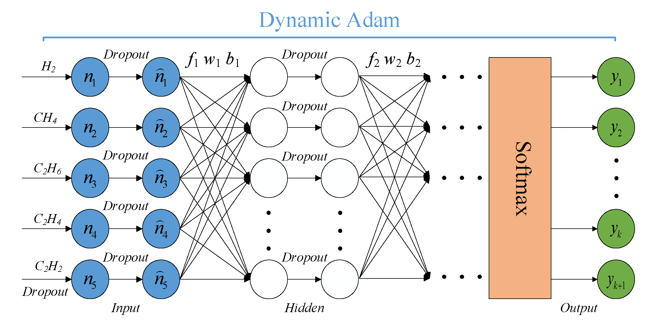
The DADDNN framework was constructed, as shown in Figure 2. The input vector n = n 1 , n 2 , n 3 , n 4 , n 5 represents the normalized value of the gas ( H 2 , C H 4 , C 2 H 6 , C 2 H 4 , C 2 H 2 ) concentrations. The output vector is y = y 1 , y 2 , , y k , y k + 1 , each of which is within (0, 1) range. The maximum value determines the attribution category. f i , w i , and b i indicate the activation function, weight, and bias of the ith layer (the input layer is marked as layer 0), respectively. As for the model parameters, the weights were initialized with the method of Glorot uniform distribution, the biases were initialized to 0, the batch training size was set to 30, and the probability of a neuron reset to zero was determined to be 50% [46,49]. To improve the performance, we adopted the parallel and deep network structure and used rectified linear units (Relu) as activation function. Meanwhile, Dynamic Adam was utilized for optimization algorithm.

3.3.1. Learning Rate

Learning rate is one of the most important hyper-parameters in deep learning. It is positive expectation that learning rates can change from big to small in the optimal interval. This can increase the convergence performance. Therefore, we further determined the initial learning rate η 0 and attenuation coefficient λ of Dynamic Adam by finding the optimal range.
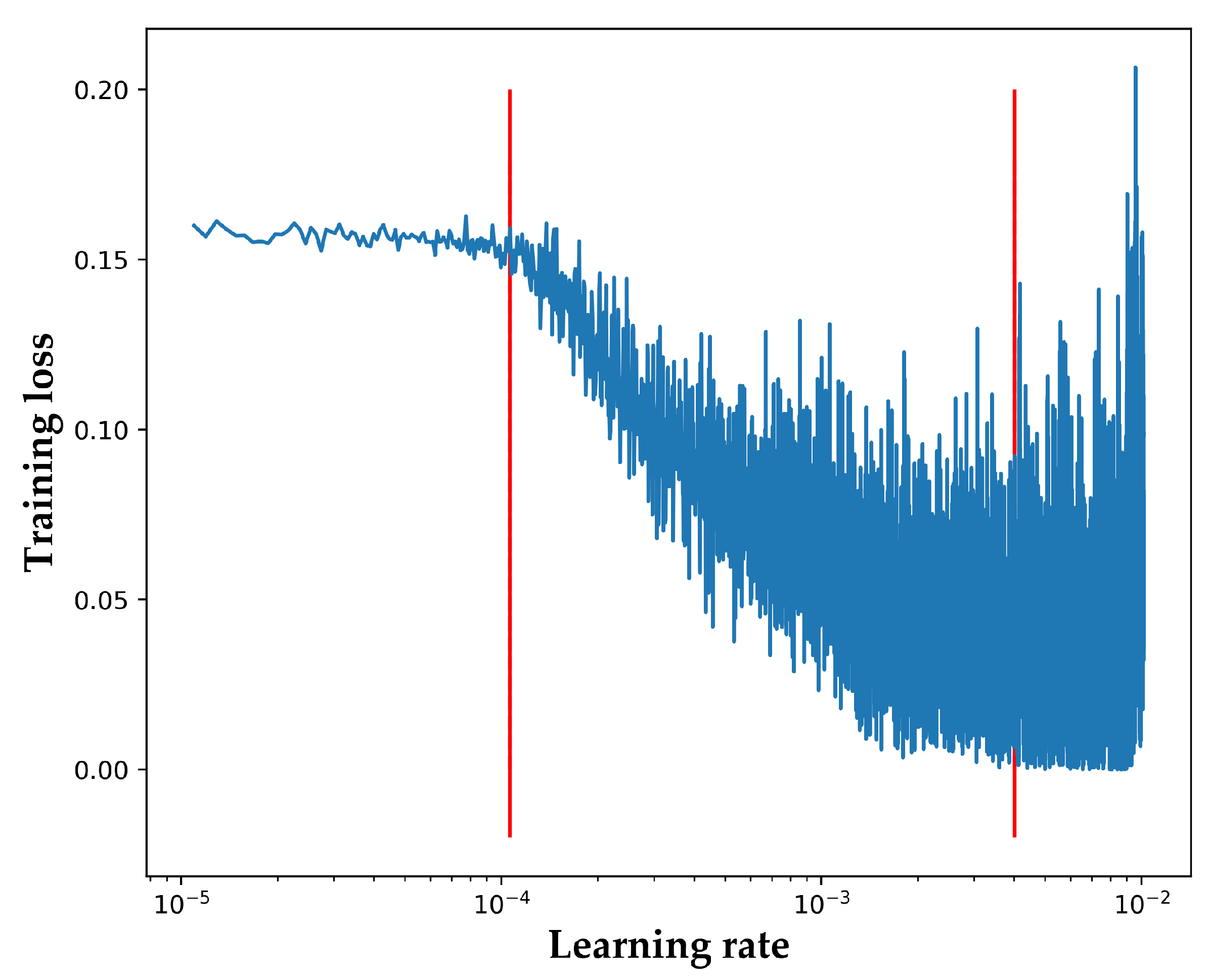
When the learning rate enters the optimal range, the training loss (network loss in training) will drop steeply and maintain a downward trend. We gradually increased the learning rate at every iteration and observed the rise and fall of the training loss to determine the optimal interval.
1 e p o c h = t r a i n i n g s a m p l e s b a t c h s i z e i t e r a t i o n s .
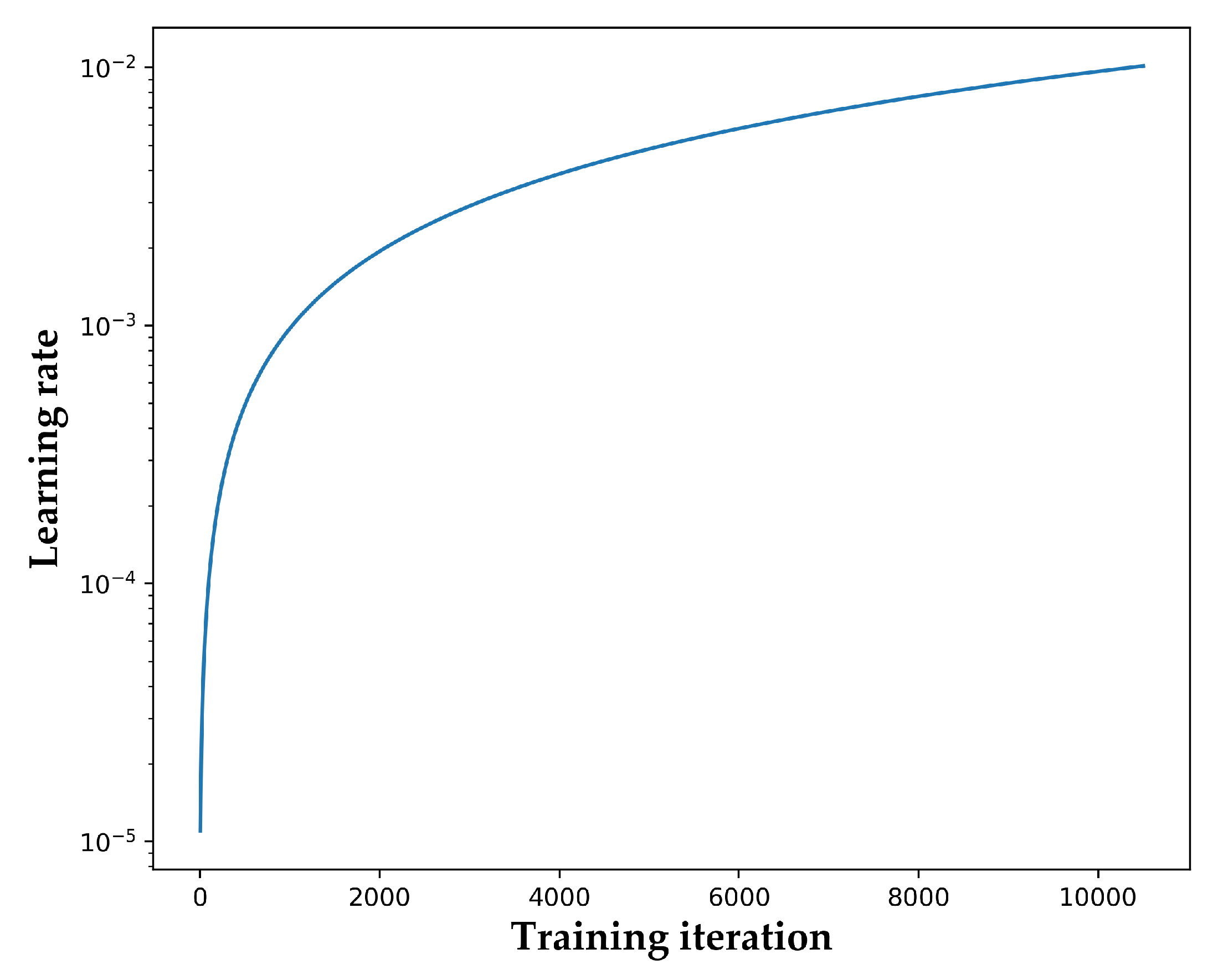
The dynamic learning rate presents the non-linear growth according to Equation (10) and is shown in Figure 3.
η = η m i n + η m a x η m i n · i t e r a t i o n s t o t a l i t e r a t i o n s
where η denotes the dynamic learning rate, and η m a x and η m i n indicate the maximum and minimum learning rates, which are set to 1 × 10 2 and 1 × 10 5 , respectively.
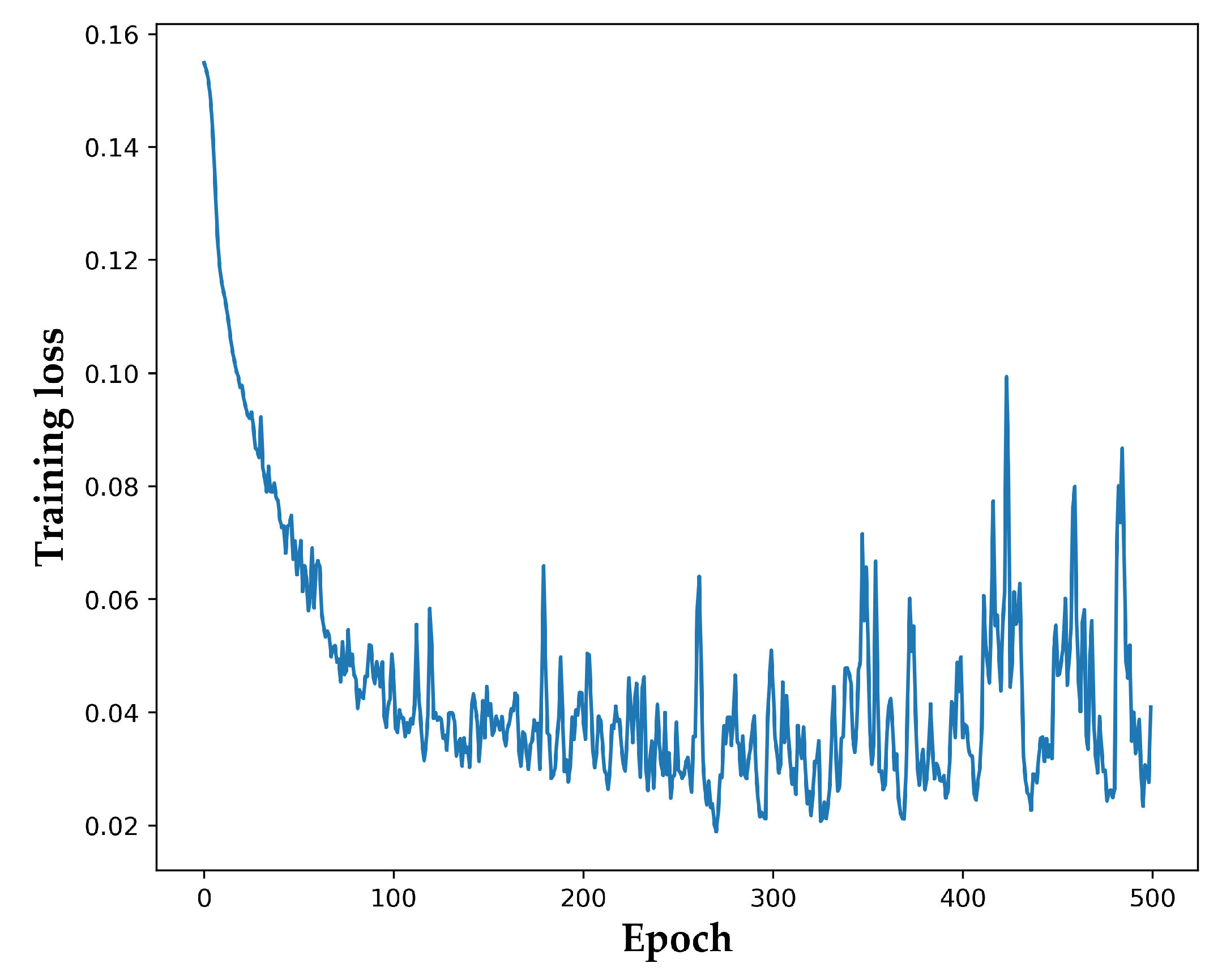
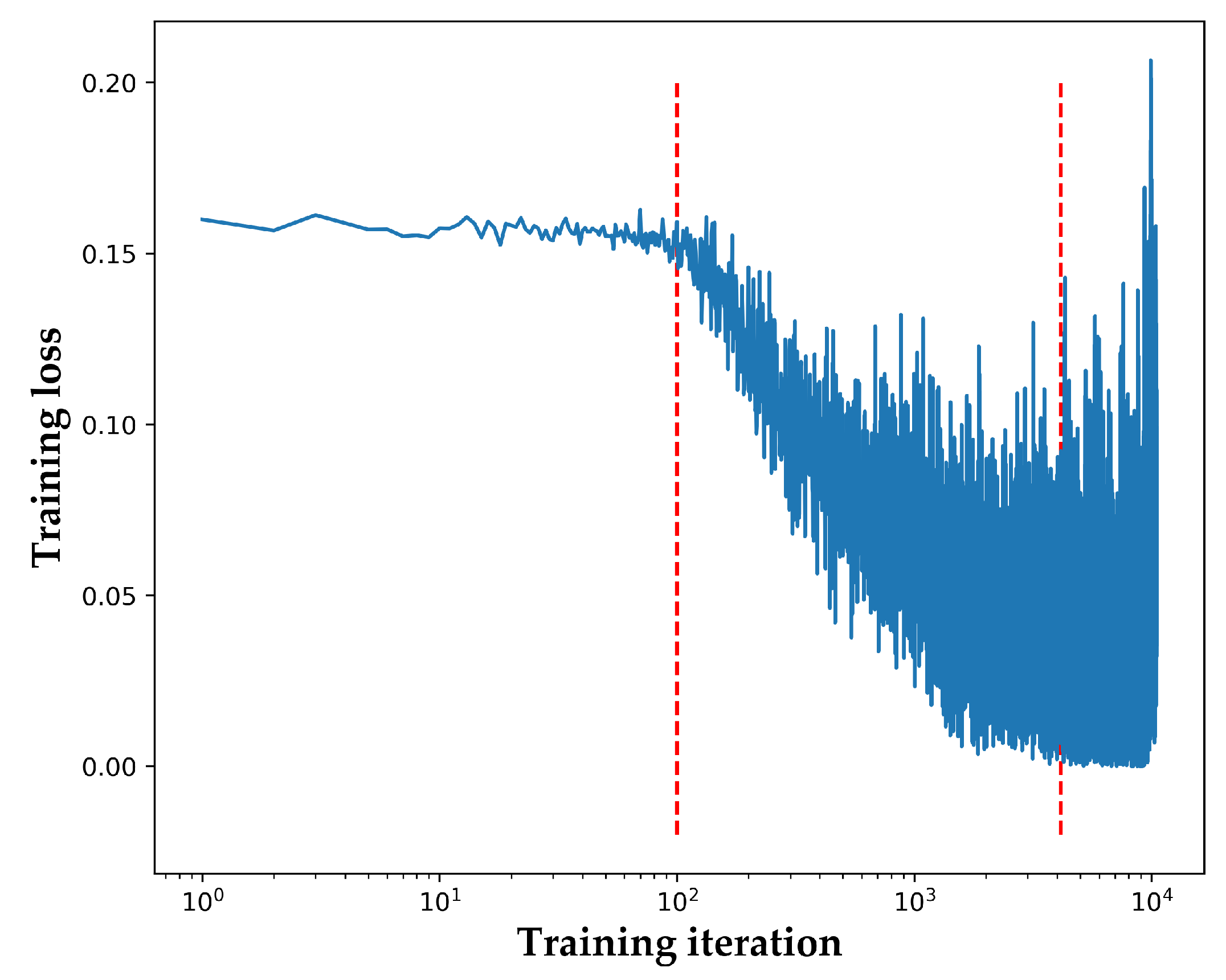
In the process of finding the optimal learning rate interval, Figure 4 shows the relationship between training epoch and training loss. The relationship between training iteration and training loss is shown in Figure 5.
By observing Figure 4, we preliminarily determined that the training loss fell rapidly during the training epochs [0, 200]. It can be clearly seen in Figure 5 that the training loss started to descend sharply from the 100th iteration. Through conversion, taking the 100th iteration and the 4140th iteration as nodes, we could precisely calculate the optimal interval of the learning rate, as shown in Figure 6.

3.3.2. Paratactic Network Structure

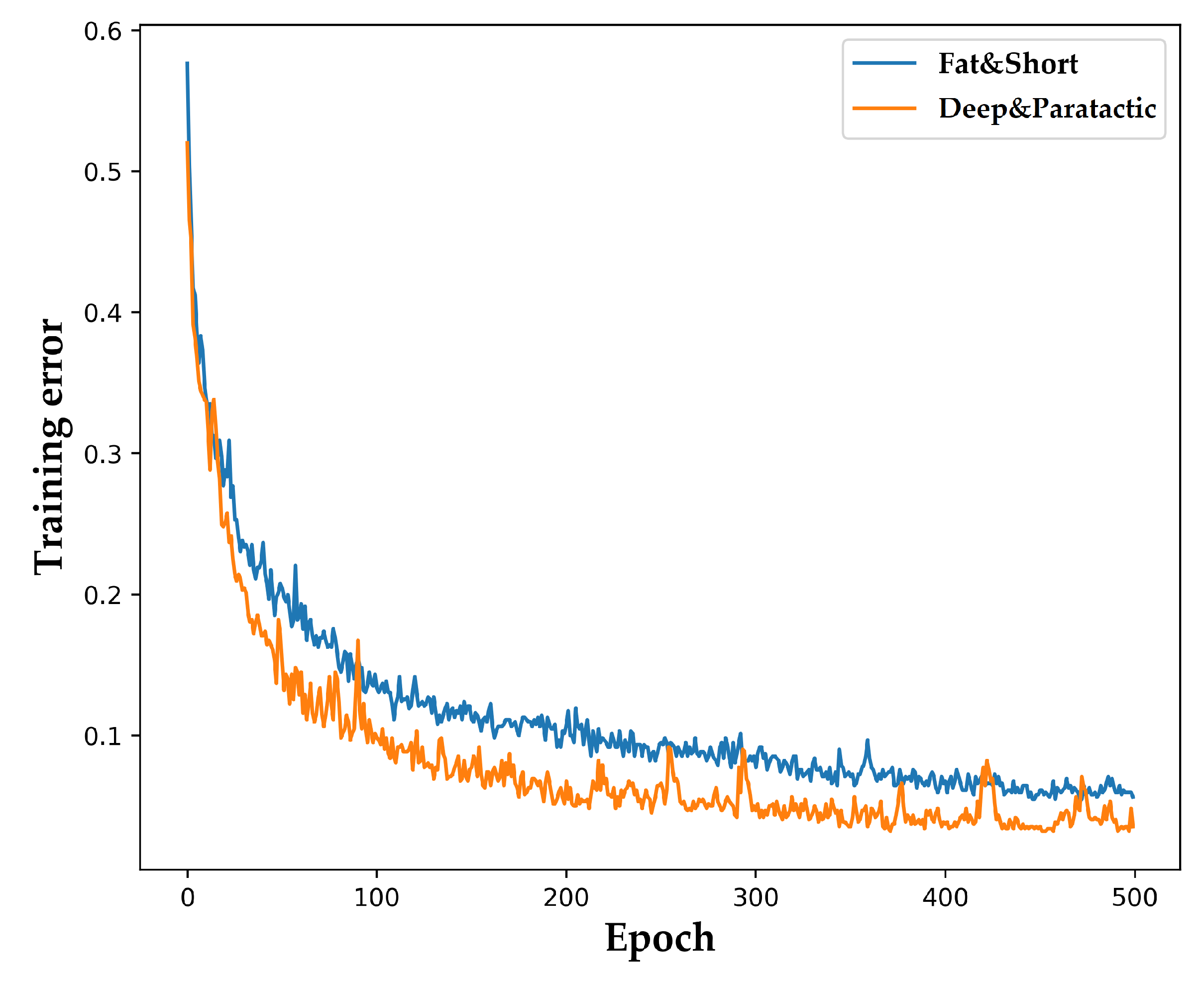
To construct the transformer fault diagnosis model, a paratactic network structure with 5 input layers, 5 hidden layers, and 500 neurons was utilized. Fat and short structure was used for comparison. Then, the number combination of neurons per hidden layer with paratactic structure was (100,100,100,100,100). Similarly, the other structure was (50,400,50). The convergence results are shown in Figure 7.
As shown in Figure 7, the convergence speeds were quite similar at the beginning. However, the performance difference was exhibited just after 16 learning epochs and the training error of the fat and short structure was higher than 5% at the end. The models with deep and paratactic structure had better performance as the training error was further reduced to 3%.

3.3.3. Activation Function “Relu”

In a DNN model, the commonly used activation functions are as follows:
S i g m o i d : f ( x ) = 1 1 + exp ( x )
S o f t p l u s : f ( x ) = log ( exp ( x ) + 1 )
R e l u : f ( x ) = m a x ( 0 , x )
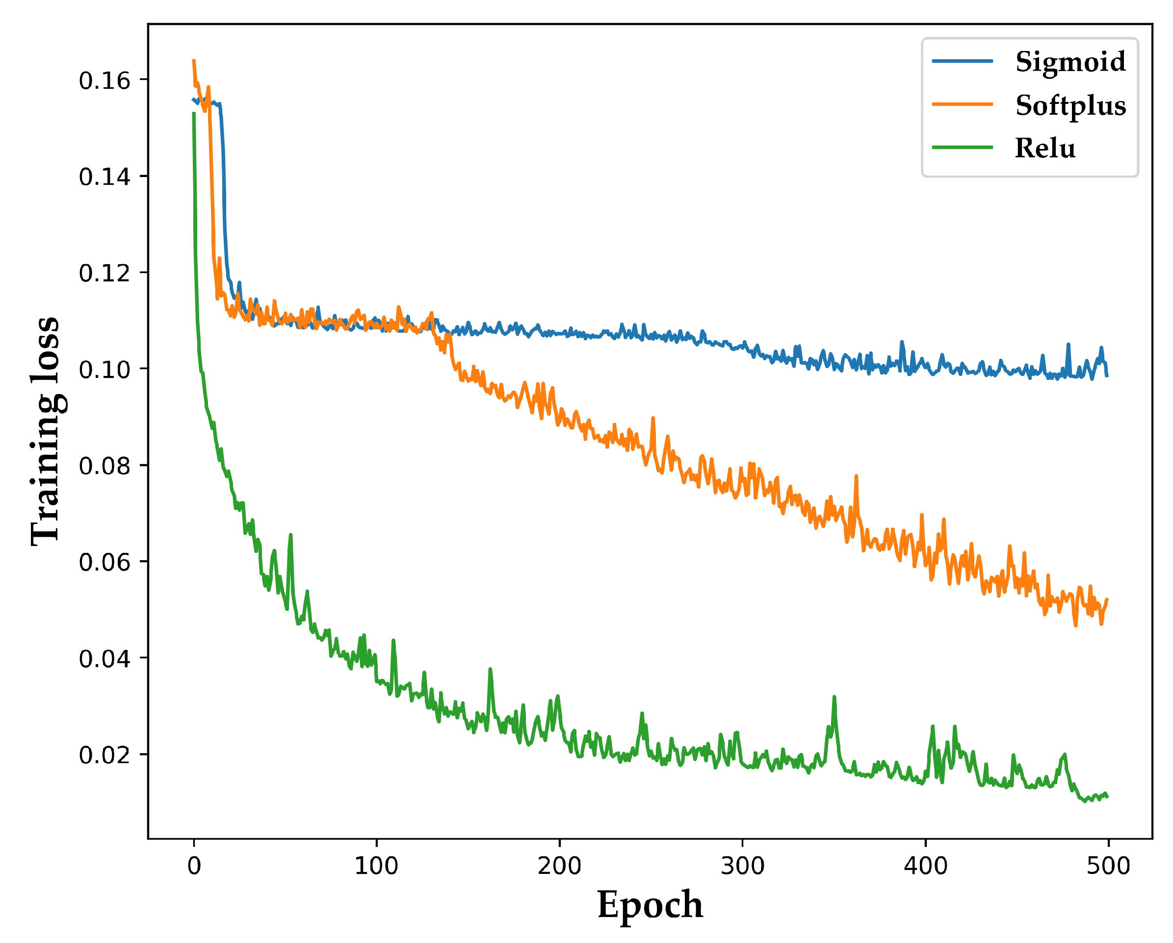
We adopted the Relu function to activate the DADDNN with the characteristic. The output was set to zero when the input value was less than zero; otherwise, the output was equal to the input. Meanwhile, Sigmoid and Softplus functions were also used for training. The convergence results are shown in Figure 8.
It is obviously seen in Figure 8 that Relu achieved a remarkable increment of convergence performance over Softplus in convergence speed and precision. Compared to Sigmoid, Relu relieved the phenomenon of sharp gradient and gradient disappearance.

3.3.4. Optimization Algorithm “Dynamic Adam”

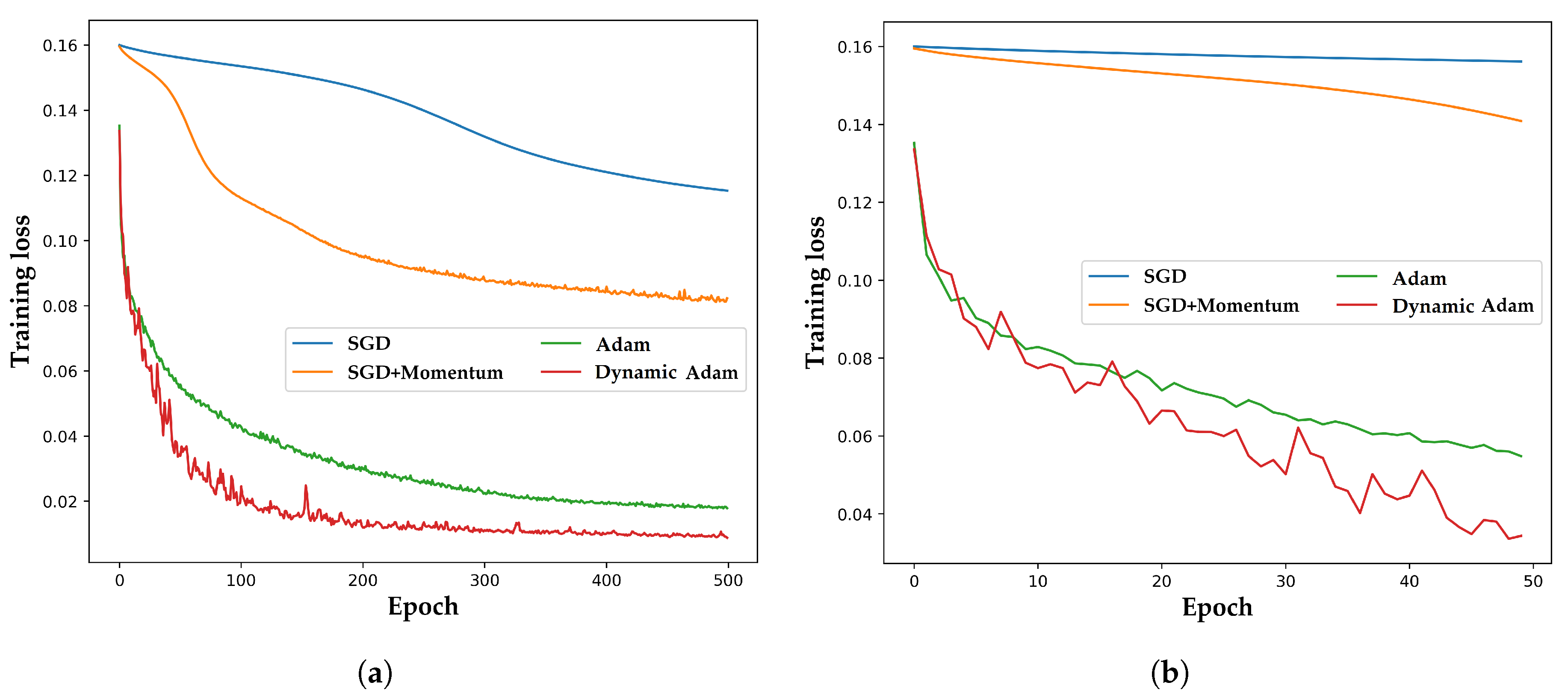
As for optimization algorithm, we utilized the proposed Dynamic Adam whose exponential decay rates β 1 and β 2 for the moment estimates were set to 0.9 and 0.999. The η 0 was initialized to 4.006× 10 3 . To improve the stability, λ and the constant for numerical stability ϵ were set to 10 3 and 10 8 , respectively [41]. At the same time, SGD, SGD+Momentum and Adam optimization algorithms were also applied to Dataset 2 for comparison.
As shown in Figure 9, the training loss based on Dynamic Adam lowered rapidly in the initial stage and kept convergence smooth after 300 epochs. In addition, Dynamic Adam outperformed SGD with Momentum by a large margin in the whole stage. One important reason was that it adopted different learning rates for different parameters instead of fix picking manually as in SGD. Compared to the Adam, Dynamic Adam had better convergence properties since learning rates could change dynamically.
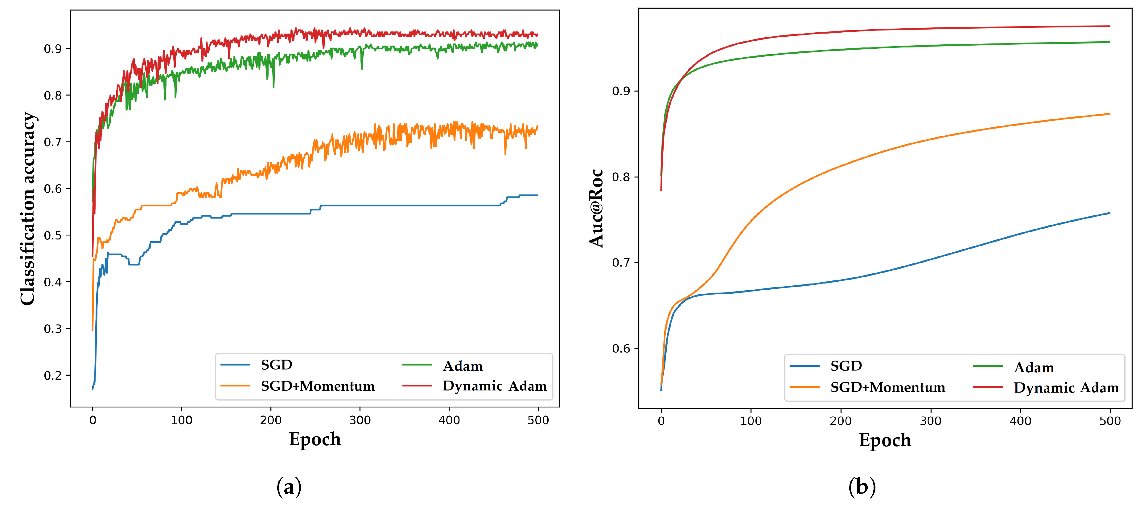
The classification accuracies for the four optimization algorithms are shown in Figure 10a. During the last 100 epochs, the upward trend converged to the stable point obviously. Precisely, the average accuracies were: 55.0% for SGD, 70.8% for SGD+Momentum, 86.8% for Adam, and 93.1% for Dynamic Adam. The area under the receiver operating characteristic curve (Auc@Roc) of Dynamic Adam achieved 97.5%, indicating its progressiveness.

4. DADDNN Model Effect Analysis

4.1. Method Performance Comparison

To further verify the effectiveness of the proposed approach, the IEC 60599 [16], Duval Triangle, SAE, DBN, GSSVM, and DADDNN methods were performed with our four datasets. The ratio between training set and testing set was kept at 3:1. We introduced random noise to train a 100 hidden unit SAE and used it to initialize a feed forward neuron network (FFNN). A DBN consisted of two 100-100 units restricted Boltzmann machines (RBMs) was trained to exploit the weight to initialize a FFNN. Meanwhile, we chose the radial basis function and adopted cross-validation to construct a GSSVM model. The penalty factor and the radius of kernel function were set by Grid Search. The results are shown in Table 2.
In Table 2, we can see that the diagnosis accuracies of DADDNN were the highest on all four datasets. Compared to the GSSVM model, the diagnosis accuracies of DADDNN increased by 11.0%, 10.8%, 12.8% and 10.2%, respectively. Compared to an unsupervised SAE model, the improvements were 11.0%, 21.5%, 12.0%, and 14.2%, respectively. We also compared our method with traditional approaches such as IEC 60599 and Duval Triangle, and the improvements of average accuracies were 37.9% and 25.5%, respectively. In other words, the more diversified network and more flexible optimization made the DADDNN obtain higher diagnosis accuracy.
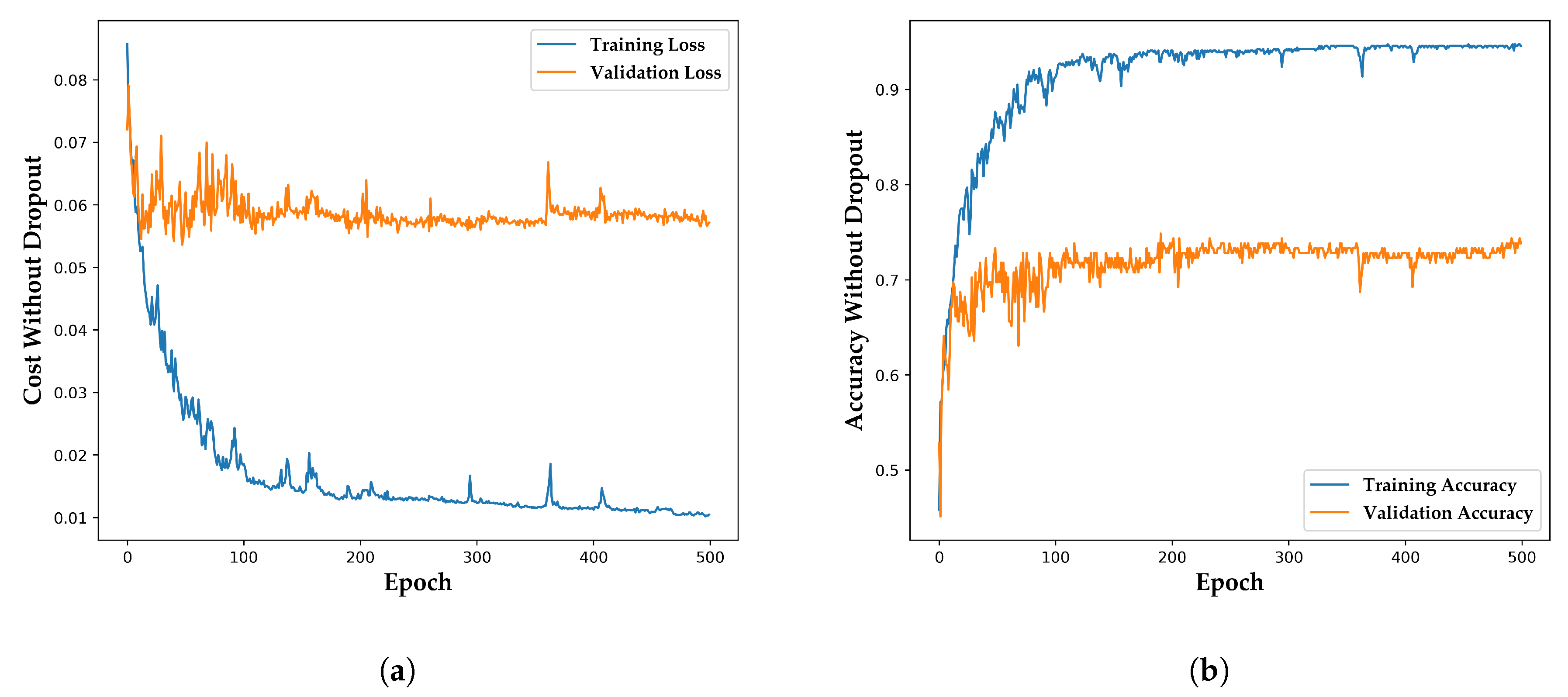
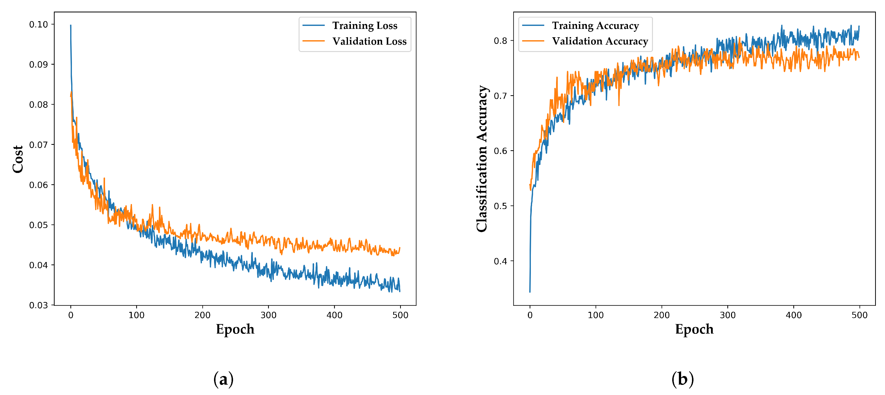
To fully demonstrate the effectiveness of the proposed DADDNN, extensive tests were performed. Table 3 lists the diagnosis accuracies for fault types of PD, LD, HD, LT, MT, MLT, HT, and NC in the Total dataset, as well diagnosis methods of IEC 60599, Duval Triangle, SAE, DBN and GSSVM for comparison. Meanwhile, the convergence process of DADDNN without and with dropout are shown in Figure 11 and Figure 12, respectively.
As shown in Table 3, the NC type accuracies of IEC 60599 and Duval Triangle were 0.0% because the normal condition judgement rules were missing for them. Therefore, these two traditional methods could not distinguish the normal state and are not suitable for real-time fault warning. Our model performed well, especially in the newly added MLT type compared with the other approaches. The difference between the maximum and minimum values of these compared methods in the single category diagnosis accuracy were 100%, 96.4%, 76.7%, 78.2%, and 72.1%, respectively. However, DADDNN could reduce to 40.9%, which illustrates that it has stable and balanced recognition ability for different fault categories.
As shown in Figure 11, the difference between training curve and validation cure of DADDNN without dropout was large. Average values gap of training accuracy and validation accuracy was 20.0%, indicating that the model is over-fitted. Conversely, the convergence process of DADDNN with dropout was normal (Figure 12), demonstrating that the dropout technique is suitable for preventing over-fitted.

4.2. Analysis of Generalization Performance

To test the general applicability of the Dynamic Adam for other classification problems, four benchmark cases were used, which are from university of California Irvine (UCI) database for machine learning [50]. These datasets include the medical Breast cancer data, biologic Iris data, Wine data, and chemical Glass identification data. The specific information of each dataset is shown in Table 4. Meanwhile, since the optimization algorithms SGD, SGD+Momentum, and Adagrad have a wide range of applications, the performance of the four DNN based algorithms were compared.
For the DNN model, we used the mean squared error (MSE) as the loss function, the benchmark learning rate was set to 0.01 and the value of Momentum was set to 0.8. All input data were normalized in [0, 1] before training. Table 5 shows the comparison results.
For the datasets of Iris and Wine with lesser categories and smaller samples, both the Adagrad and Dynamic Adam could fully extract data information and make accurate judgments, obtaining 100.0% classification accuracy in testing. Compared with the SGD and SGD+Momentum, performance was significantly improved. For the dataset of Breast cancer with lesser categories and larger samples, the Dynamic Adam achieved the highest 97.0% classification accuracy.For the dataset of Glass identification with more categories and smaller samples, it was more difficult to classify. Compared with 73.810% and 73.913% classification accuracies of other approaches [51,52], our approach had a better performance, reaching 81.4%.

5. Conclusions

This study considered how to recognize a transformer fault with data driven. Dynamic Adam and dropout based DNN is well-suited to the diagnosis problems. Some conclusions are as follows:
(1) By using Dynamic Adam, which aims at multi-dimensional parameter spaces, we solved the problem of dynamically planning the learning rates for different parameters. This speeds up the convergence.
(2) Compared with IEC, Duval Triangle, SAE, DBN and GSSVM models, the proposed approach had significant and balanced growth in diagnosis accuracy. It could reflect the real state of transformers more accurately.
(3) We exploited the DADDNN model to conduct pattern recognition for other datasets of different fields. Our method provides a practicable idea for intelligent diagnosis.
With the development of high-voltage power transmission, power transformer capacity is increasing and the associated operation, control and protection are more intelligent. Faults on a power transformer will have higher complexity and concurrency. Combining model driven with data driven methods is expected to play an important role in future research.

Author Contributions

Conceptualization, H.W.; Data curation, M.O.; Formal analysis, Y.Z.; Investigation, M.O.; Methodology, M.O.; Software, M.O.; Supervision, H.W.; Validation, H.W.; Writing—original draft, M.O.; and Writing—review & editing, J.T. and Y.Z.

Funding

This research received no external funding.

Conflicts of Interest

The authors declare no conflict of interest.

References

  1. Tang, S.; Hale, C.; Thaker, H. Reliability modeling of power transformers with maintenance outage. Syst. Sci. Control Eng. 2014, 2, 316–324. [Google Scholar] [CrossRef]
  2. Sang, Z.; Mao, C.; Lu, J.; Wang, D. Analysis and Simulation of Fault Characteristics of Power Switch Failures in Distribution Electronic Power Transformers. Energies 2013, 6, 4246–4268. [Google Scholar] [CrossRef] [Green Version]
  3. Liu, J.; Zheng, H.; Zhang, Y.; Wei, H.; Liao, R. Grey Relational Analysis for Insulation Condition Assessment of Power Transformers Based Upon Conventional Dielectric Response Measurement. Energies 2017, 10, 1526. [Google Scholar] [CrossRef]
  4. Linhjell, D.; Lundgaard, L.; Gafvert, U. Dielectric response of mineral oil impregnated cellulose and the impact of aging. IEEE Trans. Dielectr. Electr. Insul. 2007, 14, 156–169. [Google Scholar] [CrossRef]
  5. Liu, J.; Fan, X.; Zheng, H.; Zhang, Y.; Zhang, C.; Lai, B.; Wang, J.; Ren, G.; Zhang, E. Aging condition assessment of transformer oil-immersed cellulosic insulation based upon the average activation energy method. Cellulose 2019. [Google Scholar] [CrossRef]
  6. Zhang, Y.; Liu, J.; Zheng, H.; Wei, H.; Liao, R. Study on Quantitative Correlations between the Ageing Condition of Transformer Cellulose Insulation and the Large Time Constant Obtained from the Extended Debye Model. Energies 2017, 10, 1842. [Google Scholar] [CrossRef]
  7. Mehdizadeh, S.; Yazdchi, M.; Niroomand, M. A Novel AE Based Algorithm for PD Localization in Power Transformers. J. Electr. Eng. Technol. 2013, 8, 1487–1496. [Google Scholar] [CrossRef] [Green Version]
  8. Wang, K.; Li, J.; Zhang, S.; Liao, R.; Wu, F.; Yang, L.; Li, J.; Grzybowski, S.; Yan, J. A hybrid algorithm based on s transform and affinity propagation clustering for separation of two simultaneously artificial partial discharge sources. IEEE Trans. Dielectr. Electr. Insul. 2015, 22, 1042–1060. [Google Scholar] [CrossRef]
  9. Engineers, E.E.; Board, I.S. IEEE Guide for the Interpretation of Gases Generated in Oil-Immersed Transformers; IEEE: Piscataway, NJ, USA, 2009. [Google Scholar] [CrossRef]
  10. Liu, J.; Zheng, H.; Zhang, Y.; Li, X.; Fang, J.; Liu, Y.; Liao, C.; Li, Y.; Zhao, J. Dissolved Gases Forecasting Based on Wavelet Least Squares Support Vector Regression and Imperialist Competition Algorithm for Assessing Incipient Faults of Transformer Polymer Insulation. Polymers 2019, 11, 85. [Google Scholar] [CrossRef]
  11. Cheng, L.; Yu, T. Dissolved Gas Analysis Principle-Based Intelligent Approaches to Fault Diagnosis and Decision Making for Large Oil-Immersed Power Transformers: A Survey. Energies 2018, 11, 913. [Google Scholar] [CrossRef]
  12. Duval, M.; Depabla, A. Interpretation of gas-in-oil analysis using new IEC publication 60599 and IEC TC 10 databases. Electr. Insul. Mag. IEEE 2002, 17, 31–41. [Google Scholar] [CrossRef]
  13. Rogers, R.R. IEEE and IEC Codes to Interpret Incipient Faults in Transformers, Using Gas in Oil Analysis. IEEE Trans. Electr. Insul. 2007, EI-13, 349–354. [Google Scholar] [CrossRef]
  14. Duval, M. A review of faults detectable by gas-in-oil analysis in transformers. Electr. Insul. Mag. IEEE 2002, 18, 8–17. [Google Scholar] [CrossRef]
  15. Duval, M.; Lamarre, L. The duval pentagon-a new complementary tool for the interpretation of dissolved gas analysis in transformers. IEEE Electr. Insul. Mag. 2014, 30, 9–12. [Google Scholar] [CrossRef]
  16. Faiz, J.; Soleimani, M. Dissolved Gas Analysis Evaluation using Conventional Methods for Fault Diagnosis in Electric Power Transformers- A Review. IEEE Trans. Dielectr. Electr. Insul. 2017, 24, 1239–1248. [Google Scholar] [CrossRef]
  17. Barbosa, F.R.; Almeida, O.M.; Braga, A.P.D.S.; Amora, M.A.B.; Cartaxo, S.J.M. Application of an artificial neural network in the use of physicochemical properties as a low cost proxy of power transformers DGA data. IEEE Trans. Dielectr. Electr. Insul. 2012, 19, 239–246. [Google Scholar] [CrossRef]
  18. Miranda, V.; Castro, A.R.G.; Lima, S. Diagnosing Faults in Power Transformers With Autoassociative Neural Networks and Mean Shift. IEEE Trans. Power Deliv. 2012, 27, 1350–1357. [Google Scholar] [CrossRef]
  19. Lin, J.; Sheng, G.; Yan, Y.; Dai, J.; Jiang, X. Prediction of Dissolved Gas Concentrations in Transformer Oil Based on the KPCA-FFOA-GRNN Model. Energies 2018, 11, 225. [Google Scholar] [CrossRef]
  20. Ganyun, L.V.; Haozhong, C.; Haibao, Z.; Lixin, D. Fault diagnosis of power transformer based on multi-layer SVM classifier. Electr. Power Syst. Res. 2005, 74, 1–7. [Google Scholar] [CrossRef]
  21. Fei, S.; Zhang, X. Fault diagnosis of power transformer based on support vector machine with genetic algorithm. Expert Syst. Appl. 2009, 36, 11352–11357. [Google Scholar] [CrossRef]
  22. Fang, J.; Zheng, H.; Liu, J.; Zhao, J.; Zhang, Y.; Wang, K. A Transformer Fault Diagnosis Model Using an Optimal Hybrid Dissolved Gas Analysis Features Subset with Improved Social Group Optimization-Support Vector Machine Classifier. Energies 2018, 11, 1922. [Google Scholar] [CrossRef]
  23. Rigatos, G.; Siano, P. Power transformers’ condition monitoring using neural modeling and the local statistical approach to fault diagnosis. Int. J. Electr. Power Energy Syst. 2016, 80, 150–159. [Google Scholar] [CrossRef]
  24. Li, E.; Wang, L.; Song, B.; Jian, S. Improved Fuzzy C-Means Clustering for Transformer Fault Diagnosis Using Dissolved Gas Analysis Data. Energies 2018, 11, 2344. [Google Scholar] [CrossRef]
  25. Khan, S.A.; Equbal, M.D.; Islam, T. A comprehensive comparative study of DGA based transformer fault diagnosis using fuzzy logic and ANFIS models. IEEE Trans. Dielectr. Electr. Insul. 2015, 22, 590–596. [Google Scholar] [CrossRef]
  26. Li, S.; Wu, G.; Gao, B.; Hao, C.; Xin, D.; Yin, X. Interpretation of DGA for transformer fault diagnosis with complementary SaE-ELM and arctangent transform. IEEE Trans. Dielectr. Electr. Insul. 2016, 23, 586–595. [Google Scholar] [CrossRef]
  27. Carita, A.J.Q.; Leite, L.C.; Medeiros, A.P.P.; Barros, R.; Sauer, L. Bayesian Networks applied to Failure Diagnosis in Power Transformer. IEEE Lat. Am. Trans. 2013, 11, 1075–1082. [Google Scholar] [CrossRef]
  28. Ghoneim, S.S.M.; Taha, I.B.M.; Elkalashy, N.I. Integrated ANN-based proactive fault diagnostic scheme for power transformers using dissolved gas analysis. IEEE Trans. Dielectr. Electr. Insul. 2016, 23, 1838–1845. [Google Scholar] [CrossRef]
  29. Ma, H.; Saha, T.K.; Ekanayake, C.; Martin, D. Smart Transformer for Smart Grid—Intelligent Framework and Techniques for Power Transformer Asset Management. IEEE Trans. Smart Grid 2015, 6, 1026–1034. [Google Scholar] [CrossRef]
  30. Peimankar, A.; Weddell, S.J.; Jalal, T.; Lapthorn, A.C. Evolutionary multi-objective fault diagnosis of power transformers. Swarm Evolut. Comput. 2017. [Google Scholar] [CrossRef]
  31. Ghoneim, S.S.M. Intelligent Prediction of Transformer Faults and Severities Based on Dissolved Gas Analysis Integrated with Thermodynamics Theory. IET Sci. Meas. Technol. 2018. [Google Scholar] [CrossRef]
  32. Zhang, Y.; Zheng, H.; Liu, J.; Zhao, J.; Sun, P. An anomaly identification model for wind turbine state parameters. J. Clean. Prod. 2018, 195, 1214–1227. [Google Scholar] [CrossRef]
  33. Hinton, G.E.; Osindero, S.; Teh, Y.W. A fast learning algorithm for deep belief nets. Neural Comput. 2006, 18, 1527–1554. [Google Scholar] [CrossRef]
  34. Hinton, G.E.; Salakhutdinov, R. Reducing the dimensionality of data with neural networks. Science 2006, 313, 504–507. [Google Scholar] [CrossRef]
  35. Ali, M.U.; Son, D.; Kang, S.; Nam, S. An Accurate CT Saturation Classification Using a Deep Learning Approach Based on Unsupervised Feature Extraction and Supervised Fine-Tuning Strategy. Energies 2017, 10, 1830. [Google Scholar] [CrossRef]
  36. Dai, J.; Song, H.; Sheng, G.; Jiang, X. Dissolved gas analysis of insulating oil for power transformer fault diagnosis with deep belief network. IEEE Trans. Dielectr. Electr. Insul. 2017, 24, 2828–2835. [Google Scholar] [CrossRef]
  37. Bagheri, M.; Zollanvari, A.; Nezhivenko, S. Transformer Fault Condition Prognosis Using Vibration Signals Over Cloud Environment. IEEE Access 2018, 6, 9862–9874. [Google Scholar] [CrossRef]
  38. Hinton, G.E.; Deng, L.; Yu, D.; Dahl, G.E.; Mohamed, A.; Jaitly, N.; Senior, A.W.; Vanhoucke, V.; Nguyen, P.; Sainath, T.N. Deep Neural Networks for Acoustic Modeling in Speech Recognition: The Shared Views of Four Research Groups. IEEE Signal Process. Mag. 2012, 29, 82–97. [Google Scholar] [CrossRef]
  39. Lin, C.; Wang, L.; Tsai, K. Hybrid Real-Time Matrix Factorization for Implicit Feedback Recommendation Systems. IEEE Access 2018, 6, 21369–21380. [Google Scholar] [CrossRef]
  40. Huang, G.; Liu, Z.; Der Maaten, L.V.; Weinberger, K.Q. Densely Connected Convolutional Networks. Comput. Vis. Pattern Recognit. 2017, 2261–2269. [Google Scholar] [CrossRef]
  41. Kingma, D.; Ba, J. Adam: A Method for Stochastic Optimization. arXiv, 2014; arXiv:1412.6980. [Google Scholar]
  42. Loshchilov, I.; Hutter, F. Fixing Weight Decay Regularization in Adam. arXiv, 2017; arXiv:1711.05101. [Google Scholar]
  43. Zhang, R.; Xu, Z.B.; Huang, G.B.; Wang, D. Global convergence of online BP training with dynamic learning rate. IEEE Trans. Neural Netw. Learn. Syst. 2012, 23, 330–341. [Google Scholar] [CrossRef]
  44. Duchi, J.C.; Hazan, E.; Singer, Y. Adaptive Subgradient Methods for Online Learning and Stochastic Optimization. J. Mach. Learn. Res. 2011, 12, 2121–2159. [Google Scholar]
  45. Tieleman, T.; Hinton, G. Lecture 6.5-rmsprop: Divide the Gradient by a Running Average of Its Recent Magnitude. COURSERA Neural Netw. Mach. Learn. 2012, 4, 26–31. [Google Scholar]
  46. Srivastava, N.; Hinton, G.; Krizhevsky, A.; Sutskever, I.; Salakhutdinov, R. Dropout: A simple way to prevent neural networks from overfitting. J. Mach. Learn. Res. 2014, 15, 1929–1958. [Google Scholar]
  47. Jinliang, Y. Study on Oil-immersed Power Transformer Fault Diagnosis Based on Relevance Vector Machine. Ph.D. Thesis, North China Electric Power University, Beijing, China, 2013. [Google Scholar]
  48. Wu, J.; Li, K.; Sun, J.; Xie, L. A Novel Integrated Method to Diagnose Faults in Power Transformers. Energies 2018, 11, 3041. [Google Scholar] [CrossRef]
  49. Rennie, S.J.; Goel, V.; Thomas, S. Annealed dropout training of deep networks. In Proceedings of the 2014 Spoken Language Technology Workshop, South Lake Tahoe, NV, USA, 7–10 December 2014; pp. 159–164. [Google Scholar] [CrossRef]
  50. University of California, Irvine. UCI Machine Learning Repository. Available online: https://archive.ics.uci.edu/ml/ (accessed on 1 August 2018).
  51. Lin, C.H.; Wu, C.H.; Huang, P.Z. Grey clustering analysis for incipient fault diagnosis in oil-immersed transformers. Expert Syst. Appl. 2009, 36, 1371–1379. [Google Scholar] [CrossRef]
  52. Zhang, Y.; Wei, H.; Liao, R.; Wang, Y.; Yang, L.; Yan, C. A New Support Vector Machine Model Based on Improved Imperialist Competitive Algorithm for Fault Diagnosis of Oil-immersed Transformers. J. Electr. Eng. Technol. 2017, 12, 830–839. [Google Scholar] [CrossRef] [Green Version]
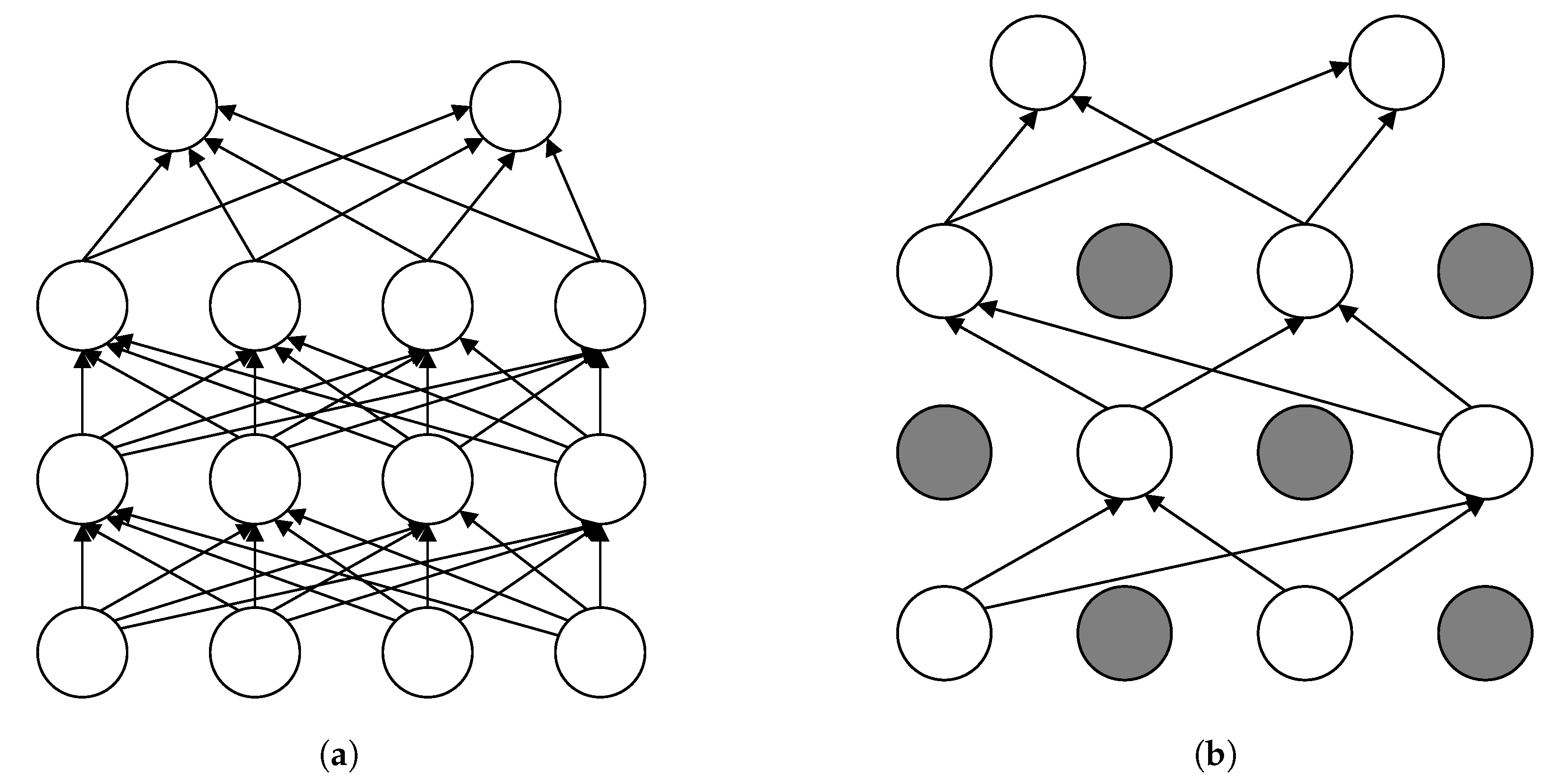
Figure 1. Dropout neural network model: (a) standard neural network; and (b) neural network with dropout.
Energies 12 00995 g001
Figure 2. The instantiation model of DADDNN.
Energies 12 00995 g002
Figure 3. Learning rate curve.
Energies 12 00995 g003
Figure 4. Relationship between network loss and training epoch.
Energies 12 00995 g004
Figure 5. Relationship between network loss and training iteration.
Energies 12 00995 g005
Figure 6. Relationship between network loss and learning rate.
Energies 12 00995 g006
Figure 7. Performance comparison of different network structures.
Energies 12 00995 g007
Figure 8. Performance comparison of different activation functions.
Energies 12 00995 g008
Figure 9. Training loss of different optimization algorithms: (a) integral convergence comparison; and (b) initial training loss.
Energies 12 00995 g009
Figure 10. Classification results of different optimization algorithms: (a) classification accuracy of different optimization algorithms; and (b) Auc@Roc of different optimization algorithms.
Energies 12 00995 g010
Figure 11. Convergence process of DADDNN without dropout: (a) network loss; and (b) diagnosis accuracy.
Energies 12 00995 g011
Figure 12. Convergence process of DADDNN with dropout: (a) network loss; and (b) diagnosis accuracy.
Energies 12 00995 g012
Table 1. Samples distribution of different datasets.
Category SamplesDataset 1Dataset 2Dataset 3Total Dataset
PD1102031
LD132368104
HD3245128205
LT701724
MT2204769
MLT0104454
HT5014157221
NC0265278
Total135118533786
Table 2. Diagnosis accuracies of various methods under different datasets (%).
DatasetIEC 60599Duval TriangleSAEDBNGSSVMDADDNN
Dataset 157.666.782.977.182.993.9
Dataset 248.365.571.467.982.192.9
Dataset 342.148.163.259.462.475.2
Total dataset42.660.066.362.270.380.5
Average accuracy47.760.171.066.774.485.6
Table 3. Diagnosis accuracy of each fault category in Total dataset (%).
CategoryIEC 60599Duval TriangleSAEDBNGSSVMDADDNN
PD100.00.087.50.087.587.5
LD30.861.511.569.246.257.7
HD23.568.688.272.582.490.2
LT16.750.016.716.716.750.0
MT76.541.270.670.670.682.4
MLT0.00.015.40.015.453.8
HT72.796.487.378.285.590.9
NC0.00.063.257.957.957.9
Table 4. Standard data sets information based UCI.
Data SetClassAttributesInstancesTrain SamplesTest Samples
Breast cancer230569469100
Iris3415012030
Wine31317814236
Class identification6921417143
Table 5. Analysis results of model performance with standard datasets.
Data SetModelStructureActivation
Function
AlgorithmTrain
Accuracy (%)
Test
Accuracy (%)
Breast cancerDNN6 layers
600 units
TanhSGD92.593.9
DNN6 layers
600 units
TanhSGD+Momentum93.293.9
DNN6 layers
600 units
TanhAdagrad94.996.0
DNN6 layers
600 units
TanhDynamic Adam96.097.0
IrisDNN5 layers
500 units
ReluSGD98.3100.0
DNN5 layers
500 units
ReluSGD+Momentum99.2100.0
DNN5 layers
500 units
ReluAdagrad99.2100.0
DNN5 layers
500 units
ReluDynamic Adam99.2100.0
WineDNN6 layers
600 units
TanhSGD67.072.2
DNN6 layers
600 units
TanhSGD+Momentum69.088.9
DNN6 layers
600 units
TanhAdagrad95.1100.0
DNN6 layers
600 units
TanhDynamic Adam97.2100.0
Glass identificationDNN6 layers
600 units
TanhSGD35.744.2
DNN6 layers
600 units
TanhSGD+Momentum35.738.9
DNN6 layers
600 units
TanhAdagrad74.872.7
DNN6 layers
600 units
TanhDynamic Adam83.681.4