Multi-Pattern Data Mining and Recognition of Primary Electric Appliances from Single Non-Intrusive Load Monitoring Data

Abstract

The electric power industry is an essential part of the energy industry as it strengthens the monitoring and control management of household electricity for the construction of an economic power system. In this paper, a non-intrusive affinity propagation (AP) clustering algorithm is improved according to the factor graph model and the belief propagation theory. The energy data of non-intrusive monitoring consists of the actual energy consumption data of each electronic appliance. The experimental results show that this improved algorithm identifies the basic and combined class of home appliances. According to the possibility of conversion between different classes, the combination of classes is broken down into different basic classes. This method provides the basis for power management companies to allocate electricity scientifically and rationally.

1. Introduction

In the past few decades, electrical energy has developed rapidly, and a substantial investment has been made towards the construction of intelligent metering power grids [1]. Power management enterprises pay more and more attention to the reliability and quality of electric energy. Therefore, rational allocation of energy and reduction of energy consumption are the top priority of power management enterprises. The energy consumption of household electricity takes up a significant part of energy consumption. Intelligent monitoring of household electricity is an essential prerequisite for improving energy efficiency, which is significant for building a safe and economic power system [2,3]. High-level intelligent power network should deal with various load demands automatically, and can be controlled according to different emergencies, as shown in Figure 1. Based on advanced computer science and technology, combined with cloud processing and machine learning algorithms, power companies expect to build an automated, efficient and energy-saving smart grid. There are two main ways to identify the power levels of various electrical appliances. The first method is intrusive load monitoring, which is a method of recording the operation status of each appliance and requires installing electricity meters on each household appliance. In practical application, this method has complex circuit modification and high installation cost. The second method is non-intrusive load monitoring (NILM), which denotes the class of methods and algorithms able to perform this task by using the electrical parameters measured at a single point [4,5]. The smart meter at the entrance of the home circuit records the data characteristics of power, voltage and current. By decomposing the monitoring load data, we can identify the rated power of different electrical appliances. The power company can obtain the usual information about the user’s electricity, to make a scientific and reasonable decision. This method can reduce the cost of installation and reduce the level of interference in measurement [6]. Commonly used clustering methods for identifying appliances include the following: Hart first proposed non-intrusive household appliance load monitoring and analyzed the algorithm and characteristics, in this case, the essence of this method is to decompose the aggregated load data of household appliance [7]. After decades of research, many methods have been applied to pattern recognition of NILM. Some representative methods are K-means, K-nearest neighbor, enhanced ISODATA and artificial neural network [8,9,10,11]. These methods provide some ideas for identifying the operating mode of electrical appliances, but when there is a large number of home appliances, the recognition results are often not ideal. Frey and Dueck first proposed a standard AP clustering algorithm to solve the clustering problem [12]. The standard AP clustering algorithm can be derived from the factor graph model and the belief propagation theory [12,13]. The factor graph model, proposed by Kschischang and Frey, is a graph description method where the global function is decomposed into the product of the local function [14]. The theory of belief propagation was proposed by Pearl and is a kind of message transfer algorithm for inference in the graph model [15]. Since its publication, AP clustering algorithm has been applied in many fields because of its unique clustering characteristics.

In this paper, we first discuss a method of preprocessing large monitored power data where the noise and mutation was deleted. Then we introduced an improved AP clustering algorithm, where the difficulty of electrical identification was overcome by redefining the similarity matrix S of the AP clustering algorithm and adding two new messages. To analyse the operation rule of electrical appliances, we define the power of a single electrical appliance as a basic class and define the sum of the operating power of two or more electrical appliances as a combination class. We then analyzed and discussed the experimental results and distinguished between the basic and combined classes according to the difference method, and we demonstrated how the combined class was decomposed into the basic class. Finally, we concluded that through the improved AP clustering algorithm, the basic and combined classes could be identified, providing a new method for identifying household appliances.

2. Data Preprocessing

We monitored the electricity consumption of a family and obtained the data set used in this work. The electric meter measures the overall operation of 12 electrical appliances. The meter recorded the power consumed by the family every minute for February 2011, and a total of 40,320 data points (=60 min × 24 h × 28 d) were recorded for the entire month. The time in a cycle (from one idle time period to the next idle time period) was divided into four segments: startup, stable operation, shutdown, and idle time [10], as shown in Figure 2.

The power consumed is unstable for a short time due to the sudden start-up or shut down of electrical appliances. Figure 3 shows the monitoring data for the entirety of 8 February 2011, and each point in the figure represents aggregated load per minute. Peaks were observed in the data during the morning and afternoon, whereas data was more stable during the night. Therefore, the monitoring data of the electric meter was identified by a piecewise method, and the data was preprocessed as follows:

(1)

During idle time: there is no electrical work, the monitoring power value is close to 0 (<10 W), so it is set to 0.

(2)

During stable operation: due to the interference of external factors, there were random abrupt data. These mutation data was replaced by the average value of the time monitoring data. If the difference between three or more continuous monitoring values did not exceed 5% of their average value, we considered that this time was in a stable operation stage. In the study, the data in the stable stage were used for calculation.

(3)

The daily data was divided into three parts according to the family’s daily habits: morning (06:00–14:00), afternoon (14:00–22:00), and night (22:00–06:00).

In the monitoring process, if an electrical appliance is turned on or off, the power data will be transferred from one level to another, and each level corresponds to a power class. The monitoring data is not stable during the startup and shutdown periods, so it is not suitable to be used as valid data. The stable operation phase is the most important of the four segments because it is crucial for identifying the power class of the electrical appliances.

3. Methodology

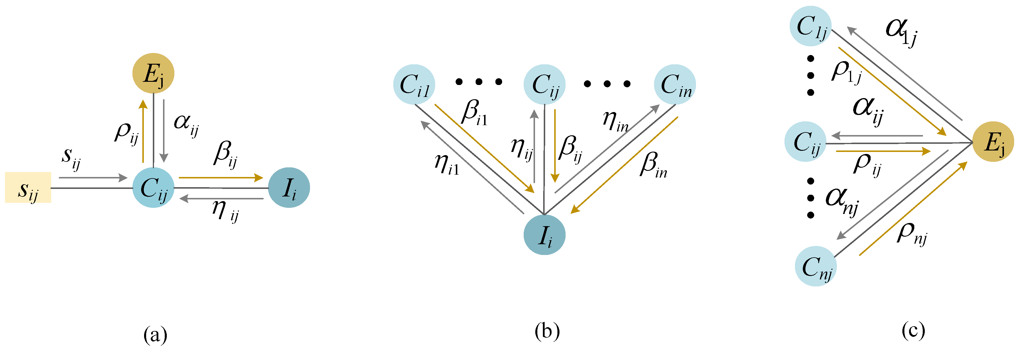
3.1. Standard AP Clustering Algorithm

The model assumes that there are n variable nodes and m function nodes, in which the n variable nodes corresponding to the n random variable C = {c₁, c₂, …, c_n}, and the m function nodes corresponding to the m functions Φ = {φ₁, φ₂, ..., φ_m}. Dueck proposed the Max-Product BP rule. According to which the message from variable node c_i to function node φ_l is equal to the product of message from other function nodes to c_i node. The message from function node φ_l to variable node c_i is the edge function of the product of message from φ_l and other variable nodes to φ_l node relative to c_i. The messages ${\mu }_{c_i\to {\phi }_l}(c_i)$ that the variable node c_i passes to the function node φ_l could be expressed as [16,17]:

$${\mu }_{c_i\to {\phi }_l}(c_i)={\displaystyle \sum _{\left\{l^{\prime }\right|{\phi }_{l^{\prime }}\in {\phi }_{(ne(c_i)\backslash l)}\}}{\mu }_{{\phi }_{l^{\prime }}\to c_i}(c_i)}$$

(1)

where ne(c_i) represents the set of index numbers for all c_i, ne(c_i)\l means removing l from the index number of ne(c_i); $\left\{l^{\prime }\right|{\phi }_{l^{\prime }}\in {\phi }_{(ne(c_i)\backslash l)}\}$ means that the set of remaining index numbers with φ_l is removed from φ; The messages ${\mu }_{{\phi }_l\to c_i}(c_i)$ that the function node φ_l pass to the variable node c_i can be expressed as:

$${\mu }_{{\phi }_l\to c_i}(c_i)=\max {\phi }_l(c_{ne({\phi }_l)}\backslash c_i)+{\displaystyle {\sum }_{\left\{i^{\prime }\right|c_{i^{\prime }}\in c_{ne({\phi }_l)}\backslash c_i\}}{\mu }_{c_{i^{\prime }}\to {\phi }_l}(c_i)}$$

(2)

where φ_l(c_ne(φ_l)\c_i) represents the set of φ_l that removes φ_l(c_i); $\left\{i^{\prime }\right|c_{i^{\prime }}\in c_{ne({\phi }_l)}\backslash c_i\}$ means that the set of remaining index numbers with c_i is removed from c; ${\mu }_{c_{i^{\prime }}\to {\phi }_l}(c_i)$ represents the message passed from the variable node c_i to the function node φ_l. In this paper, the improved AP clustering algorithm utilized the Max-product BP rule operation.

3.2. Improved AP Clustering Algorithm

3.2.1. Challenges with Standard AP Clustering Algorithm

Figure 4 shows a typical factor graph model of the AP clustering algorithm. The message transfer model in Figure 4 is shown in Figure 5. The standard AP clustering algorithm consists of the similarity matrix S = {s_ij}, the attraction message matrix R = {ρ_ij}, and the ownership message matrix A = {α_ij} (i, j = 1, 2, …, n). The data point is recorded as X = {x₁, x₂, ..., x_n}, and two kinds of message ρ_ij and a_ij are alternately updated in the AP clustering algorithm. In Figure 4 and Figure 5, E and I are function node matrices, α, β, η, ρ and s are messages between variable nodes and function nodes. In standard AP clustering algorithm and improved AP clustering algorithm, these functions and messages follow the same calculation rules.

By loosening the constraints of AP clustering algorithm, Leone et al. proposed a soft constrained AP clustering algorithm [18]. After that, Leone et al. introduced a semi-supervised idea and proposed a semi-supervised soft constrained AP clustering algorithm [19]. Givoni and Frey considered that two points must belong to the same class or do not belong to the same class in an instance constraint, and then they proposed a semi-supervised AP clustering algorithm model based on instance constraints [20].

The advantage of the AP clustering algorithm is to exchange message in iteration to approach the optimal result. However, it also has two following shortcomings in the identification of electrical patterns. (1) The computational complexity of the algorithm is relatively large because the message is passed between each data point. For N points, each point needs to transmit (N − 1) messages to other nodes, resulting in the need to compute N × (N − 1) messages in each iteration, which is almost impossible for a large number of data to be completed in an acceptable time. (2) For power data, because the number of members of different classes varies greatly, a large class may be divided into several sub-classes during the clustering process, which leads to high similarity among sub-classes. The reason for this is that many of the same values are potential category centers, each point receives information from all other points, although one point has become a category center, it does not guarantee that another point with the same value will not become the center of the other category. Therefore, an improved AP clustering algorithm based on the factor graph model and the belief propagation theory is proposed to solve those two problems. The improved AP clustering algorithm not only reduced the amount of computation in the operation process, but it also merged highly similar categories while reserving the excellent clustering performance of conventional AP clustering algorithms.

3.2.2. Improvement Measures

To overcome the adverse effects of the AP algorithm, we have improved the standard AP clustering algorithm in two aspects. On the one hand, we redefine the similarity matrix and record the number of times and its value for the point with the same value. The aim is to avoid the same value as the central point of multiple categories. Through the new similarity matrix S, the amount of computing in the AP clustering algorithm is no longer determined by the total number of samples, but by the number of samples with different values. On the other hand, we have added new function nodes and new delivery message. The purpose of this is to integrate other categories within the neighborhood of a point when it has become the central point of the category. Therefore, when a point has become a class center, the message it transmits can be divided into two categories: in its neighborhood and out of the area. In its area, it passes a negative infinity value to other points, which makes other points in the area impossible to become the central points of the category. Outside its neighborhood, it passes a message with a value of 0 to other points, without affecting the point outside the field to become the central point of the category.

The issue of sizeable computational complexity occurs because there are many data points with the same power value in the sample electric power data. In order to reduce the computation time between the same data points, we redefined the similarity matrix S, S = {s_ij(c_ij)}, where s_ij represents the similarity between the data point x_i and the data point x_j, and the s_ij is defined as the following in the improved AP clustering algorithm, as shown in Equation (3):

$$s_{ij}=\{\begin{array}{ll}-h_i\left|x_i-x_j\right|& i\ne jand{c}_{ij}=1.\\ 0& i\ne jand{c}_{ij}=0.\\ p& i=j.\end{array}$$

(3)

where p is the reference degree of the similarity matrix S, which is generally the minimum, average, or maximum value of the matrix S; x is the data point, and h_i is the number of x_i. c_ij represents a variable node whose value is 0 or 1.

To solve the second issue, a new H (c₁₁, ..., c_ii, ..., c_nn) function node was added to the factor graph model of the AP clustering algorithm, and the H function node was connected with all diagonal variable nodes of the C matrix. The function node H and the variable node C transferred the message types ω and δ. The new AP factor diagram model was shown in Figure 6, and the new message transfer model was shown in Figure 7.

The two-value variable node matrix C consists of c_ij, c_ij = 0 or 1. If c_ij = 0, the data point x_i does not select the data point x_j as its category representative point. If c_ij = 1, the data point x_i selects the data point x_j as its category representative point. The clustering criterion function F is as follows:

$$F(S,I,E)={\displaystyle {\sum }_{i\in \{1,2,\dots ,n\}}{\displaystyle {\sum }_{j\in \{1,2,\dots ,n\}\backslash i}{s}_{ij}}+}{\displaystyle {\sum }_{i\in \{1,2,\dots ,n\}}{I}_i}+{\displaystyle {\sum }_{j\in \{1,2,\dots ,n\}}{E}_j}$$

(4)

where I is the uniqueness constraints function node matrix I = {I_i (c_i1, c_i2, …, c_ij, …, c_in)}; E is a node matrix of the existence constraint function where E = {E_j (c_1j, c_2j, …, c_ij, …, c_nj)} (j = 1, 2, ..., n):

$$I_i(c_{i1},c_{i2},\dots ,c_{ij},\dots ,c_{in})=\{\begin{array}{ll}-\infty & if{\displaystyle {\sum }_{j=1}^n{c}_{ij}\ne 1.}\\ 0& otherwise.\end{array}(i=1,2,\dots ,n)$$

(5)

$$E_j(c_{1j},c_{2j},\dots ,c_{ij},\dots ,c_{nj})=\{\begin{array}{ll}-\infty & if{c}_{jj}=0but\exists i:c_{ij}=1.\\ 0& otherwise.\end{array}$$

(6)

The I function node matrix guarantees that every data point only has one category representative point. The E_j function node matrix guarantees that if the data point x_i selects the data point x_j as its category representative point, x_j must also choose its own as the category representative point, otherwise it will make the clustering criterion function fail to get the maximum value.

Two classes of sets G_i and V_i are defined before defining the form of the H function, such as Equations (7) and (8), and the H function node is defined as Equation (9):

$$G_i=\left\{j|\frac{\left|x_i-x_j\right|}{\left|x_i+x_j\right|}\le 0.05,j=1,2,\dots ,nbutj\ne i\right\}.(i=1,2,\dots ,n)$$

(7)

$$V_i=\left\{j|{\alpha }_{jj}+{\rho }_{jj}>0,j\in G_i\right\}.(i=1,2,\dots ,n)$$

(8)

$$H(c_{11},\dots ,c_{ii},\dots ,c_{nn})=\{\begin{array}{ll}\infty & c_{ii}=0and{V}_i\ne \varphi .\\ 0& otherwise.\end{array}$$

(9)

where α and ρ are messages passed between nodes. As shown in Figure 7, s, α, η, and ω are the messages that the function node passes to the variable node, and ρ, β, δ are the messages that the variable node moves into the function node. These message transfer procedures follow the binary operation rules, and the binary operation rules are as follows:

$$\mu =\mu (c_{ij}=1)-\mu (c_{ij}=0)$$

(10)

where μ (c_ij = 1) and μ (c_ij = 0) calculation processes follow the Max-product BP rules, according to the Equation (1) variable node message passed to the function ρ_ij and β_ij calculation results are as follows.

$${\rho }_{ij}={\rho }_{ij}(c_{ij}=1)-{\rho }_{ij}(c_{ij}=0)=\left[s_{ij}(c_{ij}=1)+{\eta }_{ij}(c_{ij}=1)\right]-\left[s_{ij}(c_{ij}=0)+{\eta }_{ij}(c_{ij}=0)\right]=s_{ij}+{\eta }_{ij}$$

(11)

$${\beta }_{ij}={\beta }_{ij}(c_{ij}=1)-{\beta }_{ij}(c_{ij}=0)=\left[s_{ij}(c_{ij}=1)+{\alpha }_{ij}(c_{ij}=1)\right]-\left[s_{ij}(c_{ij}=0)+{\alpha }_{ij}(c_{ij}=0)\right]=s_{ij}+{\alpha }_{ij}$$

(12)

According to Equation (2), the message passed from the function node to variable node is calculated as follows:

$${\eta }_{ij}={\eta }_{ij}(c_{ij}=1)-{\eta }_{ij}(c_{ij}=0)={\displaystyle {\sum }_{t:t\ne j}{\beta }_{it}(c_{ij}=0)}-\underset{k:k\ne j}{\max }\left[{\beta }_{ik}(1)+{\displaystyle {\sum }_{t:t\notin \{k,j\}}{\beta }_{it}(0)}\right]=-\underset{k\ne j}{\max }{\beta }_{ik}$$

(13)

In the same way, the message α_ij and ω_i of the function node to be passed to the variable node is as follows:

$${\alpha }_{ij}=\{\begin{array}{ll}{\displaystyle {\sum }_{k:k\ne j}\max [{\rho }_{kj},0]}& i=j.\\ \min \{0,{\rho }_{jj}+{\displaystyle {\sum }_{k\notin \{i,j\}}\max [{\rho }_{kj},0]}\}& i\ne j.\end{array}$$

(14)

$${\omega }_i=\{\begin{array}{ll}-\infty & if{c}_{ii}=0and{V}_i\ne \varphi .\\ 0& otherwise.\end{array}$$

(15)

As shown in Equation (15), the value of message ω is independent of the value of message δ, and message δ does not participate in the iterative process. Using this method, when a data point is a representative point, there is not be a category representative point near it, so that the high similarity category is suppressed. Solving Equations (11)–(15) together can get Equation (16). To prevent the vibration and speed of convergence in the process of message transmission, damping factor λ (generally set to 0.9) was added [21]:

$$\{\begin{array}{l}{\omega }_i=\{\begin{array}{ll}-\infty ,& if{c}_{ii}=0and{V}_i\ne \varnothing ;\\ 0,& otherwise.\end{array}\\ {\rho }_{ij}=\{\begin{array}{l}{s}_{ij}-\underset{k:k\ne j}{\max }[s_{ik}+{\alpha }_{ik}],i\ne j;\\ s_{ii}+{\omega }_i-\underset{k:k\ne j}{\max }[s_{ik}+{\alpha }_{ik}],i=j.\end{array}\\ {\alpha }_{ij}=\{\begin{array}{l}\min \{0,{\rho }_{jj}+{\displaystyle \sum _{k:k\notin \{i,j\}}\max [{\rho }_{kj},0]}\},i\ne j;\\ {\displaystyle \sum _{k:k\ne i}\max [{\rho }_{ki},0],i=j}\end{array}\\ {\rho }_{ij}^u\leftarrow \lambda {\rho }_{ij}^u+(1-\lambda ){\rho }_{ij}^{u-1}\\ {\alpha }_{ij}^u\leftarrow \lambda {\alpha }_{ij}^u+(1-\lambda ){\alpha }_{ij}^{u-1}\end{array}$$

(16)

where ρ^u and α^u are the u iteration, α and ρ are interrelated and need to be iterated until convergence. The category representation point set is Z = {x_i | ρ_ii + α_ii > 0}. With the newly added ω message, the high similarity category can be effectively suppressed. Meanwhile, the excellent clustering performance of the AP clustering algorithm is retained.

3.3. Electrical Appliances Pattern Recognition Process

Household appliances are usually operated at several power levels of the same size. In the long-term monitoring, these power values will appear frequently, thus clustering into different categories. Cluster analysis is a kind of unsupervised learning and is a method of exploring data structure [22]. Each data value in the improved AP algorithm is a potential class representative point, so low-power data can be identified even if the data set contains high-power data. This is the basis for the improved AP clustering algorithm to identify small power classes. According to the living habits of the ordinary family, the user sleeps at night, the number of household appliances is relatively tiny, and the meter measurement data is stable. Electrical appliances are used more frequently after getting up in the morning and after returning home in the afternoon, so there will be a power peak in the morning and the afternoon. To avoid the power peak time is too short to identify the high-power class, so the daily monitoring data is divided into three periods for analysis. The detailed steps of the algorithm were as follows:

(1)

The dataset was inputted with N points {x_i, i = 1, 2, ..., N}, then divided into three periods of time.

(2)

During idle time, the monitored power data was close to 0. It was set to 0. In a stable time, the abrupt value is replaced by the mean value in this period.

(3)

The initial parameters were set as follows: the value of the reference degree p of the similarity matrix S was the opposite number of the maximum value of the dataset, the damping factor λ equaled 0.9, and the number of iterations was set to 200. The initial value of the attraction message matrix R and the ownership message matrix A was set to 0.

(4)

The values of the attraction message matrix R and the ownership message matrix A were calculated according to Equation (16).

(5)

The convergence of matrices A and R was determined. If they did not converge, we advanced to step (6); otherwise we advanced to step (7).

(6)

It was judged whether to reach the number of iterations. If so, we returned to step (3) and reset the initial parameters; if not, we went back to step (4).

(7)

The value of the diagonal of matrix A + R was determined to be higher than or less than 0. If it was greater, the point was a class-representative data point; if it was less, the point was a common data point.

(8)

The category of the measure was determined according to the similarity (Euclidean distance) between the common point and the class-representative point.

The flowchart of the improved AP clustering algorithm is shown in Figure 8. The integration of automatic pattern recognition of electrical appliances is conducive to the rational allocation of power resources. The process of automatic pattern recognition for electric appliances on big monitored data is shown in Figure 9.

4. Analysis and Discussion

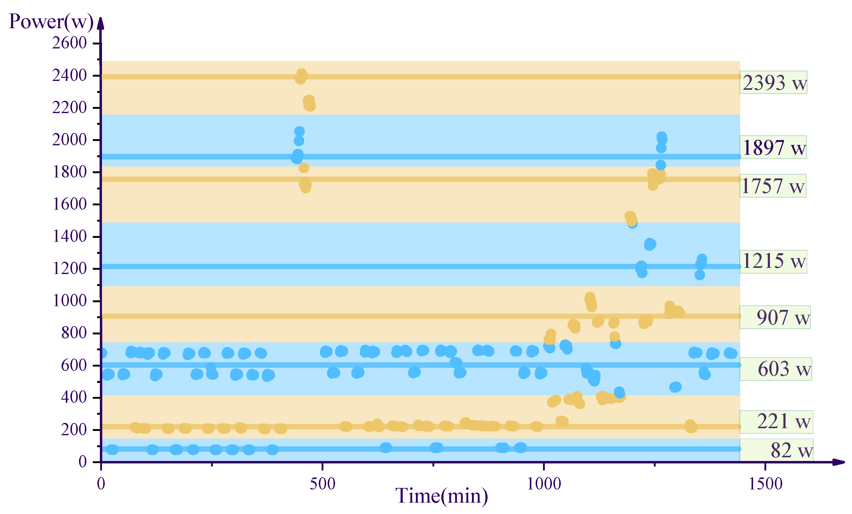
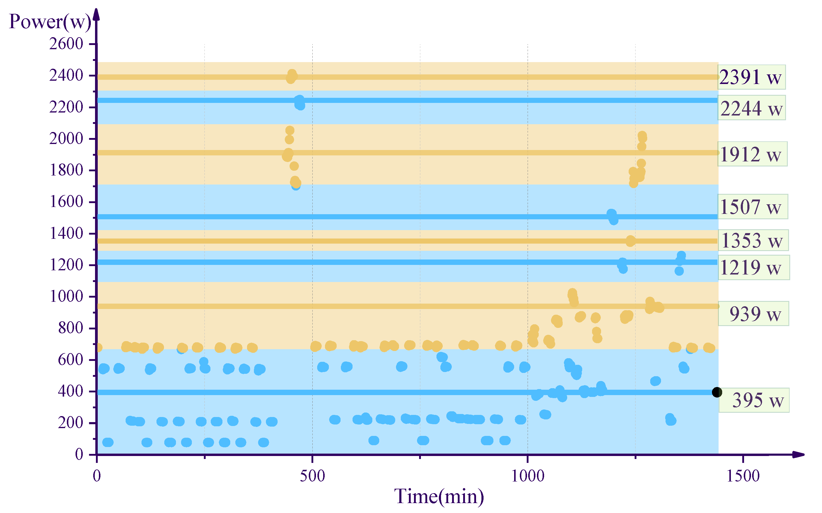
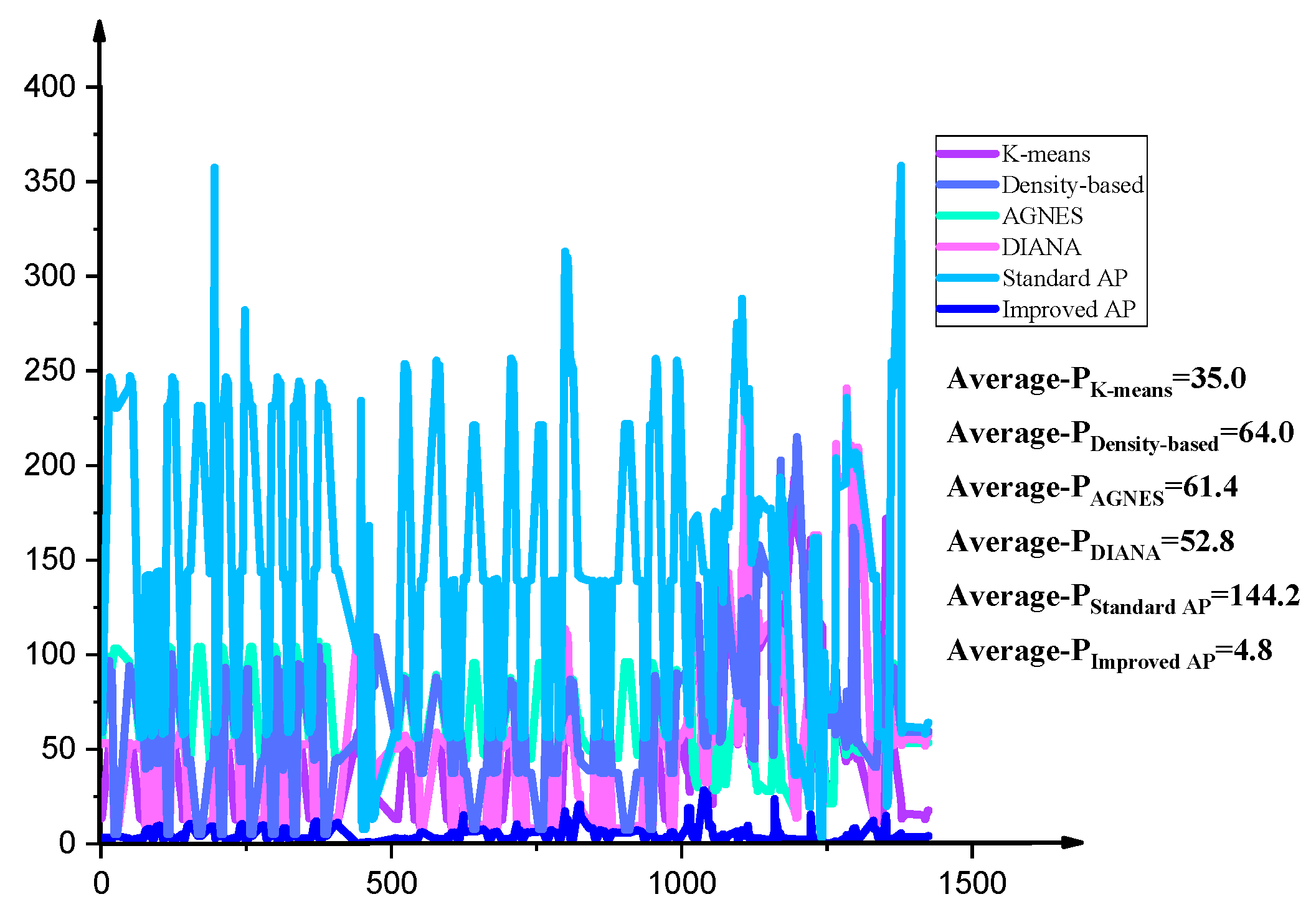
4.1. Comparison of Different Algorithms

To test the improved AP clustering algorithm, 1440 data points from 8 February 2011, were selected for testing and analysis. Six clustering methods such as k-means algorithm, density-based algorithm, hierarchical clustering (agglomerative nesting and divisive analysis), standard AP clustering algorithm, and improved AP clustering algorithm were used to cluster analysis. The k-means algorithm is a classical and extensive clustering method, which can be used to explore data structure [23]. The density-based algorithm is a method of high-density connected regions that is insensitive to noise and can find classes of arbitrary shapes [24]. Hierarchical clustering algorithm can be divided into two types: Agglomerative Nesting (AGNES) and Divisive Analysis (DIANA). In this paper, AGNES and DIANA were chosen as the contrast algorithm [25]. To make these methods have contrast, the improved AP clustering algorithm was used to determine the number of categories, and then the same k value was used for the k-means algorithm and hierarchical clustering. In the density-based algorithm, the neighborhood radius eps = 50 and the minimum neighborhood elements in the neighborhood were minPts = 8. In the standard AP clustering algorithm, the p-value took the average of the similarity degree matrix S, the damping factor λ equaled 0.9, and the number of iterations was set to 200. In the improved AP clustering algorithm, the value of p took the opposite number of the maximum value of the data point, the damping factor λ equaled 0.9, and the number of iterations was set to 200. The settings of these initial parameters ensured the final iteration convergence. The clustering results of the six algorithms are shown in

Table 1. The results of different clustering algorithms.

k-Means Algorithm (W)	Density-Based Algorithm (W)	AGNES (W)	DIANA(W)	Standard AP Algorithm (W)	Improved AP Algorithm (W)
82	82	181	82	395	89
222	221	400	221	939	223
503	603	637	506	939	391
687	907	907	736	1219	551
907	1215	1258	1215	1353	688
1335	1757	1510	1353	1353	878
1760	1897	1754	1510	1507	1504
1942	2393	1927	1816	1912	1757
2233	-	2233	2233	2244	1951
2393	-	2393	2392	2391	2224

. The results of k-means algorithm, Density-based algorithm, AGNES and DIANA algorithms in the Table 1 are the mean values. The results of standard AP and improved AP algorithms are determined by Z = {x_i | ρ_ii + α_ii > 0}. The comparison of the recognition ability of the six algorithms is shown in

Table 2. Comparison of six algorithms’ recognition ability.

Electric Appliances (Rated Power)	K-Means Algorithm	Density Based Algorithm	AGNES	DIANA	Standard AP Algorithm	Improved AP Algorithm
Plasma TV (220 W)	√ (0.9%)	√ (0.5%)	× (17.7%)	√ (0.5%)	/	√ (1.4%)
Frig (400 W)	/	/	√ (0.0%)	/	√ (1.3%)	√ (2.25%)
Furnace (550 W)	× (8.5%)	× (9.6%)	× (15.8%)	× (8.0%)	/	√ (0.2%)
Oven (900 W)	√ (0.8%)	√ (0.8%)	√ (0.8%)	× (18.2%)	√ (4.3%)	√ (2.4%)
Bath (1500 W)	× (11.0%)	× (19.0%)	√ (0.7%)	√ (0.7%)	√ (0.5%)	√ (0.3%)
Dryer-p1 (1800 W)	√ (2.2%)	√ (2.4%)	√ (2.6%)	√ (0.9%)	/	√ (2.3%)
Microwave (2000 W)	√ (2.9%)	× (5.2%)	√ (3.7%)	/	√ (4.4%)	√ (2.5%)
Dryer-p2 (2200 W)	√ (1.5%)	× (8.8%)	√ (1.5%)	√ (1.5%)	√ (2.0%)	√ (1.1%)

* Notes: (*%) is the value of relative error. “√” means that the relative error is less than 5%, “×” means that the relative error is more than 5%, and “/” means that the algorithm does not recognize the electrical power.

. If the relative error (=(|calculated value-rated power|)/(rated power)) is less than 5%, the recognition result is considered correct. The clustering results are shown in Figure 10, Figure 11, Figure 12, Figure 13, Figure 14 and Figure 15.

It is evident from Table 1 that the standard AP clustering algorithm will divide the small numerical power data into the 395 W class. The same category representation points repeat, such as the two categories of 939 W and 1353 W. During the test, it was found that as the data volume increases, this phenomenon becomes more significant. Sometimes there were many new categories of representative points near the category-representative points, which affected the final judgment. Table 2 shows that the improved AP clustering algorithm can recognize the whole classes of electric appliances on the day. k-means clustering algorithm, the hierarchical clustering algorithm, and standard AP clustering algorithm hardly recognized low-power appliances. The density-based clustering algorithm was weak in identifying the high-power appliances.

As seen in Figure 10, Figure 11, Figure 12, Figure 13, Figure 14 and Figure 15, to compare the clustering effects of the six clustering algorithms, we use the same stripe to represent the same class to express the clustering results. The result of the k-means calculation was influenced by the initial random values, causing the final results to be inconsistent and unable to make a correct and reasonable decision. The improved AP clustering algorithm identified small power data and did not display similar category-representative points near the class-representative points, and each test result was stable. As shown in Table 2, the five algorithms k-means, the density-based algorithm, AGNES, DIANA and the standard AP clustering algorithm have the problem that some electrical appliances cannot recognize or recognize errors. Only the improved AP clustering algorithm can recognize all electrical appliances. We choose the cohesion index to evaluate the clustering performance of different algorithms objectively, as seen in Figure 16. We calculate the average distance Pi from each data point to all points of its class, and then average all Pi values of each algorithm to get the final average-P of each algorithm. It can be seen from the graph that the average-P (4.8) of the improved AP clustering algorithm is the minimum value. The results show that the improved AP clustering algorithm can make each point gather near the representation point of the category and the clustering performance is the best.

4.2. Experimental Result

To identify the basic class and combined class of all the power of household electrical appliances, 40320 monthly data points X = {x₁, x₂, ..., x₄₀₃₂₀} monitored by household total electricity meter were processed among three time periods. Before recognizing the electrical pattern, we preprocessed the data according to the method in Section 2 and selected the data in stable operation stage for clustering analysis. The improved AP clustering algorithm was used to cluster analysis according to Equation (16). The initial parameters in the three time periods of this experiment were set as follows: p = −max {x₁, x₂, ..., x_n}, damping factor λ = 0.9, and iteration of 200. The setting of the initial parameter ensured the convergence of the algorithm in the iteration.

Table 3. Identification results of electric power classes.

Class	Morning (W)	Afternoon (W)	Night (W)	Average (W)
C1	75	76	77	76
C2	94	-	-	94
C3	122	129	129	127
C4	141	150	-	146
C5	186	-	-	186
C6	213	201	206	207
C7	-	223	230	226
C8	251	252	262	255
C9	306	288	293	296
C10	-	326	-	326
C11	360	380	356	365
C12	433	427	428	429
C13	479	479	-	479
C14	538	554	532	541
C15	615	622	614	617
C16	719	688	716	708
C17	-	762	795	778
C18	842	-	-	842
C19	-	900	901	900
C20	978	1008	-	993
C21	1092	1160	1092	1115
C22	1223	-	1233	1228
C23	-	1343	-	1343
C24	1482	1515	1435	1477
C25	-	1693	-	1693
C26	1858	1990	-	1924
C27	-	-	2108	2108
C28	2259	-	-	2259
C29	-	2349	-	2349
C30	-	2712	-	2712

shows the recognition results of the three time periods and their comprehensive results. The results include basic class and combined class. In the next section, we distinguish the basic class and combined class, and divide the combined class into several basic class according to the maximum probability.

4.3. Power Load Decomposition

The purpose of power load decomposition is to decompose the aggregated power load into multiple single electrical loads [26]. Arberet et al. extracted the single equipment signal from the aggregated load curve of a family, synthesized the operation of the single equipment into the total signal, and compared the synthetic signal with the real signal [27]. As demonstrated in the previous section, the improved AP clustering algorithm was able to identify the basic and combined classes of the electrical appliances. However, it is not possible to differentiate between the basic and combined classes as they are presented in Table 3. Based on real-life experience and monitoring data from total household electricity consumption, it can be seen that power shifts from one stable operation stage to another, and the conversion time is relatively short. Usually, the conversion process is completed in 1~5 min. In most cases, only one electrical switch state has changed in such a period. During the calculation of the monitoring data in two adjacent stable operation stages, the values reflected in the two stable stages in the running state of a household appliance is different. The difference between the values is the basic class, as shown in Equation (17).

$$B_T=\left|C_T-C_{T-1}\right|$$

(17)

where C_T represents the average power of the T stable operation stage. C_T−1 represents the average power of the (T − 1) stable operation stage. B_T represents the value of the power data monitored from the (T − 1) stage to the T stage. The energy usage of a single household during February 2011 was monitored, from which B_T was determined using Equation (17). All B_T power values were identified by the improved AP clustering algorithm following the steps detailed in Section 4.2. The identification results are presented in

Table 4. Identification results of basic class position.

Class	Morning (W)	Afternoon (W)	Night (W)	Average (W)
B0	-	-	1	1
B1	18	14	13	15
B2		46	-	46
B3 → C1	75	71	67	71
B4 → C4	145	141	135	140
B5 → C10	322	327	324	324
B6 → C13	462	459	467	463
B7 → C15	594	601	594	596
B8 → C18	-	-	810	810
B9 → C20	1003	1012	-	1008
B10 → C21	-	-	1118	1118
B11	-	1567	-	1567
B12 → C25	-	1668	-	1668
B13 → C28	-	2234	-	2234

.

As shown in Table 4, B₀ is 1 W, which was generated by the stable running stage and thus should not be used as a basic class. Moreover, Table 3 shows that all classes were identified aside from B₁, B₂, and B₁₁. This method can distinguish the basic and combined classes in Table 2. It can be seen from the numerical comparison that C₁, C₄, C₁₀, C₁₃, C₁₅, C₁₈, C₂₀, C₂₁, C₂₅, and C₂₈ are the basic classes, and the basic classes should also include B₁, B₂ and B₁₁ in Table 4. Furthermore, the rest of the other classes are combined classes.

Once the basic and combined classes were distinguished, the combined classes needed to be disaggregated into the basic classes. Usually, when a stable running class is switched to another stable running class, only one electrical device’s working condition is changed so that all combination classes can be disaggregated this way. The later stable running class may be the basis for the previous stable combined class. The decomposition process of a combined class can be expressed by the following equation:

$$C_i=C_m+C_n$$

(18)

where C_i is a combined class that needs to be disaggregated. C_m is the most frequent combination or basic class after the C_i class. Since C_i is made up of C_m, the value of C_i should be greater than that of C_m. The corresponding class C_m is counted before each combination of the class C_i is disaggregated. If there are no combined class, the value of C_m is 0. C_n is the basic class. For any combination class that needs to be disaggregated, C_i and C_m are known. By selecting the appropriate C_n base class, any combination of classes can be disaggregated, as shown in

Table 5. Power load disaggregation results.

Combination Class Ci	Combination or Basic Class Cm	Basic Class Cn	Error (W) e = |Ci − Cm − Cn|	Decomposition Results
C2	C1	B1	e2 = |94 − 76 − 15| = 3	C2 = C1 + B1 + e2
C3	C1	B2	e3 = |127 − 76 − 46| = 5	C3 = C1 + B2 + e3
C5	C4	B2	e5 = |186 − 146 − 46| = 6	C5 = C4 + B2 − e5
C6	C1	C4	e6 = |207 − 76 − 146| = 15	C6 = C1 + C4 − e6
C7	C6	B1	e7 = |226 − 207 − 15| = 4	C7 = C1 + C4 + B1 + e7
C8	C3	C4	e8 = |255 − 127 − 146| = 18	C8 = C1 + B2 + C4 − e8
C9	C8	B2	e9 = |296 − 255 − 46| = 5	C9 = C1 + B2 + C4 + B2 − e9
C11	C9	C1	e11 = |365 − 296 − 76| = 7	C11 = C1 + B2 + C4 + B2 + C1 − e11
C12	C11	C1	e12 = |429 − 365 − 76| = 12	C12 = C1 + B2 + C4 + B2 + C1 + C1 − e12
C14	C13	C1	e14 = |541 − 479 − 76| = 14	C14 = C13 + C1 − e14
C16	C6	C13	e16 = |708 − 207 − 479| = 22	C16 = C1 + C4 + C13 + e16
C17	C16	C1	e17 = |778 − 708 − 76| = 6	C17 = C1 + C4 + C13 + C1 − e17
C19	C17	C4	e19 = |900 − 778 − 146| = 24	C19 = C1 + C4 + C13 + C1 + C4 − e19
C22	C6	C20	e22 = |1228 − 207 − 993| = 28	C22 = C1 + C4 + C20 + e22
C23	C21	C4	e23 = |1343 − 1115 − 146| = 82	C23 = C21 + C4 + e23
C24	C23	C4	e24 = |1477 − 1343 − 146| = 12	C24 = C21 + C4 + C4 − e24
C26	C19	C20	e26 = |1924 − 900 − 993| = 31	C26 = C1 + C4 + C13 + C1 + C4 + C20 − e26
C27	C11	C25	e27 = |2108 − 365 − 1693| = 50	C27 = C1 + B2 + C4 + B2 + C1 + C25 + e27
C29	C26	C13	e29 = |2349 − 1924 − 479| = 54	C29 = C1 + C4 + C13 + C1 + C4 + C20 + C13 − e29
C30	C29	C10	e30 = |2712 − 2349 − 326| = 37	C30 = C1 + C4 + C13 + C1 + C4 + C20 + C13 + C10 + e30

.

As shown in Table 5, the maximum error in the disaggregation of a combined class is 82 W, which occurs during the disaggregation of the C₂₃. The value is close to the value of the basic class C₁, which is likely to be the result of the simultaneous conversion of the two basic classes C₄ and C₁. To illustrate basic and combined classed for electrical loads, an example is given here to explain it. We chose a time fragment from the data monitored by the electric energy meter. This time fragment included three running classes, such as C₁, C₆, and C₁₄, as shown in Figure 17. The different column in the Figure 17 represent different electrical class.

The points in the red circle are unstable monitoring data from one class to another, which should be eliminated in the study. The difference of C₆ to C₁ is 137 W, which is approximately equal to the value of the base class C₄ (146 W). It shows that the combined class C₆ is composed of the basic classes C₁ and C₄. From C₁₄ to C₁, the data value of the energy meter was reduced by 460 W, which is approximately equal to the value of the basic class C₁₃ (479 W). It shows that C₁₄ is made up of the basic classes C₁ and C₁₃. In this way, we can identify that C₁, C₄, and C₁₃ are basic classes, and C₆ and C₁₄ are combined classes. All basic classes and combined classes can be identified by this method.

Each combined class is composed of multiple electrical appliances working at the same time. Based on this method, we can find out the combination mode of each combination class. The disaggregation results of all the combined classes are shown in Table 5.

4.4. Discussion

Pattern recognition of electrical appliances is focused on identifying different power levels. It is necessary to ensure that low-power class with more occurrences are not duplicated and that high-power class with fewer occurrences are identified. By redefining the similarity matrix S and adding a new function node H of AP clustering algorithm, the frequency and the value of power can be considered together. By using the improved AP method, 30 basic and combined classes were identified. In Section 4.3, three additional basic classes (15 W, 46 W, 1567 W) can be identified based on the maximum probability method. If the working state of two electrical appliances is completely synchronized, the power of the two electrical appliances will be determined as a basic, instead of combined class. In this study, 20 combined classes were disaggregated into basic classes, of which 19 were successfully disaggregated with small error values. Only one disaggregation of a combined class had an error value of 82 W. Thus, and the value could not be determined as a result of instrument error or the simultaneous change of multiple electrical appliances. In the future, the addition of datasets can help determine the source of error. The improved AP clustering algorithm provides a new method for pattern recognition of NILM. According to this method, the power company can use the data of monitoring equipment to establish a monitoring and forecasting model for household electricity consumption.

5. Conclusions

By developing an improved AP clustering algorithm, this paper studied the problem of pattern recognition for electrical appliances and electrical load decomposition. The improved AP clustering algorithm redefined the similarity matrix, adding new function nodes and two kinds of new messages. It not only reduced the computational complexity of the algorithm but also overcame the deficiencies of the standard AP clustering algorithm. The improved AP clustering algorithm accurately identified the basic and combined classes of electric appliances. According to the cohesion index, the average-P of the improved AP clustering algorithm is only 4.8, which is the smallest among the six algorithms. The value shows that the clustering performance of the improved AP clustering algorithm is better than the other five algorithms. The improved AP clustering algorithm aggregates the most compact classes. This study not only identifies multiple power classes of electrical appliances, but also disaggregates the combined classes into several basic classes according to the maximum probability. In our research, the data set was provided by a family. In future research, we will validate this method on a wider range of data sets and set different parameters for different families to get better results.

References

1. Wang, D.; Yuan, X.M.; Zhang, M.Q. Power-balancing based induction machine model for power system dynamic analysis in electromechanical timescale. Energies 2018, 11, 438. [Google Scholar] [CrossRef]
2. Mahmood, D.; Javaid, N.; Alrajeh, N.; Khan, Z.A.; Qasim, U.; Ahmed, I.; Ilahi, M. Realistic scheduling mechanism for smart homes. Energies 2016, 9, 202. [Google Scholar] [CrossRef]
3. Ahmed, I.S.; Asmaa, H.R.; Khalled, M.A. A data mining-based load forecasting strategy for smart electrical grids. Adv. Eng. Inform. 2016, 3, 422–448. [Google Scholar]
4. Bonfigl, R.; Principi, E.; Fagiani, M.; Severini, M.; Squartini, S.; Piazza, F. Non-intrusive load monitoring by using active and reactive power in additive Factorial Hidden Markov Models. Appl. Energy 2017, 208, 1590–1607. [Google Scholar] [CrossRef]
5. Suman, G.; Mario, B. An error correction framework for sequences resulting from known state-transition models in Non-Intrusive Load Monitoring. Adv. Eng. Inform. 2017, 32, 152–162. [Google Scholar]
6. Bonfigli, R.; Felicetti, A.; Principi, E.; Fagiani, M.; Squartini, S.; Piazza, F. Denoising autoencoders for Non-intrusive load monitoring: Improvements and comparative evaluation. Energy Build. 2018, 158, 1461–1474. [Google Scholar] [CrossRef]
7. Hart, G.W. Nonintrusive appliance load monitoring. Sr. Memb. 1992, 80, 1870–1879. [Google Scholar] [CrossRef]
8. Chui, K.; Tsang, K.; Chung, S.H.; Yeung, L.F. Appliance signature identification solution using k-means clustering. In Proceedings of the 39th Annual Conference of the IEEE Industrial Electronics Society, Vienna, Austria, 10–13 November 2013; pp. 8420–8425. [Google Scholar]
9. Kim, Y.; Kong, S.; Ko, R.; Joo, S.K. Electrical event identification technique for monitoring home appliance load using load signatures. In Proceedings of the IEEE International Conference on Consumer Electronics, Las Vegas, NV, USA, 10–13 January 2014; pp. 296–297. [Google Scholar]
10. Li, M.C.; Han, S.; Shi, J. An enhanced ISODATA algorithm for recognizing multiple electric appliances from the aggregated power consumption dataset. Energy Build. 2017, 140, 305–316. [Google Scholar] [CrossRef]
11. Srinivasan, D.; Ng, W.S.; Liew, A.C. Neural-network-based signature recognition for harmonic source identification. IEEE Trans. Power Deliv. 2006, 21, 398–405. [Google Scholar] [CrossRef]
12. Frey, B.J.; Dueck, D. Clustering by passing messages between data points. Science 2007, 315, 972–976. [Google Scholar] [CrossRef]
13. Givoni, I.E.; Frey, B.J. A binary variable model for affinity propagation. Neural Comput. 2009, 21, 1589–1600. [Google Scholar] [CrossRef]
14. Kschischang, F.R.; Frey, B.J.; Loeliger, H.A. Factor graphs and the Sum-Product algorithm. IEEE Trans. Inf. Theory 2001, 47, 498–519. [Google Scholar] [CrossRef]
15. Pearl, J. Probabilistic reasoning in intelligent systems: Networks of plausible inference. J. Philos. 1991, 88, 434–437. [Google Scholar]
16. Wang, L.; Zhang, Y.; Zhong, S. Typical process discovery based on affinity propagation. J. Adv. Mech. Des. Syst. Manuf. 2016, 10, 1–13. [Google Scholar] [CrossRef]
17. Dueck, D. Affinity Propagation: Clustering Data by Passing Messages; University of Toronto: Toronto, ON, Canada, 2009. [Google Scholar]
18. Leone, M.; Sumedha; Weigt, M. Clustering by soft-constraint affinity propagation: Applications to gene-expression data. Bioinformatics 2007, 23, 1–11. [Google Scholar] [CrossRef]
19. Leone, M.; Sumedha; Weigt, M. Unsupervised and semi-supervised clustering by message passing: Soft-constraint affinity propagation. Phys. Condens. Matter 2008, 66, 1–11. [Google Scholar]
20. Givoni, I.; Frey, B.J. Semi-supervised affinity propagation with Instance-level constraints. In Proceedings of the 12th International Conference on Artificial Intelligence and Statistics, New York, NY, USA, 8–12 June 2009; pp. 161–168. [Google Scholar]
21. Wang, C.D.; Lai, J.H.; Suen, C.Y.; Zhu, J.Y. Multi-Exemplar affinity propagation. IEEE Trans. Pattern Anal. Mach. Intell. 2013, 35, 2223–2237. [Google Scholar] [CrossRef]
22. Rostaminia, R.; Saniei, M.; Vakilian, M.; Mortazavi, S.S. An efficient partial discharge pattern recognition method using texture analysis for transformer defect models. Int. Trans. Electr. Energy Syst. 2018, 28, 1–14. [Google Scholar] [CrossRef]
23. Faria, P.; Spinola, J.; Vale, Z. Reschedule of distributed energy resources by an aggregator for market participation. Energies 2018, 11, 713. [Google Scholar] [CrossRef]
24. Ester, M.; Kriegel, H.P.; Sander, J.; Xu, X.W. A density-based algorithm for discovering clusters in large spatial databases with noise. In Proceedings of the 2nd International Conference on Knowledge Discovery and data Mining, Portland, OR, USA, 2–4 August 1996; pp. 226–231. [Google Scholar]
25. Leuven, K.U.; Zvrich, E.T.H. Application of clustering for the development of retrofit strategies for large building stocks. Adv. Eng. Inform. 2017, 31, 32–47. [Google Scholar] [Green Version]
26. Kolter, J.Z.; Batra, S.; Ng, A.Y. Energy disaggregation via discriminative sparse coding. Adv. Neural Inf. Process. Syst. 2010, 23, 1153–1161. [Google Scholar]
27. Arberet, S.; Hutter, A. Non-intrusive load curve disaggregation using sparse decomposition with a translation-invariant boxcar dictionary. In Proceedings of the IEEE PES Innovative Smart Grid Technologies, Europe, Istanbul, Turkey, 12–15 October 2014; pp. 1–6. [Google Scholar]
Figure 1. Architecture and main components of a smart grid.
Energies 12 00992 g001
Figure 2. Four segments of electrical operation.
Energies 12 00992 g002
Figure 3. Aggregated load of the subject household for 8 February 2011.
Energies 12 00992 g003
Figure 4. The factor graph model of the standard AP clustering algorithm.
Energies 12 00992 g004
Figure 5. Message transfer model of an AP clustering algorithm. (a) Function nodes sij, Ej and Ii to variable nodes Cij; (b) Variable nodes {Ci1, Ci2, …, Cin} to function nodes Ii; (c) Variable nodes {C1j, C2j, …, Cnj} to function nodes Ej.
Energies 12 00992 g005
Figure 6. The factor graph model of improving AP clustering algorithm.
Energies 12 00992 g006
Figure 7. Improved AP clustering algorithm message passing model. (a) Function nodes sij, Ej and Ii to variable nodes Cij (ij); (b) Function nodes sij, Ej, Ii and H to variable nodes Cij (i = j); (c) Variable nodes {Ci1, Ci2, …, Cin} to function nodes Ii; (d) Variable nodes {C1j, C2j, …, Cnj} to function nodes Ej; (e) Variable nodes {C11, C22, …, Cnn} to function nodes H.
Energies 12 00992 g007
Figure 8. Improved AP clustering algorithm flow chart.
Energies 12 00992 g008
Figure 9. Automatic pattern recognition for electric appliances.
Energies 12 00992 g009
Figure 10. The results of k-means algorithm with k = 10.
Energies 12 00992 g010
Figure 11. The results of the density-based algorithm.
Energies 12 00992 g011
Figure 12. The results of Agglomerative Nesting.
Energies 12 00992 g012
Figure 13. The results of Divisive Analysis.
Energies 12 00992 g013
Figure 14. The results of the standard AP clustering algorithm.
Energies 12 00992 g014
Figure 15. The results of the improved AP clustering algorithm.
Energies 12 00992 g015
Figure 16. Clustering performance comparison of different algorithms.
Energies 12 00992 g016
Figure 17. A schematic diagram of the process of combinatorial class disaggregation.
Energies 12 00992 g017