A Novel Social Spider Optimization Algorithm for Large-Scale Economic Load Dispatch Problem

Abstract

The paper develops an improved social spider optimization algorithm (ISSO) for finding optimal solutions of economic load dispatch (ELD) problems. Different ELD problem study cases can bring huge challenges for testing the robustness and effectiveness of the proposed ISSO method since discontinuous objective functions as well as complicated constraints are taken into account. The improved method is different from original social spider optimization algorithm (SSSO) by performing several modifications directly related to three processes of new solution generation. Namely, the proposed method keeps one formula for the first and the second generations and modify them effectively while SSSO has two different formulas for each generation. In the third generation, the proposed method applies a new formula for determining the mating radius of dominant males and females with the intent to expand search space and avoid falling into local zones. The modifications can support the proposed ISSO method find better solutions with faster manner than SSSO while the number of control parameters and the number of computational processes can be reduced. As a result, the proposed method can find much less generation cost and achieve faster search speeds than SSSO for all considered systems. On the other hand, the search ability evaluation of the proposed method is also given by comparing results with other existing methods available in previous studies. The proposed method can obtain approximate or better results and faster convergence than nearly all compared methods excluding for the last system. Consequently, the proposed ISSO method can be recommended to be a strong method for ELD problem and it can be tried for other mathematical problems in engineering.

1. Introduction

Economic load dispatch (ELD) is one of the most complex problems in power system optimization operation consisting of the specific objective of reducing total electric generation fossil fuel cost and taking constraints regarding all power plants into account. The problem tends to take different power plants into account such as thermal power plants, hydropower plants and renewable power plants such as wind turbines, solar thermal power plant and photovoltaic cells. In this paper, we consider thermal power plants as researched objects in which different characteristics of objective functions and different constraints of thermal power plants are taken into account. Consequently, the considered problem here is mathematically formulated by the presence of objectives and constraints where the objective is the power output-fossil fuel cost function-based characteristic while constraints consider the stable operating conditions of thermal power plants.

Over the last decades, a huge number of researchers found optimal operation parameters of interconnected thermal power plants or all thermal generating units in each thermal power plant by employing optimization algorithms based on optimization theory or natural phenomena. Basically, these applied methods are classified into two large groups in which the first large group is based on derivatives and neural networks while the second large group is based on heuristic searches. Methods in the first group are the Lagrange optimization function and iterative algorithm-based methods (LR-IAM) [1,2], Hopfield modelling framework (HMF) [3], linear programming techniques (LPT) [4], hierarchical algorithm (HA) [5], Hopfield neural network (HNN) [6], improved Hopfield neural network (IHNN) [7], augmented Lagrangian Hopfield network (ALHN) [8,9,10]. Although the number of methods in the first group is significant, those in the second group are much more, such as differential evolution (DE) [11], colonial competitive differential evolution (CCDE) [12], hybrid differential evolution with biogeography-based optimization (HDE-BBO) [13], cuckoo search algorithm (CSA) [14], one rank cuckoo search algorithm (ORCSA) [15], Local random search technique-based modified particle swarm optimization (LRS-MPSO) [16], self-updated parameter technique-based PSO (SUP-PSO) [17], PSO with self-adaptively updated parameters (NAPSO) [18,19], iteration particle swarm optimization (IPSO) [20], iteration PSO with time varying acceleration coefficients (IPSO-TVAC) [21], species-based quantum particle swarm optimization (SQ-PSO) [22], krill herd algorithm (KHA) [23], Opposition-based krill herd algorithm (OKHA) [24], teaching technique and learning technique-based algorithm (TLA) [25,26], genetic algorithm with updated multiplier (UM-GA) and modified genetic algorithm with updated multiplier (UM-MGA) [27], modified real-coded genetic algorithm (MRCGA) [28], firefly algorithm (FA) [29], modified firefly algorithm (MFA) [30], improved firefly algorithm (IFA) [31], artificial immune system (AIS) [32], bacterial foraging algorithm (BFA) [33], multiple tabu search (MTS) [34], harmony search (HS) [35], natural updated harmony search harmony search (NUHS) [36], chaotic bat algorithm (CBA) [37], improved quantum-inspired evolutionary algorithm (IQEA) [38], exchange market algorithm (EMA) [39], biogeography-based optimization (BBO) [40], flower pollination algorithm (FPA) [41], competitive swarm optimizer (CSO) [42], Franklin law and Coulomb law-based algorithm (FCA) [43], symbiotic organisms search (SOS) [44], improved symbiotic organisms search algorithm (ISOS) [44], and oppositional real coded chemical reaction optimization (ORCCRO) [45].

Basically, applications of methods in the first group for complex ELD problem are being discontinued due to the huge number of restrictions such as dependence on the characteristics of considered systems, high oscillation for large-scale systems and incapability of solving non-differentiable functions. The best achievement of the first group has been obtained when applying ALHN, which could tackle several of the mentioned drawbacks but the main issue that still exists is that it is incapable of solving non-differentiable functions. Thus, there have not been any developments in this group in recent years. Instead, applications of heuristic algorithms for such complex ELD problem have constantly been developed so far. Ancient original heuristic methods, such as PSO, GA and DE, have been improved effectively by adding changes in solution generation formulas or in selection technique. DE is comprised of mutation, crossover and selection techniques, and its main disadvantage is to easily fall into local optimum due to low effectiveness of mutation technique. Thus, CCDE and HDE-BBO have focused on enhancing mutation technique for finding promising candidate solutions. HDE-BBO has proposed hybrid migration operator for selecting different models for mutation technique while other techniques of DE have remained unchanged and been used in HDE-BBO method. CCDE has been developed by using different suggested mutation techniques relied on mathematical modelling of socio-political evolution in aim to diversify search strategies and exploit local search effectively. The method has suggested a huge number of mutation formulas and different values of control parameter have been tuned for the best solutions of different systems. Found solutions could lead to a conclusion that mutation change was the most suitable selection. CSA is a widely and successfully applied method for ELD problem due to its exploitation and exploration corresponding to local search and global search abilities. The method has two generations in each iteration and there must be two selections in each iteration. The feature seems to take more time for CSA to seek solutions for per iteration but it gets results incredibly effectively and fast. In fact, CSA has seen its strong points via a huge number of test cases in [14]. Although CSA could achieve promising numerical results better than those from other existing methods, it could be improved better in connection with solution quality and search speed. ORCSA was built for shortening search time and reducing search steps that were being used in CSA as said above such as two generations and two selections in each iteration. Most modifications of PSO are to change formula calculating velocity but still keep formula determining position of each particle. NAPSO [18,19] has proposed new formula calculating velocity and tuned inertia weight by using fuzzy rules. In addition, other parameters have been set to self-adaptation. The method was run accompany with conventional PSO and PSO with fuzzy mechanism (FPSO) to prove its outstanding performance. LRS-MPSO [16] has added one more local search technique and memorized the worst position of each particle. The two modifications have intentionally enhanced exploitation and exploration abilities. In [16], LRS-MPSO has been compared with GA, PSO, modified PSO (MPSO) and PSO with local random search (LRS-PSO). Result comparisons have indicated LRS-MPSO could improve results effectively for some tests, but for some cases, the method could not find better optimal solutions. SUP-PSO [17] has used improved constriction factor and self-adaptive acceleration coefficients together with change of formula calculating velocity. Thus, the method was highly superior to PSO for solutions of ELD problem. IPSO in [20] was a strange version of PSO since the current position subtracted from the best fitness function value was additional step size. Furthermore, the study also proposed a new formula calculating maximum velocity, which was totally different from all other versions of PSO. The two modifications could enrich capability of jumping out local optimal zones and reaching global optimal zones. Thus, the method was much better than PSO. IPSO-TVAC [21] has used IPSO in [20] and adaptive acceleration coefficients in order to highly enrich global seeking ability of PSO. As a result, IPSO-TVAC was more effective than IPSO in [20] and PSO. SQ-PSO, a newly updated version of quantum PSO (QPSO), has classified solutions into different groups relied on solutions’ quality and radius. Different strategies have been applied for producing new solutions for each considered solution based on evaluation of quality and such radius. The method has seen its improvement over QPSO and PSO via several test systems. KHA has been used in [23] while the integration of KHA and opposition-based learning method (KHA-OL) has been developed in [24] for solutions of ELD problem. MRCGA, an improved version of RCGA, has used arithmetic average bound crossover technique and wavelet mutation technique, which are completely different from those of RCGA. Advantages of the method have been also demonstrated better than UM-GA and UM-MGA as well as other versions of GA. MFA and IFA are two improved versions of FA wherein such two versions have had the same modifications of changing radius calculation formula and changing formula calculating mutation technique. MFA has used an adaptive parameter with respect to iteration while IFA has proposed different models for seeking new solutions. Both MFA and IFA have found better results than FA but their performance was still modest when compared to other methods. For other remaining methods, most of them are original techniques seeking solutions of ELD problem excepting ISOS [44], which is a modified version of SOS. ISOS has used two different models, which were taken from CCDE, for replacing ancient mutation technique of SOS. Such changes could bring advantages to ISOS over SOS such as reduction of computation steps and simulation time.

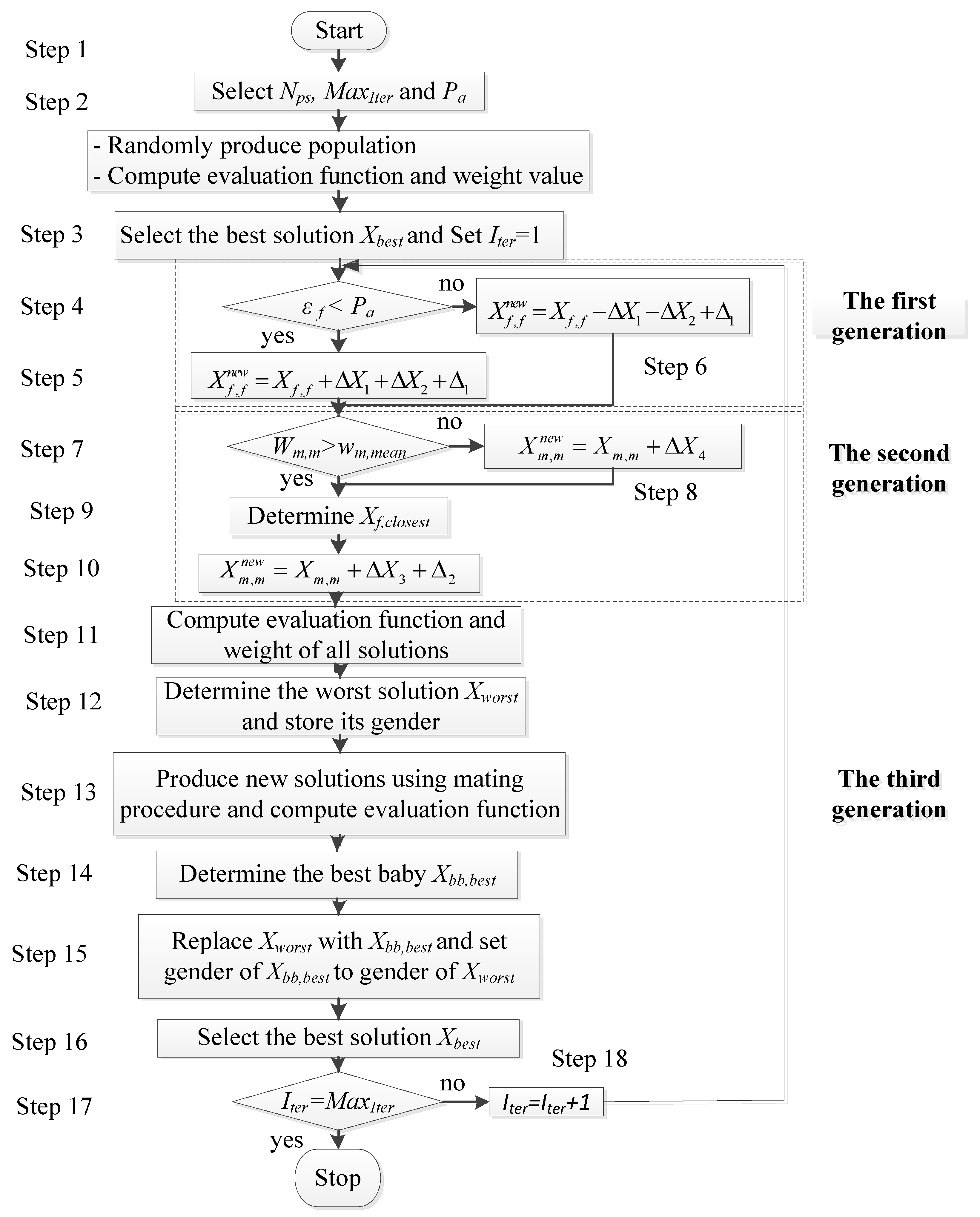
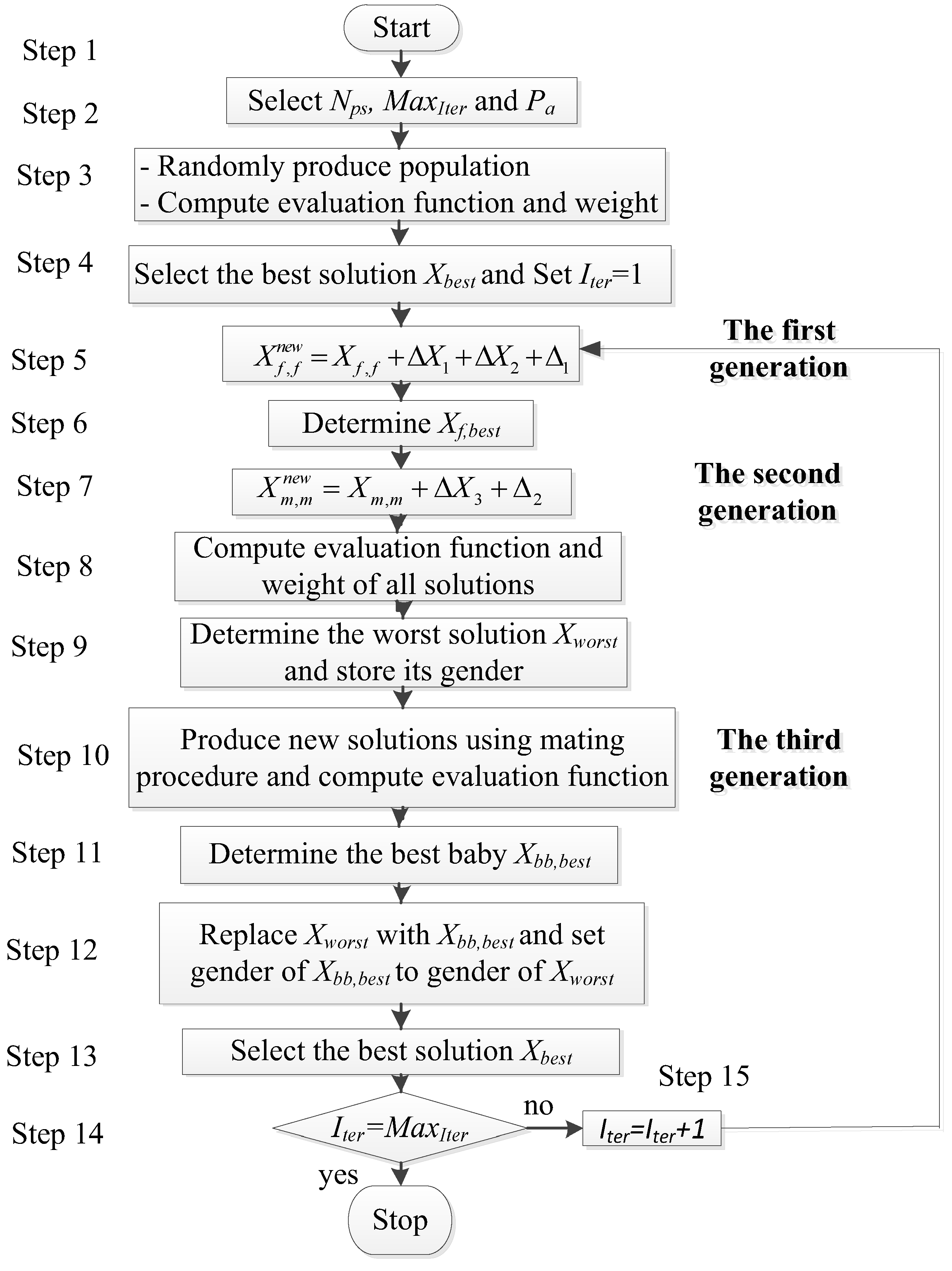
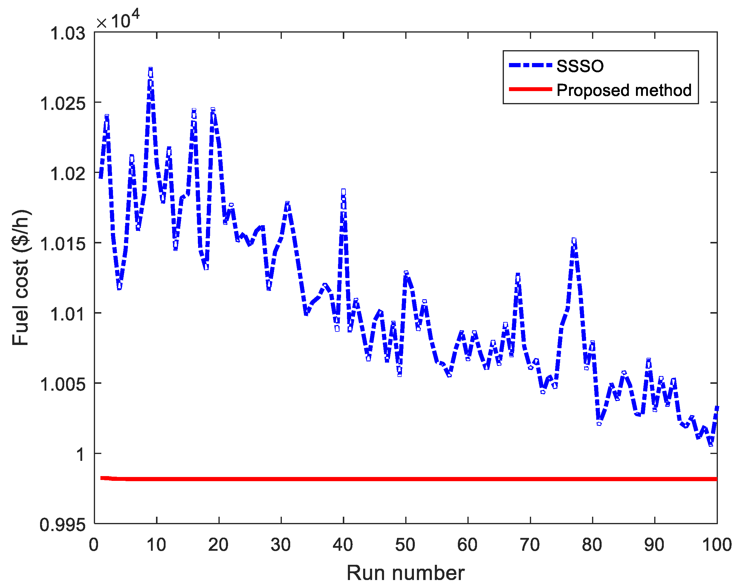
In general, authors have tended to apply original optimization tools or analyse these methods’ disadvantages and then they have proposed their improved methods in aim to find solution of ELD problem so that total electric generation fossil fuel cost could be lower than that from other existing methods. Similarly, in the paper we propose an effective social spider optimization algorithm, which is newly constructed from standard social spider optimization (SSSO) [46]. Similar to other methods, SSSO has been also tested on benchmark functions and its solutions have been competed to those of artificial bee colony (ABC) and PSO. Then, such method was newly developed and formed different modified SSO (MSSO) methods presented in [47,48,49]. MSSO in [47] has applied new strategy of predetermining the most effective solution. In the method, the best solution was continuously updated as soon as one new solution was produced and it was substituted into new candidate solution creation formula after it was identified. The proposed idea could move search space continuously and enrich exploration ability of SSSO but it also coped with other unintentionally weak points such as using higher number of computation steps and taking more simulation time than SSSO. MSSO in [48] has applied diversified mutation techniques similar to CCDE for seeking candidate solutions. Such modified method could intensify capability of seeking dominated solutions for SSSO but proposed ideas here also formed a MSSO method completely different from SSSO method. Unlike methods in [47,48], authors in [49] have developed four different modified SSSO (MSSO) methods by combining different modifications from PSO variants such as adding adaptive inertia weight and constriction factor, adding one more updated step size to new solutions. Their suggested ideas could enhance search ability of SSSO but it also caused more control parameters needing more selections and longer simulation time. Clearly, review on improved versions of SSSO can see that most methods have advantages as well as disadvantages, so in the paper we make a big effort introducing a new improved SSSO method so that the disadvantages of the mentioned MSSO methods above do not exist. In our ISSO method, we aim to reduce the computation steps, use of the most effective formulas, shortening simulation time and especially reduction of control parameter. For the target, we keep only one formula among two available equations of SSSO for the first and the second new solution creations. Then, we suggest changing such two retained equations so that they could create promising solutions. The proposed method’s superiorities can be investigated by testing on six systems with 6, 10, 15, 80, 160 and 320 units. In addition, different input-output characteristics and different constraints of thermal units and power systems are also considered. Results from the proposed method are compared to those from SSSO and other mentioned methods above. As a result, the main contributions of this paper are summarized as follows:

(1)

Simplify solution search procedure of SSSO.

(2)

Abandon less effective formulas producing low quality solutions and keep outstanding formulas.

(3)

Cancel some computation steps of SSSO.

(4)

Cancel one control parameter and quit tuning values of such parameter.

(5)

Find better solutions and use small number of iterations.

The organization of the remainder of the paper is as follows: in Section 2, we deal with the economic load dispatch problem formulation. Section 3 presents the main contents involving the development of the proposed method. The applications of the proposed method for the economic load dispatch problem have been stated in Section 4. Section 5 and the Appendix A present the study cases and numerical simulation results. Finally, the conclusions are given in Section 6.

2. Economic Load Dispatch (ELD) Problem Formulation

Such a considered ELD problem is clearly seen via the presence of objectives and a set of constraints of thermal generating units and power systems. In the paper, we consider six power systems wherein the major purpose aims to power output determination of available thermal generating units so that the power system performance is the best corresponding to the total minimized burnt fossil fuel cost. The major purpose and constraints are described in detail as follows.

2.1. The Major Purpose of ELD Problem

Each thermal generating unit n among the set of N units has consumed an amount of fossil fuel for its generated power. Corresponding to the fossil fuel amount, its cost FC_n in $/h is calculated and its efficiency is reflected via the cost. Thus, total fuel cost (TFC) of N units is considered as a major criterion for performance evaluation. Namely, the mathematical formula can be established as follows:

$$\mathrm{Minimize}\mathrm{TFC}={\displaystyle \sum _{n=1}^{N}F{C}_n}$$

(1)

where FC_n is burnt fossil fuel cost function with respect to power output of thermal generating unit n. FC_n corresponding to single fuel source and several fuel sources is, respectively, expressed by the following models:

$$F{C}_n={\mathsf{\alpha }}_n+{\mathsf{\beta }}_n{P}_n+{\mathsf{\chi }}_n{P}_n^2$$

(2)

$$F{C}_n=\{\begin{array}{l}{\mathsf{\alpha }}_{n1}+{\mathsf{\beta }}_{n1}{P}_n+{\mathsf{\chi }}_{n1}{P}_n^2\mathrm{for}{P}_n^{\min }\le P_n\le P_{n1}^{\max }\mathrm{and}\mathrm{fuel}1\\ {\mathsf{\alpha }}_{n2}+{\mathsf{\beta }}_{n2}{P}_n+{\mathsf{\chi }}_{n2}{P}_n^2\mathrm{for}{P}_{n2}^{\min }\le P_n\le P_{n2}^{\max }\mathrm{and}\mathrm{fuel}2\\ ⋮\\ {\mathsf{\alpha }}_{n{K}_n}+{\mathsf{\beta }}_{n{K}_n}{P}_n+{\mathsf{\chi }}_{n{K}_n}{P}_n^{2}for{P}_{n{K}_n}^{\min }\le P_n\le P_{n{K}_n}^{\max }\mathrm{and}\mathrm{fuel}{K}_n\end{array}$$

(3)

For the case considering fossil fuel sources and effects of working valves, Equation (3) becomes more complicated form as follows [20]:

$$F{C}_n=\{\begin{array}{l}{\mathsf{\alpha }}_{n1}+{\mathsf{\beta }}_{n1}{P}_n+{\mathsf{\chi }}_{n1}{P}_n^2+\left|{\mathsf{\delta }}_{n1}\times \sin ({\mathsf{\epsilon }}_{n1}\times (P_n^{\min }-P_n))\right|for{P}_n^{\min }\le P_n\le P_{n1}^{\max }\mathrm{and}\mathrm{fuel}1\\ {\mathsf{\alpha }}_{n2}+{\mathsf{\beta }}_{n2}{P}_n+{\mathsf{\chi }}_{n2}{P}_n^2+\left|{\mathsf{\delta }}_{n2}\times \sin ({\mathsf{\epsilon }}_{n2}\times (P_{n2}^{\min }-P_n))\right|for{P}_{n2}^{\min }\le P_n\le P_{n2}^{\max }\mathrm{and}\mathrm{fuel}2\\ ⋮\\ {\mathsf{\alpha }}_{n{K}_n}+{\mathsf{\beta }}_{n{K}_n}{P}_n+{\mathsf{\chi }}_{n{K}_n}{P}_n^2+\left|{\mathsf{\delta }}_{n{K}_n}\times \sin ({\mathsf{\epsilon }}_{n{K}_n}\times (P_{n{K}_n}^{\min }-P_n))\right|for{P}_{n{K}_n}^{\min }\le P_n\le P_{n{K}_n}^{\max }\mathrm{and}\mathrm{fuel}{K}_n\end{array}$$

(4)

2.2. Set of Constraints

In the section, constraints are arranged according to complex level where in the simplest constraint is mentioned first and the most complicated one is said at the end of the section. Firstly, generation capacity (GC) of each thermal generating unit is constrained. Secondly, the balance rule between generation source side and load demand side together with power loss is satisfied. For advanced power systems, other constraints such as generation increase and decrease range (GIDR), violated working zone (VWZ) and requested reserve real power (RRP) are taken into account. All the constraints are formulated as follows:

(i) Generation capacity constraint: Real power generation capacity of each thermal generating unit n is constrained by the following inequality:

$$P_n^{\min }\le P_n\le P_n^{\max };n=1,\mathrm{...},N$$

(5)

(ii) Demand side-supply side balance constraint: It needs to balance demand side (the sum of power of load and power loss in branches) and supply side (corresponding to total power generated by all thermal generating units) as the following rule:

$$P_{load}+P_{loss}={\displaystyle \sum _{n=1}^N{P}_n}$$

(6)

In Equation (6), P_loss is total power loss in all transmission lines and can be obtained by using power output of generating units and coefficients of active power loss matrix as follows:

$$P_{loss}={\displaystyle \sum _{n=1}^N{\displaystyle \sum _{j=1}^N{P}_n}}{B}_{nj}{P}_j+{\displaystyle \sum _{n=1}^N{B}_{0n}{P}_n+B_{00}}$$

(7)

where B_nj, B_0n and B₀₀ are coefficients of the power loss matrix. In order to calculate these B coefficients, the following steps should be applied [50].

(1)

Determine solution of power flow for initial operation state of power system: via the solution, magnitude and phase angles of voltage at all buses are known

(2)

Calculate load currents and total load current

(3)

Find Z impedance matrix

(4)

Determine transformation matrices C, ψ and H

(5)

Calculate B coefficients

However, it is noted that if new plans of generation and initial power system state are not highly different, the B coefficients may be considered to be constant [50]. For the ELD problem, these coefficients are known as given data and fixed at the same values during the process of determining the optimal power output of units [1]. These coefficients are not dependent on power output of generating units but total power loss P_loss is still influenced by the value of power output. This power loss calculation method is different from the method used in optimal power flow (OPF) problem. In OPF, P_loss is a more complicated function with the presence of voltage of buses, parameters of conductor and voltage phase angle of buses.

(iii) Violated working zone (VWZ) constraint: As mentioned in the constraint of Equation (5), power output of each unit must be within lower and upper bounds. However, due to the limitation of some components of unit, some zones inside the range are violated for operation. The zones are defined as violated working zone. As VWZ is considered, working power range of each thermal generating unit is not continuous as usual since several power intervals are violated for producing electricity. The typical VWZ is mathematically expressed by:

$$P_n\in \{\begin{array}{ll}{P}_{n,\mathrm{V}\mathrm{W}{\mathrm{Z}}_1}^{\min }\le P_n^{}\le P_{n,\mathrm{V}\mathrm{W}{\mathrm{Z}}_1}^{\max }& \\ ⋮& \\ P_{n,\mathrm{V}\mathrm{W}{\mathrm{Z}}_j}^{\min }\le P_n\le P_{n,\mathrm{V}\mathrm{W}{\mathrm{Z}}_j}^{\max }\\ ⋮& ;j=1,\mathrm{.....},\mathrm{N}\mathrm{V}\mathrm{W}{\mathrm{Z}}_n\\ P_{n,\mathrm{N}\mathrm{V}\mathrm{W}{\mathrm{Z}}_n}^{\max }\le P_n\le P_{n,\mathrm{N}\mathrm{V}\mathrm{W}{\mathrm{Z}}_n}^{\max }& \end{array}$$

(8)

where VWZ_j is the j-th violated working zone; NVWZ_n is the number of violated working zones of the n-th thermal generating unit;$P_{n,\mathrm{V}\mathrm{W}{\mathrm{Z}}_j}^{\min }$ and $P_{n,\mathrm{V}\mathrm{W}{\mathrm{Z}}_j}^{\max }$ are lower and upper bounds of the j-th violated working zone of the n-th thermal generating unit.

(iv) Required reserve power constraint: In order to avoid lack of energy in the case that the largest power unit shuts down, total active power reserve of all thermal units should be required to be equal to or higher than that of the largest power unit. The requirement is as below [20]:

$${\displaystyle \sum _{n=1}^N\left(P_n^{\max }-P_n^{}\right)}\ge P_{RR}^{}$$

(9)

where P_RR is the total requested reserve power of power system; $\left(P_n^{\max }-P_n^{}\right)$ is reserve power of the n-th thermal generating unit.

(v) Power generation increase and decrease limit constraint: The fact that thermal generating units cannot increase or decrease power generation immediately up to or down to expected power value but it needs time for the increase and decrease processes. Within one hour limit, power generation increase and decrease ranges are represented by PGI and PGD, and current generation must depend on such limits as two inequalities below:

$$P_n\ge P_n^{initial}-\mathrm{P}\mathrm{G}{\mathrm{D}}_n\mathrm{for}\mathrm{generation}\mathrm{decrease}\mathrm{purpose}$$

(10)

$$P_n\le P_n^{initial}+\mathrm{P}\mathrm{G}{\mathrm{I}}_n\mathrm{for}\mathrm{generation}\mathrm{increase}\mathrm{purpose}$$

(11)

where $P_n^{initial}$is the initial power of the n-th thermal generating unit; and PGI_n and PGD_n are allowed generation increase and decrease the step sizes of the n-th thermal generating unit.

3. The Proposed Improved Social Spider Optimization Algorithm (ISSO)

3.1. Review on Original Social Spider Optimization Algorithm

3.1.1. Spider Community

Spider community on the web is comprised of female spiders, male spiders and baby spiders wherein the population is supposed to be the sum of females and males while babies are not included in the population. The number of females is higher than that of males and it is approximately about from 60% to 90% of the whole population. Nature phenomenon of spider community is compatible with main steps in social spider optimization algorithm. Namely, SSSO and spider community can be described as follows:

(1)

Number of female spiders, NFS, is corresponding to NFS solutions

(2)

Number of male spiders, NMS, is corresponding to NMS solutions

(3)

Number of male and female spiders (NMFS) is population size (N_ps) and corresponding to a set of solutions

(4)

Movement of females is corresponding to newly updated procedure of NFS old solutions

(5)

Movement of males is corresponding to newly updated procedure of NMS old solutions

(6)

Mating males and females producing babies is corresponding to newly producing new solutions

As explained above, SSSO produces three generations of solution at each iteration. It newly produces NFS solutions for the first generation and NMS solutions for the second generation, but there is no an exact number of baby spiders or a number of solutions for the third generation.

3.1.2. The First Generation Producing NFS Solutions

The first generation is formed by two models of producing new solutions by using a condition, which compares a random number ε_f with a predetermined probability P_a. The two parameters are within the range from 0 to 1 but ε_f is randomly generated while P_a is manually selected. Each solution X_f,f owns one ε_f and it is newly updated based on comparison of ε_f and P_a. The mechanism is formulated as follows:

$$X_{f,f}^{new}=\{\begin{array}{ll}{X}_{f,f}^{}+\Delta X_1+\Delta X_2+{\Delta }_1& if{\epsilon }_f<P_a\\ X_{f,f}^{}-\Delta X_1-\Delta X_2+{\Delta }_1& else\end{array};f=1,\mathrm{...},NFS$$

(12)

where ∆X₁, ∆X₂ and ∆₁ are updated step sizes, which are calculated by:

$$\Delta X_1^{}={\phi }_1.V_{closest}.(X_{closest}-X_{f,f}^{})$$

(13)

$$\Delta X_2^{}={\phi }_2.V_{best}.(X_{best}-X_{f,f}^{})$$

(14)

$${\Delta }_1={\phi }_3.\left({\phi }_4-0.5\right)$$

(15)

The vibrations of the two spiders are calculated by the following expressions:

$$V_{closest}=W_{closest}.e^{-r_{{}_{closest}}^2}$$

(16)

$$V_{best}=W_{best}.e^{-r_{{}_{best}}^2}$$

(17)

In the two formulas above, r_closest and r_best are respectively the distance from the f-th female to one closest to her and to the best spider in the current population. W_closest and W_Gbest are weight values of the closest spider to the f-th female and the best spider. Weight value of each spider is calculated by using the following model:

$$W_s=\frac{E{F}_{worst}-E{F}_s}{E{F}_{worst}-E{F}_{best}}$$

(18)

where EF_worst and EF_best are evaluation function values of the worst and the best spiders; and EF_s is evaluation function value of the sth spider.

3.1.3. The Second Generation Producing NFS Solutions

Similar to the first generation, the second one also selects one out of two models for producing a new solution for each old considered solution. For diversity search purposes, SSSO classifies males into the good group with better weight than mean male and bad group with worse weight than mean male. Each one in the same group uses the same model but two ones in different groups use different models. The mechanism can be briefly described in the equation below:

$$X_{m,m}^{new}=\{\begin{array}{l}{X}_{m,m}^{}+\Delta X_3+{\Delta }_{2}if{W}_{m,m}>w_{m,mean}\\ X_{m,m}^{}+\Delta X_{4}else\end{array};m=1,\mathrm{....},NMS$$

(19)

In the formula, W_m,m and W_m,mean are weight value of the m-th male and mean weight value of all males, and other terms are calculated by the following models:

$$\Delta X_3^{}={\phi }_5.V_{f,closest}.(X_{f,closest}-X_{m,m}^{})$$

(20)

$${\Delta }_2={\phi }_6.({\phi }_7-0.5)$$

(21)

$$\Delta X_4^{}={\phi }_8.\left(\frac{{\displaystyle \sum _{m=1}^{NMS}{X}_{m,m}^{}.W_{m,m}}}{{\displaystyle \sum _{m=1}^{NMS}{W}_{m,m}}}-X_{m,m}^{}\right)$$

(22)

In Equation (20), X_f,closest and V_f,closest are the position and the vibration intensity of one female who is closest to the m-th male wherein such vibration is determined as follows:

$$V_{f,closest}=W_{f,closet}.e^{-r_{{}_{m,cloest}}^2}$$

(23)

where W_f,closest is weight value of one female who is closest to the m-th male; and r_m,closest is the length between such two spiders.

3.1.4. The Third Generation Producing NBS Solutions

The third generation may take place or not in each iteration depending on current status of all spiders in the web. At the beginning, average fitness of the whole population is determined and then males with less fitness function are considered to be dominated males. If dominant males can see any females within their supervised zone, they will mate with the females and producing babies. Otherwise, there is no mating issue happening in the web if females are not seen by dominant males. Such supervised zone of dominated males is a circle with radius R obtained by:

$$R=\frac{{\displaystyle \sum _{n=2}^N\left(\max (P_n^{})-\min (P_n^{})\right)}}{2\times (N-1)}$$

(24)

where max(P_n) and min(P_n) are the maximum and minimum values of P_n in all current solutions, X_m,m (m=1, …,NMS) and X_f,f (f=1, …, NFS).

After determining the radius of the circle, the dominant male and females in the circle will be mated, giving birth to babies as solutions. The b-th baby is formed as follows:

$$X_{bb,b}=[P_{2,b},P_{3,b},\mathrm{...},P_{n,b},\mathrm{..},P_{N,b}];b=1,\mathrm{..},NBS$$

(25)

where NBS is the number of baby spiders depending on the number of dominated males and the presence of females in his supervised zone; and P_n,b is power output of the n-th thermal generating unit of the b-th baby spider, which is randomly picked from dominated male and females in the circle. Among NBS baby spiders, only the best one X_bb,best is kept and the worst spider in population is replaced with X_bb,best. Then X_bb,best becomes male or female depending on the gender of the worst spider in the population. The whole search process of SSSO for a typical optimization problem can be performed as Figure 1.

3.2. The Proposed Algorithm

In the section, we carry out three modifications on the SSSO method where in the first and second modifications aim to change Equation (12) for the first generation and Equation (19) for the second generation but the third modification changes radius Equation (24).

3.2.1. The First Modification

In Equation (12), new solutions $X_{f,f}^{new}$ are updated by two models in which the first model adds three terms including ∆X₁, ∆X₂ and ∆₁ to old solutions X_f,f while the second model subtracts such three terms from such old solutions X_f,f. It is clear that the difference between the two models is adding or subtracting such three terms. As reviewing other meta-heuristic algorithms such as differential evolution with mutation operation [11,12], particle swarm optimization [16,17,18,19,20,21,22] and bat algorithm with velocity calculation Equation [37], cuckoo search algorithm with global search and local search [14,15], all the methods use addition of step sizes and there is no method using subtraction like the second model in Equation (11). Thus, the first modification is to use only the first model. As a result, Equation (11) is changed into the following model:

$$X_{f,f}^{new}=X_{f,f}^{}+\Delta X_1+\Delta X_2+{\Delta }_1;f=1,\mathrm{...},NFS$$

(26)

3.2.2. The Second Modification

In the second modification, we apply two changes. The first change is to use only the first model and cancel the second model in Equation (19). The second change is to replace the female closet to the considered male with the best female, who has been newly updated in Equation (26). As a result, the second generation in the proposed ISSO method is performed by the following model:

$$X_{m,m}^{new}=X_{m,m}^{}+\Delta X_3+{\Delta }_2 ;f=1,\mathrm{...},NMS$$

(27)

where:

$$\Delta X_3^{}={\phi }_5.V_{f,best}.(X_{f,best}-X_{m,m}^{})$$

(28)

$$V_{f,best}=W_{f,best}.e^{-r_{{}_{m,best}}^2}$$

(29)

where X_f,best and W_f,best are the position and weight of the best female; r_m,best is the length between the m-th male and the best female.

3.2.3. The Third Modification.

In the third modification, we change radius Equation (24) into the following model:

$$R=\frac{{\displaystyle \sum _{n=2}^N\left(P_n^{Max}-P_n^{Min}\right)}}{2\times (N-1)}$$

(30)

Observing that Equation (30) can prevent the radius while Equation (24) leads to different values for radius since iteration reaches the maximum value. In addition, the radius in Equation (24) tends to be decreased when iteration is high and it also narrows the search space of the third generation.

3.3. Optimization Problem

The whole search of the proposed ISSO method for solving a general optimization problem can be described as Figure 2.

4. The Application of the Proposed Method for ELD Problem

4.1. Randomly Producing Initial Population

As shown in Section 2, ELD problem absolutely consists of power output of thermal generating units and constraints. Thus, chosen decision variables are power output so that all constraints can be handled thoroughly and exactly. A set of (N−1) units is assigned to decision variables while another one is retained to be a balance variable. Such selection method can prevent constrain (6) from violating and punish the balance variable only. Thus, initial population can be randomly generated within the range as the following rule:

$$X_{}^{\min }\le X_s\le X_{}^{\max };s=1,\mathrm{.....},N_{ps}$$

(31)

where X_s is position of the s-th spider and corresponding to solution s; X^min and X^max are the minimum and maximum generation of (N−1) decision variables. The terms are mathematically expressed by:

$$X_s=[P_{2,s},P_{3,s},\mathrm{...},P_{n,s},\mathrm{..},P_{N,s}];s=1,\mathrm{..},NMFS$$

(32)

$$X^{\min }=[P_2^{\min },P_3^{\min },\mathrm{...},P_n^{\min },\mathrm{..},P_N^{\min }]$$

(33)

$$X^{\max }=[P_2^{\max },P_3^{\max },\mathrm{..},P_N^{\max }]$$

(34)

4.2. Solution Evaluation Function Construction

Evaluation function is used to rank the quality of solutions. Normally, the evaluation function considers the objective and punishment of constraints. Objective can be easily computed as using (1)–(4) while punishment of constraints should be meticulously considered because wrong punishment leads to invalid solutions violating constraints. In the paper, there are five constraints of ELD problem taken into account such as generation capacity, demand side-supply side balance, generation increase and decrease range, violated working zone and requested reserve real power. The punishment of the constraints are handled as follows:

(i) Generation capacity violation punishment

There is no punishment for the constraint because all decision variables are verified and corrected if they are outside the allowed range. Namely, decision variables are set to minimum value if they are lower than the minimum and they are set to maximum value if they are higher than the maximum.

(ii) Demand side-supply side balance violation punishment

The violation of the constraint is converted to the violation of thermal unit 1 because thermal unit 1 is obtained as follows:

$$P_1=P_{load}+P_{loss}-{\displaystyle \sum _{n=2}^N{P}_n}$$

(35)

By substituting Equation (7) into Equation (35), a second order equation with respect to P₁ is determined as follows:

$$B_{11}{P}_1^2+\left(2{\displaystyle \sum _{n=2}^N{B}_{1n}{P}_n}+B_{01}-1\right)P_1+\left(P_D+{\displaystyle \sum _{n=2}^N{\displaystyle \sum _{j=2}^N{P}_n{B}_{nj}{P}_j}+{\displaystyle \sum _{n=2}^N{B}_{0n}{P}_n}}+B_{00}-{\displaystyle \sum _{n=2}^N{P}_n}\right)=0$$

(36)

By solving the second order equation, P₁ is calculated by:

$$P_1=\frac{-\left(2{\displaystyle \sum _{n=2}^N{B}_{1n}{P}_n}+B_{01}-1\right)\pm \sqrt{\Delta }}{2B_{11}}$$

(37)

where:

$$\Delta ={\left(2{\displaystyle \sum _{n=2}^N{B}_{1n}{P}_n}+B_{01}-1\right)}^2-4B_{11}\left(P_D+{\displaystyle \sum _{n=2}^N{\displaystyle \sum _{j=2}^N{P}_n{B}_{nj}{P}_j}+{\displaystyle \sum _{n=2}^N{B}_{0n}{P}_n}}+B_{00}-{\displaystyle \sum _{n=2}^N{P}_n}\right)$$

(38)

Here, P₁ is already known but the guarantee that P₁ is always within its allowed range is not made. In fact, P₁ can violate lower bound or upper bound. Thus, it should be checked and penalized by using the following model:

$$Pus{h}_{P_1}=\{\begin{array}{ll}0& if{P}_1\in [P_1^{\min },P_1^{\max }]\\ \left|P_1-P_1^{\min }\right|& if{P}_1\in (-\infty ,P_1^{\min })\\ \left|P_1-P_1^{\max }\right|& if{P}_1\in (P_1^{\max },+\infty )\end{array}$$

(39)

In summary, the violation of power balance constraint is dependent on the violation of P₁ meanwhile the violation of P₁ can be checked and penalized thank to the use of Equation (39). The penalty of P₁ is included in fitness function and then the proposed ISSO will find optimal solutions without any violations.

(iii) Generation increase and decrease range violation punishment

As the n-th unit violates the constraint, it is also punished by lower interval of accepted minimum value ($P_n^{initial}-\mathrm{P}\mathrm{G}{\mathrm{D}}_n$) or higher interval of accepted maximum value ($P_n^{initial}+\mathrm{P}\mathrm{G}{\mathrm{I}}_n$). The punishment is described by the following model:

$$Pus{h}_{GID{R}_n}=\{\begin{array}{l}0if{P}_n^{initial}-\mathrm{P}\mathrm{G}{\mathrm{D}}_n\le P_n\le P_n^{initial}+\mathrm{P}\mathrm{G}{\mathrm{I}}_n\\ \left|P_n-P_n^{initial}-\mathrm{P}\mathrm{G}{\mathrm{I}}_n\right|if{P}_n>P_n^{initial}+\mathrm{P}\mathrm{G}{\mathrm{I}}_n;n=1,\mathrm{....},N\\ \left|P_n^{initial}-\mathrm{P}\mathrm{G}{\mathrm{D}}_n-P_n\right|if{P}_n<P_n^{initial}-\mathrm{P}\mathrm{G}{\mathrm{D}}_n\end{array}$$

(40)

(iv) Violated working zone violation punishment

As the power output of unit n has fallen into one of violated working zones, it is punished. The bound of punishment is mean of minimum and maximum generation of the VWZ. The detail is as follows:

$$Pus{h}_{\mathrm{V}\mathrm{W}\mathrm{Z}}{}_n\in \{\begin{array}{l}0if{P}_n\notin [P_{n,\mathrm{V}\mathrm{W}{\mathrm{Z}}_j}^{\min },P_{n,\mathrm{V}\mathrm{W}{\mathrm{Z}}_j}^{\max }]\\ \left|P_n-P_{n,\mathrm{V}\mathrm{W}{\mathrm{Z}}_j}^{\min }\right|if{P}_n\in [P_{n,\mathrm{V}\mathrm{W}{\mathrm{Z}}_j}^{\min },P_{n,\mathrm{V}\mathrm{W}{\mathrm{Z}}_j}^{\max }]\&\left(P_n<P_{n,\mathrm{V}\mathrm{W}{\mathrm{Z}}_j}^{mean}\right)\\ \left|P_n-P_{n,\mathrm{V}\mathrm{W}{\mathrm{Z}}_j}^{\max }\right|if{P}_n\in [P_{n,\mathrm{V}\mathrm{W}{\mathrm{Z}}_j}^{\min },P_{n,\mathrm{V}\mathrm{W}{\mathrm{Z}}_j}^{\max }]\&\left(P_n>P_{n,\mathrm{V}\mathrm{W}{\mathrm{Z}}_j}^{mean}\right)\end{array}$$

(41)

where:

$$P_{n,\mathrm{V}\mathrm{W}{\mathrm{Z}}_j}^{mean}=\frac{P_{n,\mathrm{V}\mathrm{W}{\mathrm{Z}}_j}^{\min }+P_{n,\mathrm{V}\mathrm{W}{\mathrm{Z}}_j}^{\max }}{2};j=1,\dots ,\mathrm{N}\mathrm{V}\mathrm{W}\mathrm{Z}\&n=1,\dots ,N$$

(42)

(v) Requested reserve power violation punishment

Since the total reserve power of all units is less than requested reserve power of power system, solution is punished. Otherwise, the solution is not punished if the total reserve power is equal to or higher than RRP. Namely, the following formula can give the exact punishment for RRP violations:

$$Pus{h}_{RRP}=\{\begin{array}{ll}0& if{\displaystyle \sum _{n=1}^N\left(P_n^{\max }-P_n^{}\right)}\ge P_{RR}\\ \left|{\displaystyle \sum _{n=1}^N\left(P_n^{\max }-P_n^{}\right)}-P_{RR}^{}\right|& else\end{array}$$

(43)

As a result, the evaluation function is formed as follows:

$$EF=\left({\displaystyle \sum _{n=1}^{N}F{C}_n}\right)+K_{push}{\left(Pus{h}_{P_1}\right)}^2+K_{push}{\left({\displaystyle \sum _{n=1}^N(Pus{h}_{GID{R}_n}}+Pus{h}_{VWZ}{}_n)\right)}^2+K_{push}{\left(Pus{h}_{RRP}\right)}^2$$

(44)

4.3. Termination Criterion

Generally, the stopping criterion for methods solving optimization problems are usually based on the iterative errors of two consecutive iterations, constraint mismatch, and maximum number of iterations depending on applied methods. In the paper, the proposed ISSO is a metaheuristic method which is influenced by randomization. Thus, the termination criterion should be based on the maximum number of iterations, Max_Iter. The whole search procedure for one optimal solution is not terminated until the current iteration is equal to Max_Iter. The selection of Max_Iter is done by referring to other studies for the same problem and using trial and error method. However, for approximately all cases, quality of found solutions is dependent on both Max_Iter and population size N_ps in which N_ps directly influences the best optimal solution of the current iteration and execution time of one iteration while Max_Iter directly influences the final optimal solution of one run and execution time of one run. The proposed ISSO method handles constraints (6), (8)–(11) by using control variables shown in (25) and other penalty methods in equations (39)–(43) so that all constraints are always satisfied. One solution is considered to be optimal if it can satisfy all constraints shown in problem formulation section and its objective function is not very high. Normally, one solution, which is found by using optimization algorithm, is called optimal solution but it is not sure that its quality is the best. In our study, we have known the optimal solutions of previous studies as well as values of control parameters. Thus, we have tried from small values to high values for N_ps and Max_Iter until the optimal solution have been equal or better than those of previous studies. However, due to the outstanding performance of the proposed ISSO, normally the most appropriate values are less than those from previous studies.

5. Numerical Results

In order to judge the improvement level of the proposed method over SSSO as well as search ability compared to other existing methods in solving ELD problem, it together with SSSO are applied in the work of finding solutions of six systems including 6, 10, 15, 80, 160 and 320 thermal generating units. Diversification of systems is in turn taken into account when considering different data such as single fuel source, multiple fuel sources, multiple fuel sources with valve effects as well as different constraints such as generation capacity (GC), demand side-supply side balance (DSB), generation increase and decrease range (GIDR), violated working zone (VWZ) and requested reserve power (RRP). For the sake of easy observation, six systems with seven cases are described in detail in

Table 1. The selection of population size and the highest iteration number.

System	No. Units	Characteristic	Constraints	Nps	MaxIter
1	6	Single fuel source	GC, DSB, VWZ	20	30
2	10	Multiple fuel sources and valve effects	GC, DSB	30	40
	10	Multiple fuel sources and valve effects	GC, DSB, VWZ, GIDR, RRP	40	50
3	15	Single fuel source	GC, DSB, VWZ, RRP	10	100
4	80	Multiple fuel sources and valve effects	GC, DSB	20	400
5	160	Multiple fuel sources and valve effects	GC, DSB	30	500
6	320	Multiple fuel sources and valve effects	GC, DSB	30	1000

. The proposed method and SSSO are developed in programming language of Matlab 9.0 and run on laptop with 2.4 Ghz processor and 4GB RAM. For comparisons, 100 trial runs are independently obtained for each case.

5.1. Testing Contribution of the Proposed Modifications

In this section, we have investigated the contribution of each proposed modification on the results obtained by ISSO, so in addition to SSSO and ISSO, we have also implemented three other versions of SSSO consisting of SSSO with the first modification (called ISSO1), SSSO with the second modification (called ISSO2) and SSSO with the third modification (called ISSO3) for three systems 1, 3 and 6. The three selected systems have different characteristics such as different constraints, different numbers of units and different fuel cost functions. The results summarized in

Table 2. Results obtained by ISSO and other versions of SSSO for three systems 1, 3 and 6.

System	Method	Minimum Cost ($)	Mean Cost ($)	Maximum Cost ($)	Success Rate (%)
1	SSSO	15,443.076	15,443.09	15,443.32	76%
	ISSO1	15,443.0749	15,443.081	15,443.26	100%
	ISSO2	15,443.0749	15,443.082	15,443.18	100%
	ISSO3	15,443.0749	15,443.088	15,443.28	100%
	ISSO	15,443.0749	15,443.077	15,443.12	100%
3	SSSO	32,599.07	32,645.30	32,711.26	69%
	ISSO1	32,545.03	32,548.88	32,568.05	100%
	ISSO2	32,545.72	32,549.23	32,563.62	100%
	ISSO3	32,565.00	32,578.71	32,609.24	88%
	ISSO	32,544.97	32,545.45	32,561.79	100%
6	SSSO	20,294.16	20,962.64	21,482.06	100%
	ISSO1	19,965.35	19,968.18	19,997.03	100%
	ISSO2	19,964.87	19,970.74	19,994.86	100%
	ISSO3	19,987.02	19,995.66	20,024.71	100%
	ISSO	19,963.14	19,964.46	19,989.38	100%

are minimum cost, mean cost, maximum cost and success rate. The success rate is a ratio of the number of successful runs (100 runs) to the total number of runs where the total number of runs is the sum of the number of successful runs and the number of unsuccessful runs. Here, a run is called a successful run if the final optimal solution of the run can satisfy all constraints or the fitness function of the optimal solution is equal to its total fuel cost. By observing the success rate values, the effectiveness of each modification can be identified clearly. Both ISSO1 and ISSO2 together with ISSO could deal with all constraints absolutely since they have reached a success rate of 100% for the three systems. ISSO3 could not be as good as ISSO1, ISSO2 and ISSO but it was better than SSSO since its success rates were, respectively, 100%, 88% and 100% for the three systems while those of SSSO were, respectively, 76%, 69% and 100% for systems 1, 3 and 6. It can be easily understood that system 3 is the most complicated with four types of constraint and system 6 is the simplest with only two types of constraint. The minimum cost of each system obtained by the five methods can lead to a conclusion that SSSO has found the worst optimal solutions with the highest cost for all systems. For the system 1, ISSO1, ISSO2, ISSO3 and ISSO have reached the same fuel cost, which was less than that of SSSO. For the systems 3 and 6, ISSO1, ISSO2 and ISSO3 have found lower minimum cost than SSSO but higher minimum cost than ISSO. The comments on mean cost and maximum cost obtained by these methods are also similar to those on the minimum cost. Consequently, it can be stated that each proposed modification could improve result better than SSSO for three systems in terms of dealing with constraints and finding optimal solutions with high quality.

5.2. Result Comparisons on the First System

In this section, the challenge for the proposed method’s robustness and effectiveness is to find solutions of a six-unit system taking VWZ constraint and power loss in branches into account. Load-side power is 1263 MW. For the data of the system, readers can refer to [51]. One hundred values of the fuel cost are obtained for both SSSO and the proposed methods by setting the population size and maximum iterations to 20 and 30, respectively.

Table 3. Result summary obtained by different methods and the proposed method for system 1 with 6 units.

Method	Minimum Cost ($)	Mean Cost ($)	Maximum Cost ($)	IP (%)	CPU Time (s)	Nps	MaxIter	Nnspr
DE [11]	15449.7660	15449.7770	15449.8740	0.043	33.5	36	100	3600
GA [11]	15459.0000	15469.0000	15524.0000	0.103	NR	NR	NR	-
PSO [11]	15450.0000	15454.0000	15492.0000	0.045	NR	NR	NR	-
PSO [16]	15450.0000	15454.0000	15492.0000	0.045	NR	20	50	1000
LRS-MPSO [16]	15450.0000	15450.5000	15452.0000	0.045	NR	20	50	1000
GA [16]	15459.0000	15469.0000	15524.0000	0.103	NR	20	50	1000
LRS-PSO [16]	15450.0000	15454.0000	15455.0000	0.045	NR	20	50	1000
MPSO [16]	15450.0000	15452.0000	15454.0000	0.045	NR	20	50	1000
SUP-PSO [17]	15446.0200	15497.3500	15609.6400	0.019	0.0633	30	125	3750
PSO [18]	15450.0000	15454.0000	15492.0000	0.045	11.3	90	100	9000
FPSO [18]	15445.2440	15448.0520	15451.6300	0.014	8.7	60	100	6000
NAPSO [18]	15443.7656	15443.7657	15443.7657	0.004	3.2	30	100	3000
IPSO [20]	15444.0000	15446.3000	NR	0.006	NR	20	200	4000
IPSO-TVAC [21]	15443.0630	15443.5820	155445.1140	0.000	NR	40	60	2400
KHA-I [23]	15450.7492	15452.8220	15455.5000	0.050	NR	50	100	10,000
KHA-II [23]	15448.2117	15450.8320	15453.4000	0.033	NR	50	100	10,000
KHA-III [23]	15445.3560	15447.2180	15449.6000	0.015	NR	50	100	10,000
KHA-IV [23]	15443.0752	15443.1860	15443.3000	0.000	NR	50	100	10,000
OKHA [24]	15443.0750	15443.9160	15443.3270	0.000	NR	NR	100	-
IFA [31]	15443.075	15443.1270	15443.5389	0.000	NR	10	30	1650
BFA [33]	15443.8497	15 446.95383	NR	0.005	NR	NR	30,000	-
MTS [34]	15450.0600	15451.1700	15453.64	0.045	1.29	10	200	2000
EMA [39]	15443.0749	15443.0750	NR	0.000	0.0024	NR	NR	-
SSSO	15443.076	15443.09	15443.32	0.000	0.2	20	30	≈690
ISSO	15443.0749	15443.077	15443.12	0.000	0.14	20	30	≈690

NR: Not reported.

reports the best solution’s fuel cost, the worst solution’s fuel cost and average fuel cost of all solutions together with control parameters from SSSO, the proposed method and other existing methods. It is indicated by the table that the proposed method can minimize the generation cost more effectively than SSSO since the best solution, the worst solution and average solution of the proposed method have less generation cost than those of SSSO. Furthermore, it is clearly visible by observing Figure 3 that approximately 94 solutions of the proposed methods have better generation costs than those from SSSO. Thus, sufficient evidences such as better best solution, better worst solution and approximately all better solutions can justify the improvement level of the proposed method over SSSO for the system. Comparing the proposed method with other reported methods also sees that the proposed method is superior to DE [11], GA [11], PSO [11], GA [16], PSO [16], LRS-MPSO [16], GA [16], LRS-PSO [16], SUP-PSO [17], PSO [18], FPSO[18], NAPSO [18] , IPSO [20], IPSO-TVAC [21], KHA-I [23], KHA-II [23], KHA-III [23], BFA [33] and MTS [34] with respect to the best solution while the average solution and the worst solution from the proposed method are approximate to or better than those from others. As seen in the fifth column, the improvement percentage (IP) values of the best solution from the proposed method over other ones is not high, just from 0% to 0.103% but the population size and iterations employed for the proposed method are smaller than those from all methods with reported values. N_ps and Max_Iter were set to 20 and 30 for the proposed method but they were 20 and 50 for the methods in [16], 30 and 125 for the method in [17], 30 and 100 for the methods in [18], 40 and 60 for the methods in [21], and 10 and 200 for the method in [34]. Thus, the proposed method has used about 690 newly updated solutions and spent 0.14 seconds, while that from other methods was from 1000 to 10,000 solutions. It is clear that if these methods have been run by setting N_ps and Max_Iter to the same values as the proposed method, their results, i.e. minimum, average and maximum cost, would be increased to higher values and their performance would be much worse than the proposed method because their iterations would be decreased from 2 to 7 times as compared to reported values. As a result, we can state that the proposed method is capable of finding better results than most methods for the system with VWZ and transmission power loss. The best solution found by the proposed method is given in

Table A1. The best decision variables for systems 1 found by the proposed method.

Unit n	Pn (MW)
2	173.2409
3	263.3816
4	138.9797
5	165.3918
6	87.0516

in the Appendix A.

5.3. Result Comparisons on the Second System

In this study case, the proposed method together with SSSO are applied to the second system with ten units using multiple fossil fuel sources in which the first case considers valve effects and load-side and supply side balance constraint while the second case considers such constraints together with other constraints such as VWZ, GIDRC and RRPC. The whole data of the first case and the second case are taken from [27] and [28], respectively. Results of different methods are reported in

Table 4. Result summary obtained by different methods and the proposed method for case 1 of system 2.

Method	Minimum Cost ($)	Mean Cost ($)	Maximum Cost ($)	IP (%)	CPU Time (s)	Nps	MaxIter	Nnspr
ORCSA [15]	623.8684	623.9495	626.3666	0.006	1.58	12	500	12,000
CCDE [12]	623.8288	623.8574	623.8904	0.000	NR	35	200	7000
CSA [14]	623.8684	623.9495	626.3666	0.006	0.679	10	500	10,000
KHA-I [23]	611.3276	613.0895	614.8293	−2.045	NR	20	500	20,000
KHA-II [23]	609.0768	610.3271	611.2105	−2.422	NR	20	500	20,000
KHA-III [23]	607.5437	608.1164.	608.5431	−2.680	NR	20	500	20,000
KHA-IV [23]	605.7582	605.8043	605.9426	−2.983	NR	20	500	20,000
FA [31]	664.5306	675.5344	679.426	6.125	NR	10	100	5500
IFA [31]	623.8768	625.2704	629.2765	0.008	NR	10	100	5500
UM-GA [27]	624.7193	627.6087	633.8652	0.143	26.17	30	30	1800
UM-MGA [27]	624.5178	625.8692	630.8705	0.110	7.25	30	30	1800
MRCGA [28]	623.8307	623.8522	623.8908	0.000	5.45	10	300	6000
SSSO	623.9631	624.2205	627.6094	0.022	0.6	30	100	≈4200
ISSO	623.8286	623.8490	624.1641	-	0.23	30	40	≈1500

and

Table 5. Result summary obtained by different methods and the proposed method for case 2 of system 2.

Method	Minimum Cost ($)	Mean Cost ($)	Maximum Cost ($)	IP (%)	CPU Time (s)	Nps	MaxIter	Nnspr
RCGA [28]	624.6605	625.9201	628.9253	0.050	34.61	10	300	6000
MRCGA [28]	624.3550	624.5792	624.7541	0.001	7.43	10	300	6000
FA [31]	673.5544	685.2872	699.2855	7.306	NR	10	300	6000
IFA [31]	624.4951	625.2647	629.3951	0.024	NR	10	300	3000
SSSO	624.5460	625.2707	629.1719	0.032	0.5	40	50	≈2460
ISSO	624.3477	624.3666	624.8145	-	0.38	40	50	≈2445

for case 1 and case 2, respectively. Comparison between SSSO and the proposed method can justify the outstanding search of the proposed method since it can find better set of solutions reflected via better minimum cost, average cost and maximum cost than those from SSSO. The best minimum also indicates that the proposed method can reach the same search ability as some methods or can improve solution search ability up to 6.125%. Moreover, the proposed method is run by setting 40 iterations but SSSO is implemented by using 100 iterations. Once more, the better search ability of the proposed method over SSSO can be seen via 100 generation cost values over 100 runs shown in Figure 4 and Figure 5. For other comparisons with the remaining methods seen in Table 4, KHA methods can find better solutions and reach better robustness than the proposed method; however, real fuel types and reported fuel types do not fit together, and recalculated fuel cost is much higher than that of the proposed method. On the other hand, the proposed method can find better solutions with lower minimum cost, lower average cost and lower maximum cost than all methods excluding CCDE [12] and MRCGA [28] for maximum cost comparison. The best minimum also indicates that the proposed method can improve solution search ability from 0.001% to 7.306%. Moreover, the proposed method is the fastest one in finding the best optimal solution since it has used only about 1500 solutions while compared methods have used from 1800 to 20,000 solutions. Consequently, it is pointed out that the proposed method is one of the most powerful methods for the first case of the system. Similarly, results reported in Table 5 also give the same evaluation since the proposed method can find the least minimum cost, the least average cost and the second least maximum cost among presented methods. For convergence speed comparison, the proposed method is also the strongest one since it has used approximately 2445 newly updated solutions meanwhile that of others has been from 3000 to 6000. The best solution found by the proposed method is given in

Table A2. The best decision variables for system 2 found by the proposed method.

Case 1		Case 2
Unit n	Pn (MW)	Unit n	Pn (MW)
2	212.6498	2	211.226
3	280.6571	3	282.7304
4	239.4176	4	241.5215
5	279.8815	5	260
6	239.2578	6	239.9184
7	287.7275	7	292.5613
8	239.9551	8	242.6034
9	426.4820	9	438.6131
10	275.8665	10	270

in the Appendix A.

5.4. Results Comparisons on the Third System

In this part, the third system with 15 units considering complicated VWZ and RRP constraints and simple power balance constraint is used for judging the best solution as well as the search stability of the proposed method. The whole data of the system can be seen in [52]. Generation cost of the most effective runs, the least effective run and all runs on average are summarized in

Table 6. Result summary obtained by different methods and the proposed method for system 3.

Method	Minimum Cost ($)	Mean Cost ($)	Maximum Cost ($)	IP (%)	CPU Time (s)	Nps	MaxIter	Nnspr
CSA [14]	32,544.97	32,545.01	32,546.67	0.00	0.589	10	400	8000
ORCSA [15]	32,542.56	32,543.17	32,546.66	−0.01	0.468	12	500	9600
FA [31]	32,885.84	-	-	1.04	NR	10	100	5500
IFA [31]	32,544.97	32,545.22	32,545.54	0.00	NR	10	100	5500
KHA-I [23]	32,586.75	32,592.04	32,598.02	0.13	NR	50	100	10,000
KHA-II [23]	32,569.80	32,571.45	32,573.63	0.08	NR	50	100	10,000
KHA-III [23]	32,564.39	32,566.58	32,567.33	0.06	NR	50	100	10,000
KHA-IV [23]	32,547.37	32,548.14	32,548.93	0.01	NR	50	100	10,000
SSSO	32,599.07	32,645.30	32,711.26	0.17	2.4	50	500	≈3015
ISSO	32,544.97	32,545.45	32,561.79	-	0.18	10	100	≈1243

. Such results confirm the superiority of the proposed method over SSSO in addition to a smaller population size and less iterations. Comparing with other methods also leads to approximately the same conclusion since the proposed method finds similar best solutions as CSA [14] and IFA [31], and finds a better best solution than other methods except for ORCSA [15]. For exact comparison, IP values indicate that the proposed method can get the same performance as some methods and can improve the performance to 1.04% as compared to the worst method. However, control parameter comparison can report the fastest search ability of the proposed method because it has used about 1,200 new solutions while others have used from 5,500 to 10,000 new solutions. Figure 6 sees a high deviation between the proposed method and SSSO when all solutions of the proposed method are approximately on a line and much less than those from SSSO. The best solution found by the proposed method is given in

Table A3. The best decision variables for system 3 found by the proposed method.

Unit n	Pn (MW)	Unit n	Pn (MW)	Unit n	Pn (MW)
2	436.1776	6	447.5354	11	20.0000
3	130.0000	7	465.0000	12	53.5292
4	130.0000	8	60.0000	13	25.0000
5	308.1706	9	25.0000	14	15.0000
		10	20.0000	15	15.0000

in the Appendix A.

5.5. Results Comparisons on the Fourth System

In the fourth system, 80 units with valve effects and multiple fuels are considered to supply electricity to a load of 21,600 MW. The whole data of the system can be seen in [27]. The minimum generation cost from the best power output, the maximum generation cost from the worst power output together with average generation cost of 100 runs obtained by the proposed method and other ones are shown in

Table 7. Result summary obtained by different methods and the proposed method for system 4.

Method	Minimum Cost ($)	Mean Cost ($)	Maximum Cost ($)	IP (%)	CPU Time (s)	Nps	MaxIter	Nnspr
CSA [14]	4992.685	4993.731	5003.429	0.036	18.257	10	2000	40,000
ORCSA [15]	4992.422	4994.499	4995.672	0.031	15.24	12	5500	132,000
UM-GA [27]	-	5008.143	-	-	309.41	30	90,000	5,400,000
UM-MGA [27]	-	5003.883	-	-	85.67	5	90,000	900,000
SSO	4993.455	5002.910	5097.825	0.052	4.2	70	400	≈33,100
ISSO	4990.868	4991.198	4993.871	-	1.1	20	400	≈10,261

. All costs show that the proposed method can find a better set of solutions than all methods for the case because all the cost values from the proposed method are less than those from other compared ones. The values of IP indicate that the proposed method can improve the best solution quality from 0.031% to 0.052% over other methods. Moreover, the proposed method is also faster than all methods for converging to the best solution since it uses under 11,000 new solutions but others use from about 33,000 to 5,400,000 new solutions. Figure 7 reports a huge difference of effectiveness between the proposed method and SSSO. The best solution found by the proposed method is reported in

Table A4. The best decision variables for system 4 found by the proposed method.

Unit n	Pn (MW)	Unit n	Pn (MW)	Unit n	Pn (MW)	Unit n	Pn (MW)
2	211.9071	21	217.078	41	217.078	61	217.078
3	279.6489	22	211.9071	42	211.9071	62	211.9071
4	241.4332	23	279.6489	43	279.6489	63	282.6735
5	279.872	24	238.0739	44	241.4332	64	241.4332
6	239.3922	25	276.3352	45	279.872	65	279.872
7	287.7271	26	239.3922	46	239.2578	66	239.3922
8	239.4176	27	287.7271	47	287.7275	67	287.7271
9	430.6942	28	239.4176	48	239.4176	68	239.6864
10	272.6941	29	431.3281	49	430.6942	69	430.6942
11	217.078	30	272.6941	50	275.8546	70	272.6941
12	211.9071	31	217.078	51	217.078	71	217.078
13	279.6489	32	211.9071	52	211.9071	72	211.9071
14	241.4332	33	279.6489	53	279.6489	73	279.6489
15	279.8721	34	241.4332	54	241.4332	74	241.4332
16	239.3922	35	279.8718	55	279.8717	75	279.8718
17	287.7272	36	239.3922	56	239.3922	76	239.3922
18	239.4176	37	287.727	57	287.7271	77	287.7271
19	430.6942	38	239.4176	58	239.4176	78	239.4175
20	272.6941	39	430.6942	59	430.6942	79	430.6943

in the Appendix A.

5.6. Results Comparisons on the Fifth System

In this section, the fifth system with three fuel sources for each thermal generating unit and considering valve point effects on thermal generating units is employed to run the proposed method and SSSO. Load-side power is 43,200 MW. For the entire data of the system readers can refer to [27]. Result comparisons between the proposed method with SSSO and other ones are given in

Table 8. Result summary obtained by different methods and the proposed method for system 5.

Method	Minimum Cost ($)	Mean Cost ($)	Maximum Cost ($)	IP (%)	CPU Time (s)	Nps	MaxIter	Nnspr
CSA [14]	9990.66	9996.64	10,014.02	0.090	75.429	10	6000	120,000
ORCSA [15]	9989.94	9992.05	9996.83	0.083	67.50	12	8000	192,000
TLA [26]	10,005.99	10,006.01	10,006.28	0.243	48.216	50	1000	50,000
UM-GA [27]	-	10,143.73	-		621.30	30	90,000	5,400,000
UM-MGA [27]	-	10,042.47	-		174.62	5	90,000	900,000
CBA [37]	10,002.86	10,006.33	10,045.23	0.212	5.71	40	500	40,000
SOS [44]	10,121.21	10,179.03	10,241.08	1.379	NR	20	60	72,000
ISOS [44]	9981.31	9981.98	9,983.64	−0.003	25.72	20	60	72,000
ORCCRO [45]	10,004.20	10004.21	10,004.45	0.225	0.019	48	1000	48,000
SSSO	10,005.13	10,105.81	10,274.97	0.235	5.8	70	800	≈62,215
ISSO	9981.65	10,007.94	10,026.58	-	1.6	30	500	≈18,478

. For implementing SSSO and the proposed method, we have tried to set the population and iterations to 30 and 500 but the results from SSSO were too bad. Thus, we have continued to test its performance by increasing the values to 70 for population and 800 for iterations. As a result, generation cost values from SSSO can be improved as reported in Table 8, but such results are still much higher than those from the proposed method. It is clearly visible that the best cost, mean cost and worst cost from the proposed method are less than those of SSSO by $23.47, $97.8746 and $248.3841, which are equivalent to an improvement level of 0.23%, 0.96% and 2.41%. Figure 8 indicates that the proposed ISSO method can find 100 better optimal solutions than SSSO and all solutions of the proposed method have the same quality as the best one while those of SSSO have an extreme deviation, leading to very high fluctuations. Not only archiving high improvement level but also using much smaller number of control parameters, the effectiveness and robustness of the proposed method over SSSO are demonstrated persuasively. Comparisons with other methods indicate the proposed method can solve the system more effectively than most methods with IP from 0.083% to 1.379% except for ISOS [44], which finds the best generation cost of $9981.311 while that of the proposed method is $9981.65178. In spite of the outstanding results, concluding evaluation of ISOS needs more evidences, namely the total number of produced solutions over one run. The method has reported N_ps = 20 and Max_Iter = 60, which are lower than 30 and 500 from the proposed method. But ISOS has produced 72,000 new solutions for finding the best solution while the proposed method has produced less than 20,000 new solutions. Clearly, ISOS was slowly convergent to the best solution. Similarly, CSA [14], ORCSA [15] as well as CBA [37] have high number of produced solutions. Namely, N_nspr is equal to 120,000, 192,000 and 40,000 for CSA, ORCSA and CBA, respectively. Obviously, for the large scale system, the proposed method has shown its stronger search than all methods in terms better solutions, more stable search stability and faster speed. Thus, we can conclude that the proposed method is very potential for the system.

5.7. Results Comparisons on the Sixth System

The sixth system is the largest system with 320 units and the same characteristic as the fifth system. We can reach the data of the system by referring to [53]. For the case, we set N_ps to 30 and Max_Iter to 1000 for both methods.

Table 9. Result summary obtained by different methods and the proposed method for system 6.

Method	Minimum Cost ($)	Mean Cost ($)	Maximum Cost ($)	IP (%)	CPU Time (s)	Nps	MaxIter	Nnspr
CSA [53]	19,964.17	19,976.39	19,982.76	0.005	59.82	50	1200	120,000
SOS [44]	20,081.02	20,346.59	20,470.29	0.587	NR	25	100	250,000
ISOS [44]	19,962.62	19,963.72	19,965.25	−0.003	96.41	25	100	250,000
SSSO	20,294.16	20,962.64	21,482.06	1.631	7.5	30	1,000	≈39,876
ISSO	19,963.14	19,964.46	19,989.38	-	6.4	30	1,000	≈39,615

reports result comparisons obtained by the proposed method, SSSO, cuckoo search algorithm (CSA) [53], SOS [44] and ISOS [44]. Achieved generation cost values see that the proposed method can save $331.025 for the best cost, $998.1825 for the mean cost and $1492.675 for the worst cost as compared to SSSO. These results are equivalent to the improvement levels, 1.63%, 4.76% and 6.94%, respectively. For comparison with other methods, the proposed methods can be more effective than CSA and SOS in terms of the best solution with IP of 0.587%, the worst solution and the stable search but it is worse than ISOS. For comparison of N_nspr, the value of CSA, SOS and ISOS are calculated to be equal to 120,000, 250,000 and 250,000 but that of the proposed method is less than 40,000. Also, the execution time of the proposed method is shorter than that of all methods. Clearly, the proposed method can converge to its best solution much faster than others do.

6. Conclusions

In the paper, an effective modified version of the standard social spider optimization is proposed for finding optimal solutions for six different systems of the ELD problem. The proposed method is developed by modifying three mechanisms associated with three new solution generations for tackling the disadvantages of SSSO such as a lot of computational processes, slow convergence and high oscillation searches. As a result, the proposed method can reduce one control parameter, use a better generation mechanism and reduce the number of calculation processes such as mean weight of all males, weight of all males and determination of the closest female to each male. The outstanding search ability of the proposed method over SSSO is demonstrated by testing on six systems and comparing the best solution, the worst solution and average solution of all runs for each case. Comparison evaluation of study cases is pointed out several improvements of the proposed method over SSSO such as much more effective optimal solutions, higher stabilization and faster search. On the other hand, comparisons with other existing methods also give general view of the effectiveness and robustness of proposed method in dealing with ELD problem with different constraints such as non-smooth objective function considering multiple fossil fuel sources and valve effects. Namely, the proposed method can find better solutions than standard meta-heuristic algorithms such as GA, PSO, DE, TLA, CSA, etc. and other improved version of these algorithms. Moreover, the proposed method is also faster convergent to the best optimal solutions than approximately all methods once it uses lower population size and smaller number of iterations. The superiority of the proposed method over all methods can be seen for the first five system except for the last case as compared to only ISOS method, which reported better solution but slower convergence. Finally, it can conclude that the proposed method should be used as a strong optimization tool for seeking optimal solutions of ELD problem, and it can be also used for dealing with other optimization problems in electrical engineering field as well as in other engineering fields.

References

1. Wood, A.J.; Wollenberg, B.F. Power Generation Operation and Control, 2nd ed.; Wiley: New York, NY, USA, 1996. [Google Scholar]
2. Thang, N.T. Solving economic dispatch problem with piecewise quadratic cost functions using lagrange multiplier theory. In International Conference on Computer Technology and Development (ICCTD 2011), 3rd ed.; Amer Soc Mechanical Engineers: New York, NY, USA, 2011. [Google Scholar]
3. Su, C.T.; Lin, C.T. New approach with a Hopfield modeling framework to economic dispatch. IEEE Trans. Power Syst. 2000, 15, 541–545. [Google Scholar] [CrossRef]
4. Farag, A.; Al-Baiyat, S.; Cheng, T.C. Economic load dispatch multiobjective optimization procedures using linear programming techniques. IEEE Trans. Power Syst. 1995, 10, 731–738. [Google Scholar] [CrossRef]
5. Lin, C.E.; Viviani, G.L. Hierarchical economic dispatch for piecewise quadratic cost functions. IEEE Trans. Power Appar. Syst. 1984, 6, 1170–1175. [Google Scholar] [CrossRef]
6. Park, J.H.; Kim, Y.S.; Eom, I.K.; Lee, K.Y. Economic load dispatch for piecewise quadratic cost function using Hopfield neural network. IEEE Trans. Power Syst. 1993, 8, 1030–1038. [Google Scholar] [CrossRef]
7. Kin, T.D.; El-Hawary, M.E.; El-Hawary, F. Optimal Environmental Dispatching of Electric Power Systems via an Improved Hopfield Neural Network Model. IEEE Trans. Power Syst. 1995, 10, 1559–1565. [Google Scholar] [CrossRef]
8. Dieu, V.N.; Ongsakul, W. Improved merit order and augmented Lagrange Hopfield network for short term hydrothermal scheduling. Energy Convers. Manag. 2009, 50, 3015–3023. [Google Scholar] [CrossRef]
9. Dieu, V.N.; Ongsakul, W. Economic dispatch with multiple fuel types by enhanced augmented Lagrange Hopfield network. Appl. Energy 2012, 91, 281–289. [Google Scholar] [CrossRef]
10. Dieu, V.N.; Ongsakul, W.; Polprasert, J. The augmented Lagrange Hopfield network for economic dispatch with multiple fuel options. Math. Comput. Model. 2013, 57, 30–39. [Google Scholar] [CrossRef]
11. Noman, N.; Iba, H. Differential evolution for economic load dispatch problems. Electr. Power Syst. Res. 2008, 78, 1322–1331. [Google Scholar] [CrossRef]
12. Ghasemi, M.; Taghizadeh, M.; Ghavidel, S.; Abbasian, A. Colonial competitive differential evolution: An experimental study for optimal economic load dispatch. Appl. Soft Comput. 2016, 40, 342–363. [Google Scholar] [CrossRef]
13. Bhattacharya, A.; Chattopadhyay, P.K. Hybrid differential evolution with biogeography-based optimization for solution of economic load dispatch. IEEE Trans. Power Syst. 2010, 25, 1955–1964. [Google Scholar] [CrossRef]
14. Vo, D.N.; Schegner, P.; Ongsakul, W. Cuckoo search algorithm for non-convex economic dispatch. IET Gener. Transm. Distrib. 2013, 7, 645–654. [Google Scholar] [CrossRef]
15. Nguyen, T.T.; Vo, D.H. The application of one rank cuckoo search algorithm for solving economic load dispatch problems. Appl. Soft Comput. 2015, 37, 763–773. [Google Scholar] [CrossRef]
16. Selvakumar, A.I.; Thanushkodi, K.A. A new particle swarm optimization solution to nonconvex economic dispatch problems. IEEE Trans. Power Syst. 2007, 22, 42–51. [Google Scholar] [CrossRef]
17. Chaturvedi, K.T.; Pandit, M.; Srivastava, L. Self-organizing hierarchical particle swarm optimization for nonconvex economic dispatch. IEEE Trans. Power Syst. 2008, 23, 1079–1087. [Google Scholar] [CrossRef]
18. Niknam, T.; Mojarrad, H.D.; Meymand, H.Z. A new particle swarm optimization for non-convex economic dispatch. Eur. Trans. Electr. Power 2001, 21, 656–679. [Google Scholar] [CrossRef]
19. Niknam, T.; Mojarrad, H.D.; Meymand, H.Z. Non-smooth economic dispatch computation by fuzzy and self adaptive particle swarm optimization. Appl. Soft Comput. 2011, 11, 2805–2817. [Google Scholar] [CrossRef]
20. Safari, A.; Shayeghi, H. Iteration particle swarm optimization procedure for economic load dispatch with generator constraints. Expert Syst. Appl. 2011, 38, 6043–6048. [Google Scholar] [CrossRef]
21. Mohammadi-Ivatloo, B.; Rabiee, A.; Soroudi, A.; Ehsan, M. Iteration PSO with time varying acceleration coefficients for solving non-convex economic dispatch problems. Int. J. Electr. Power Energy Syst. 2012, 42, 508–516. [Google Scholar] [CrossRef]
22. Hosseinnezhad, V.; Rafiee, M.; Ahmadian, M.; Ameli, M.T. Species-based quantum particle swarm optimization for economic load dispatch. Int. J. Electr. Power Energy Syst. 2014, 63, 311–322. [Google Scholar] [CrossRef]
23. Mandal, B.; Roy, P.K.; Mandal, S. Economic load dispatch using krill herd algorithm. Int. J. Electr. Power Energy Syst. 2014, 57, 1–10. [Google Scholar] [CrossRef]
24. Bulbul, S.M.A.; Pradhan, M.; Roy, P.K.; Pal, T. Opposition-based krill herd algorithm applied to economic load dispatch problem. Ain Shams Eng. J. 2016. [Google Scholar] [CrossRef]
25. Prakash, T.; Singh, V.P.; Singh, S.P.; Mohanty, S.R. Economic load dispatch problem: Quasi-oppositional self-learning TLBO algorithm. Energy Syst. 2018, 9, 415–438. [Google Scholar] [CrossRef]
26. Bhattacharjee, K.; Bhattacharya, A.; Dey, S.H.N. Teaching-learning-based optimization for different economic dispatch problems. Trans. Dcomputer Sci. Eng. Electr. 2014, 21, 870. [Google Scholar]
27. Chiang, C.L. Improved genetic algorithm for power economic dispatch of units with valve-point effects and multiple fuels. IEEE Trans. Power Syst. 2005, 20, 1690–1699. [Google Scholar] [CrossRef]
28. Amjady, N.; Nasiri-Rad, H. Economic dispatch using an efficient real-coded genetic algorithm. IET Gener. Transm. Distrib. 2009, 3, 266–278. [Google Scholar] [CrossRef]
29. Yang, X.S.; Hosseini, S.S.S.; Gandomi, A.H. Firefly algorithm for solving non-convex economic dispatch problems with valve loading effect. Appl. Soft Comput. 2012, 12, 1180–1186. [Google Scholar] [CrossRef]
30. Subramanian, R.; Thanushkodi, K.; Prakash, A. An Efficient Meta Heuristic Algorithm to Solve Economic Load Dispatch Problems. Iran. J. Electr. Electron. Eng. 2013, 9, 246–252. Available online: http://ijeee.iust.ac.ir/article-1-559-en.html (accessed on 1 September 2018).
31. Nguyen, T.T.; Quynh, N.V.; Van Dai, L. Improved Firefly Algorithm: A Novel Method for Optimal Operation of Thermal Generating Units. Complexity 2018. [Google Scholar] [CrossRef]
32. Panigrahi, B.K.; Yadav, S.R.; Agrawal, S.; Tiwari, M.K. A clonal algorithm to solve economic load dispatch. Electr. Power Syst. Res. 2007, 77, 1381–1389. [Google Scholar] [CrossRef]
33. Panigrahi, B.K.; Pandi, V.R. Bacterial foraging optimisation: Nelder–Mead hybrid algorithm for economic load dispatch. IET Gener. Transm. Distrib. 2008, 2, 556–565. [Google Scholar] [CrossRef]
34. Pothiya, S.; Ngamroo, I.; Kongprawechnon, W. Application of multiple tabu search algorithm to solve dynamic economic dispatch considering generator constraints. Energy Convers. Manag. 2008, 49, 506–516. [Google Scholar] [CrossRef]
35. Fesanghary, M.; Ardehali, M.M. A novel meta-heuristic optimization methodology for solving various types of economic dispatch problem. Energy 2009, 34, 757–766. [Google Scholar] [CrossRef]
36. Al-Betar, M.A.; Awadallah, M.A.; Khader, A.T.; Bolaji, A.L.A.; Almomani, A. Economic load dispatch problems with valve-point loading using natural updated harmony search. Neural Comput. Appl. 2018, 29, 767–781. [Google Scholar] [CrossRef]
37. Adarsh, B.R.; Raghunathan, T.; Jayabarathi, T.; Yang, X.S. Economic dispatch using chaotic bat algorithm. Energy 2016, 96, 666–675. [Google Scholar] [CrossRef]
38. Neto, J.X.V.; de Andrade Bernert, D.L.; dos Santos Coelho, L. Improved quantum-inspired evolutionary algorithm with diversity information applied to economic dispatch problem with prohibited operating zones. Energy Convers. Manag. 2011, 52, 8–14. [Google Scholar] [CrossRef]
39. Ghorbani, N.; Babaei, E. Exchange market algorithm for economic load dispatch. Int. J. Electr. Power Energy Syst. 2016, 75, 19–27. [Google Scholar] [CrossRef]
40. Bhattacharya, A.; Chattopadhyay, P.K. Biogeography-based optimization for different economic load dispatch problems. IEEE Trans. Power Syst. 2010, 25, 1064–1077. [Google Scholar] [CrossRef]
41. Abdelaziz, A.Y.; Ali, E.S.; Elazim, S.A. Implementation of flower pollination algorithm for solving economic load dispatch and combined economic emission dispatch problems in power systems. Energy 2016, 101, 506–518. [Google Scholar] [CrossRef]
42. Xiong, G.; Shi, D. Orthogonal learning competitive swarm optimizer for economic dispatch problems. Appl. Soft Comput. 2018, 66, 134–148. [Google Scholar] [CrossRef]
43. Ghasemi, M.; Ghavidel, S.; Aghaei, J.; Akbari, E.; Li, L. CFA optimizer: A new and powerful algorithm inspired by Franklin’s and Coulomb’s laws theory for solving the economic load dispatch problems. Int. Trans. Electr. Energy Syst. 2018, 28, e2536. [Google Scholar] [CrossRef]
44. Secui, D.C. A modified Symbiotic Organisms Search algorithm for large scale economic dispatch problem with valve-point effects. Energy 2016, 113, 366–384. [Google Scholar] [CrossRef]
45. Bhattacharjee, K.; Bhattacharya, A.; nee Dey, S.H. Oppositional real coded chemical reaction optimization for different economic dispatch problems. Int. J. Electr. Power Energy Syst. 2014, 55, 378–391. [Google Scholar] [CrossRef]
46. Cuevas, E.; Cienfuegos, M.; Zaldívar, D.; Pérez-Cisneros, M.A. A swarm optimization algorithm inspired in the behavior of the social-spider. Expert Syst. Appl. 2013, 40, 6374–6384. [Google Scholar] [CrossRef] [Green Version]
47. El Aziz, M.A.; Hassanien, A.E. An improved social spider optimization algorithm based on rough sets for solving minimum number attribute reduction problem. Neural Comput. Appl. 2017, 1–12. [Google Scholar] [CrossRef]
48. Elsayed, W.T.; Hegazy, Y.G.; Bendary, F.M.; El-bages, M.S. Modified social spider algorithm for solving the economic dispatch problem. Eng. Sci. Technol. Int. J. 2016, 4, 1672–1681. [Google Scholar] [CrossRef]
49. Sun, S.C.; Qi, H.; Ren, Y.T.; Yu, X.Y.; Ruan, L.M. Improved social spider optimization algorithms for solving inverse radiation and coupled radiation–conduction heat transfer problems. Int. Commun. Heat Mass Transf. 2017, 87, 132–146. [Google Scholar] [CrossRef]
50. Pereira-Neto, A.; Unsihuay, C.; Saavedra, O.R. Efficient evolutionary strategy optimisation procedure to solve the nonconvex economic dispatch problem with generator constraints. IEE Proc. Gen. Transm. Distrib 2005, 152, 653–660. [Google Scholar] [CrossRef]
51. Su, C.T. Nonconvex power economic dispatch by improved genetic algorithm with multiplier updating method. Electr. Power Compon. Syst. 2004, 32, 257–273. [Google Scholar] [CrossRef]
52. Sahoo, S.; Dash, K.M.; Prusty, R.C.; Barisal, A.K. Comparative analysis of optimal load dispatch through evolutionary algorithms. Ain Shams Eng. J. 2015, 6, 107–120. [Google Scholar] [CrossRef] [Green Version]
53. Saadat, H. Power System Analysis, 1st ed.; McGraw-Hill Higher Education: New York, NY, USA, 1999. [Google Scholar]
Figure 1. The flowchart of solving a typical optimization problem by using SSSO.
Energies 12 01075 g001
Figure 2. The flowchart of solving a typical optimization problem by using ISSO.
Energies 12 01075 g002
Figure 3. The best fitness functions of 100 runs obtained by SSSO and ISSO for system 1.
Energies 12 01075 g003
Figure 4. The best fitness functions of 100 runs obtained by SSSO and ISSO for case 1 of system 2.
Energies 12 01075 g004
Figure 5. The best fitness functions of 100 runs obtained by SSSO and ISSO for case 2 of system 2.
Energies 12 01075 g005
Figure 6. The best fitness functions of 100 runs obtained by SSSO and ISSO for system 3.
Energies 12 01075 g006
Figure 7. The best fitness functions of 100 runs obtained by SSSO and ISSO for system 4.
Energies 12 01075 g007
Figure 8. The best fitness functions of 100 runs obtained by SSSO and ISSO for system 5.
Energies 12 01075 g008