Abstract
The growing market penetration of heat pumps indicates the need for a performance test method that better reflects the dynamic behavior of heat pumps. In this contribution, we developed and implemented a dynamic test method for the evaluation of the seasonal performance of heat pumps by means of laboratory testing. Current standards force the heat pump control inactive by fixing the compressor speed. In contrast, during dynamic testing, the compressor runs unfixed while the heat pump is subjected to a temperature profile. The profile consists of the different outdoor temperatures of a typical heating season based on the average European climate and also includes temperature changes to reflect the dynamic behavior of the heat pump. The seasonal performance can be directly obtained from the measured heating energy and electricity consumption making subsequent data interpolation and recalculation with correction factors obsolete. The method delivers results with high precision and high reproducibility and could be an appropriate method for a fair rating of heat pumps.
1. Introduction
Improving energy efficiency in buildings is a major objective of energy policy makers and energy researchers in recent years []. Space and water heating are of particular interest, as their energy consumption already accounted for 31% of the total European final energy use in 2015 [] and are predicted to further increase over the next decades []. For efficient and environmentally friendly coverage of future space heating demands, heat pumps (HPs) have been identified as a promising technology in various studies. Connolly et al. [], for example, presented a comprehensive scenario in which HPs take on a key role in renewable energy systems. Mathiesen et al. [] highlighted the fact that HPs increase the flexibility of energy systems. Improving the energy efficiency of HPs is of particular importance as the energy consumption during operation accounts for the vast majority of the total carbon dioxide equivalent emissions based on the life cycle climate performance. In the case of air/air HPs, more than 70% of the total carbon dioxide emission equivalents are caused during usage []. Throughout a heating season, most of the time the heat demand is lower than the rated capacity of the HP. To improve the seasonal efficiency, inverter-driven HPs have been launched on the market and have steadily become more popular in recent years. These types of HPs can adjust their heating capacity to the heat load by continuously regulating their compressor speed by means of pulse width modulation (PWM) and pulse amplitude modulation (PAM) via the inverter. Shao [] showed that the proper modulation of the capacity to the heat demand significantly reduces the power consumption of the HP, thus the compressor operating speed is essentially affecting the performance of the HP []. Several studies confirmed the influence of the compressor speed on the capacity and thus control strategies via frequency adjustment of the compressor have been developed [,,,].
To determine the energy efficiency of HPs by means of laboratory tests, various standards exist, such as (DIN) EN 14825 , AS/NZS 3823 (AS/NZS, 2014) and ANSI/AHRI Standard 201/240 (AHRI, 2008), ASHRAE 116-2010 (ASHRAE 2010), and JIS C9612 (JIS 2013) [,,,,]. According to these standards, a seasonal performance is determined from tests under one full load and various part load conditions to represent different heat demands during a heating season. To achieve steady-state conditions required by these standards, the HP control is forced inactive by fixing the compressor speed. Thus, the control unit of the HP is not considered during the entire test. In addition, to prevent the HP from operating in ON/OFF-mode, the supply temperature is increased by an individual amount corresponding to the test specimen. As a result, the heating capacities are usually much higher than the prescribed heat demand and require a correction calculation with prescribed corrector factors. For different HPs, the determined seasonal performance may not be comparable due to the different supply temperatures.
Therefore, new approaches for the evaluation of the seasonal performance of HPs, including the dynamic behavior and the control of the unit, are crucial to make results more representative and more comparable. There is little literature that describes methods or approaches for the dynamic testing of HP systems by laboratory means. However, various studies exist that reproduce the seasonal performance of HPs via simulations [,], as well as consider the operating parameters of the units control such as the compressor frequency []. Menegon et al. [] and Haller et al. [] developed dynamic laboratory tests for the characterization of heating systems. Riederer et al. [] developed a dynamic test specifically for ground source heat pumps (GSHPs) considering dynamic weather conditions, occupancy profiles and a reference building. Huchtemann et al. [] followed another approach and developed a dynamic test on a Hardware-in-the-Loop (HiL) test bench that can be applied for GSHPs as well as air source heat pumps (ASHPs). They observed deviations between measured performance and the manufacturer declared performance, which were determined with standard tests. Mavuri [] obtained similar deviations testing air/air HPs under steady-state conditions with unfixed compressor speed, thus considering the modulation control unit of the HP. He determined the seasonal performance from the BIN method, which is well known for the evaluation of seasonal behavior []. He calculated the seasonal performance from the interpolation of results measured under certain part load conditions and did not consider temperature changes. However, to adequately predict the seasonal performance of HPs by means of laboratory performance tests, the whole temperature operating range during a heating season should be considered, which would be from −10 °C to 15 °C for the average European climate, for example.
In this paper, we propose a new test method using a dynamic approach to determine the seasonal performance of HPs. The method is in line with the state of the art of HP technology, considering the HPs’ dynamic control behavior. Thus, this method could help to distinguish between HPs with efficient and less efficient control systems and would give manufacturers the impetus to optimize their control systems.
This article is structured as follows: Section 2 gives a comprehensive background of the test setup. Section 3.1 provides the main background information on the method of the dynamic test. Section 3.2 shows the results of two HPs tested with the dynamic method. In particular, the feasibility and reproducibility of the dynamic tests are examined. In Section 4, the results are discussed, the advantages and disadvantages of the dynamic method compared to the standard method are elaborated, and recommendations for further investigations are given. Section 5 gives a short conclusion of the main research results.
2. Materials and Methods
The dynamic test can be performed with a conventional HP-test bench that is used for testing according to EN 14825. A scheme of the test setup is shown in the Appendix A in Figure A1. For both ASHP and GSHP, the test bench consists of a cooling apparatus, a source and a heating side. The design of the cooling apparatus of the test bench and the heating side are independent of the type of test specimen. The cooling unit represents the heating demand of the reference building by extracting a variable amount of heat from the heating circuit depending on the corresponding test conditions. The heating circuit can thus be flexibly adapted to the required conditions; the required compensation load can be applied to the HP condenser to remove the required heat amount from the HP. The compensation load is controlled and adjusted by varying the volume flow on the heating side. Both the supply temperature and the temperature difference between the supply and the return , however, remain constant as long as the set outdoor temperature remains unchanged. The heating capacity is determined according to Equation (1).
For the specific heat capacity , we assumed a constant value of 4.182 kJ kg−1 K−1 for all operating conditions [].
The test setup on the source side differs depending on whether we are testing GSHPs or ASHPs. In the case that an ASHP is tested, the outdoor unit of the test specimen is located in a climate chamber and subjected to the outdoor air temperature. The required outdoor air temperature and the relative humidity are provided directly by the conditioning system of the climate chamber. In the following, the term outdoor temperature refers to the outdoor air temperature. If a GSHP is tested, the required heat and temperature on the source side are provided by a system that treats the brine or water according to the desired conditions. The supply temperature on the source side is 0 °C at any time during the test, regardless of the given outdoor temperature .
The voltage U and electric current I are measured by a potentiometer and ammeter at the power connection of the HP. From this, the total electric power consumption of the HP is finally determined as the product of voltage and current. It includes the compressor power , the power for the auxiliary system of the HP (control unit, liquid pumps, lights, etc.) and the fan power of the outdoor unit (for ASHPs only) according to Equation (2):
For the calculation of the seasonal performance, the heating energy provided by the HP and the required electric energy consumption during the entire test period are put in proportion. The heating energy is given by Equation (3) as the integral of the measured heating capacity curve; the electric energy consumption is given by Equation (4) as the integral of the measured electric power curve:
The seasonal coefficient of performance () for the dynamic test is defined as the ratio of heating energy measured to the amount of electricity consumed over the entire measurement period, as described by Equation (5):
The seasonal space heating energy efficiency reflects the SCOP in relation to the primary energy consumption and is calculated from Equation (6):
For the consideration of the primary energy consumption, the conversion coefficient (CC) is used. (Conversion coefficient (CC) means a coefficient reflecting the estimated 40% average EU generation efficiency referred to in Directive 2012/27/EU of the European Parliament and of the Council; the current value of the conversion coefficient used for the energy label and minimum performance standards is CC = 2.5.) According to the Commission Delegated Regulation (EU) No. 811/2013 [], the correction factor is used for further contributions accounting for temperature controls and, in the case of GSHPs, the electricity consumption of the ground water pump(s). is 8% for GSHPs and 3% for ASHPs [].
The COP is calculated from the average values of heating capacity and electric power consumption of the examined sequence:
Figure 1 shows the methodological differences between the dynamic test and the steady-state test according to EN 14825. For the steady-state test (Figure 1a), the test bench provides the required conditions on both sink side and source side. The HP control is forced inactive by fixing the compressor speed. This enables steady-state conditions for the heating capacity and the electric power consumption at all times. For the dynamic test (Figure 1b), the HP drives unfixed via its heating curve and its capacity modulation (VFD or ON/OFF operation). It actively regulates the required sink side conditions in dependency on the given outdoor temperature. The test bench supportively reacts by providing the required conditions for compensation load and return temperature on the sink side and the outdoor temperature/brine temperature on the source side.
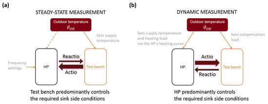
Figure 1.
Methodology of: (a) the steady-state test according to EN 14825; and (b) the dynamic test.
3. Results
3.1. Concept of the Dynamic Method
The dynamic method is based on several individual compensation measurements at different source temperatures (outdoor temperatures ). The individual temperature sequences of the outdoor temperature are combined to form a temperature profile that represents the average (temperate) climate in Europe according to the EN 14825 []. During dynamic testing, the control of the HP (variable frequency drive (VFD) or ON/OFF operation) is active during the whole measurement. The heating capacity is controlled via a compensation load given by the test bench on the sink side. The seasonal performance can be obtained directly via an energy balance.
To determine the seasonal performance according to the dynamic method, the HP is subjected to various conditions on the source side and the sink side. Based on the test conditions given in EN 14825, the conditions on the sink side, the part load ratio (PLR) and the supply temperature , are a function of the outside temperature. Equations (8)–(10), used for our measurements, are based on the linear correlations described in EN 14825. The PLR is defined as the ratio of the heating capacity at outdoor temperatures higher than −10 °C to the nominal heating capacity at the specific outdoor temperature of −10 °C. Further, it is a function of the outdoor temperature according to Equation (8):
The supply temperature for medium temperature level correlates with the outdoor temperature as follows:
The supply temperatures for low temperature level are determined according to Equation (10):
The main criteria for a well-designed test method are representativeness, comparability among different appliances, costs of the measurement and reproducibility []. The outdoor temperature profile for the dynamic test was developed with regard to these criteria as follows:
- The outdoor temperature profile shall represent the average European climate according to the mean occurrence of each temperature from the EN 14825. Therefore, the temperature range of the profile is between −10 °C and 15 °C and the duration of each individual outdoor temperature corresponds to the weighting from the BIN distribution.
- The test duration per temperature sequence shall be chosen to maintain high reproducibility, in particular, for certain operating conditions such as defrost cycles.
- The total test period and the expenses of the dynamic test should be equal or less than the current standard tests.
- The profile should take into account both an increase and a decrease of outdoor temperature and thus reflect the behavior of the HP during changes of the day temperature.
For this study, we chose the duration of each temperature sequence to be at least five hours, which results in total test period of six days (144 h). Figure 2 shows the outdoor temperature profile over the entire test period of six days as well as the supply temperatures and PLRs, the latter two set as a function of the outdoor temperature according to Equations (8)–(10).
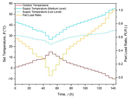
Figure 2.
Profiles of the outdoor temperature (red line), supply temperature at medium (blue solid line) and low level (blue dashed line) and the corresponding part load ratio (yellow line).
3.2. Experimental Data
In this study, we show the results of two HPs tested according to the dynamic method in two different accredited test laboratories (Lab 1 and Lab 2) over the period October 2018 to January 2019. We tested two different methods to provide the outside temperature to the heat pump. For the first method (Lab 1), the heat pump determined the outdoor temperature directly via its temperature sensor, which was installed in a climate box running the outdoor temperature profile shown (see Figure 2). For the second method (Lab 2), the measurement sensors of the heat pump were bypassed by setting the outside temperature by means of a variable electrical resistance. The two methods are examined in Section 3.2.3 with regard to their impact on the HP’s behavior and on the test results. To demonstrate the feasibility of the dynamic method for all types of HPs, we performed tests on both GSHPs and ASHPs. Table 1 gives detailed information about the two test specimen. Both HPs were subjected to the outdoor temperature profile shown in Figure 2. The seasonal performance was calculated according to Equations (5) and (6).

Table 1.
Detailed Information of the HPs tested with the dynamic test method.
During the test, the outdoor temperature, the supply temperature, the heating capacity and the electrical power consumption were recorded with a measurement every ten seconds. Figure 3 exemplarily shows the measurement results of the dynamic test with the climate box for HP#1. For a comparison between measured values and set values, the latter are also shown in Figure 3. On the source side, the measured outdoor temperature (Figure 3a) followed the setpoint values during the entire test period. On the sink side, the supply temperature (Figure 3b) reacted to the variation of the outdoor temperature via the HP’s control according to the correlations, which are given in Equation (9) and depicted in Figure 2. The supply temperature was usually close to the set point values. However, it did not reach the set points at both particularly high and particularly low outdoor temperatures, i.e., at low and at high PLRs. The measured heating capacity (Figure 3c) generally followed the given heating curve, but was on average slightly higher than the set point values, with the exception of the last sequences where PLRs got close to 1. The average heating capacity partly deviated from the set values, especially with particularly low PLRs. The electric power consumption (Figure 3d) increased with increasing heating capacity and vice versa as the HP adjusted the compressor speed to the heating demand continuously via VFD or via ON/OFF operation. Figure 3e shows the cumulated heating energy and the cumulated electric energy consumption. At the end of testing, HP#1 in total provided an amount of heating energy of 711.79 kWh with an electricity consumption of 218.69 kWh. The energy balance resulted in a of 3.25 or rather a seasonal space heating energy efficiency of 122% according to Equations (5) and (6).
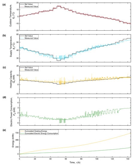
Figure 3.
Results of the dynamic test for HP#1 (GSHP) using the climate box: (a) outdoor temperature ; (b) supply temperature ; (c) heating capacity ; (d) electrical power consumption ; and (e) cumulated energies (thermal and electrical ).
3.2.1. Tests with GSHP
In the following, the behavior under full load conditions (PLR = 1) and part load conditions (PLR = 0.15) is shown for the tested GSHP (HP#1). Figure 4a shows the total of six hours of measurement data acquisition of outdoor temperature, supply temperature, heating capacity and electric power consumption for HP#1 at set outdoor temperatures of −9 °C and −10 °C.
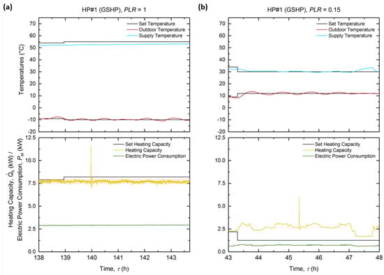
Figure 4.
Measurement of a GSHP using the climate box at: (a) rated capacity (PLR = 1); and (b) part load (PLR = 0.15).
The measured average outdoor temperature corresponded to the required set point temperature at all times. The supply temperature similarly followed the given set point temperature, did does not reach the required values, as it was slightly lower on average than the set point temperature. For an outdoor temperature of −9 °C, the average heating capacity was at the set values, but, for −10 °C, the average heating capacity was again slightly lower than required.
The control behavior of HP#1 at an outdoor temperature of 12 °C (PLR = 0.15) could be deduced from the measurement data curves shown in Figure 4b. Both the average outdoor temperature and the average supply temperature met the required set points. In addition, the temperature curves were continuous and not subject to any fluctuations. The measured heating capacity approached the required heating capacity only during a short phase of approximately one hour and was significantly higher than the set heating capacity for the rest of the temperature sequences. Both the heating capacity and the electric power consumption showed a continuous development. Only temporarily the HP adjusted the heating capacity to approach the set values.
3.2.2. Tests with ASHP
As described in Section 3.2.1, the same six hours of data acquisition at PLRs of 1 and 0.15 are shown for HP#2 (ASHP) in Figure 5. Significant differences in comparison to the data curves of HP#1 (GSHP) shown in Figure 4 can be observed.
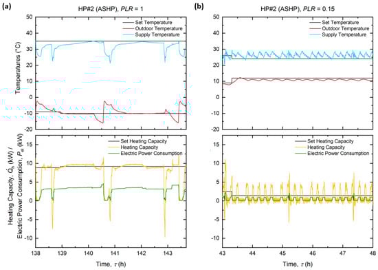
Figure 5.
Measurement of an ASHP using the climate box at: (a) rated capacity (PLR = 1); and (b) part load (PLR = 0.15).
At full load (Figure 5a), a cyclic behavior, caused by defrosting processes at the evaporator, was observed for all measured parameters. The average outdoor temperature provided by the test bench matched the required values. It fluctuated at cyclic intervals as a result of the defrosting phases caused by the HP’s control behavior. The average supply temperature was achieved at some measuring points but was slightly lower on average. The required heating capacity was achieved and provided by HP#2, but the defrosting cycles led to temporary negative heat flows. As a result, the average heating capacity was also lower than the set values. The regulation of the compressor could also be observed by the course of the electric power consumption, especially during defrost cycles.
The measurement data curves of the ASHP (HP#2) in Figure 5b again show considerable differences compared to the measurement data of the GSHP (HP#1) in Figure 4b, since a cyclic behavior was observed for all parameters. The average values of the measured temperatures were higher (supply temperature) or lower (outdoor temperature) than the set temperatures. However, the minima and maxima of the temperature cycles were close to the set values, respectively. The heating capacity fluctuated considerably around the given set value and reached amplitudes of approximately 5–7.5 kW (±200%). The average heating capacity, however, corresponded to the set heating capacity, since the phases with excessively high heating capacity were compensated by phases with no or even negative flow of heating energy. For all parameters, the frequency of the cycles were identical.
3.2.3. Precision of the Dynamic Test Method
The criteria chosen for the design of the dynamic test method are representativeness, comparability among different appliances, costs of the measurement and reproducibility (see Section 3.1). The latter is discussed more in detail in this section with particular focus on the use of the climate box and the electrical resistance. We repeated the dynamic tests for HP#1 and HP#2 in different laboratories. For HP#2, we performed the dynamic test using the climate box twice in the same laboratory (Lab 1) to conclude for repeatability. Figure 6a shows the results of these tests, more precisely the determined cumulative heating energies and cumulative electric energy consumptions.
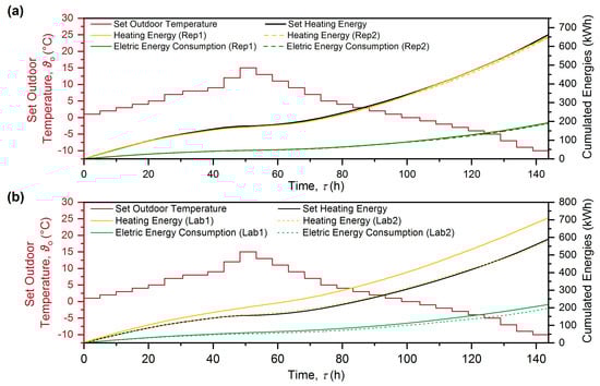
Figure 6.
Cumulated heating energy and cummulated electric energy consumption of: (a) HP#2 measured two times in the same laboratory; and (b) HP#1 measured in different laboratories, Lab 1 and Lab 2, respectively.
The set heating energy represents the ideal case that the heating capacity provided by the HP meets the exact heating demand at all times. HP#2 apparently covered the heating demand almost ideally for both tests, i.e., it neither generated too little nor too much heat. The tests resulted in cumulative heating energies of 650.58 kWh (Lab 1) and 646.96 kWh (Lab 1), respectively. The cumulated electric energy consumption differed only slightly for both measurements, with values of 192.39 kWh and 188.95 kWh, respectively. According to Equations (5) and (6), the cumulated energies resulted in the seasonal space heating energy efficiencies of 132.28% and 133.96%, corresponding to an intra-laboratory precision (repeatability) of 0.63%.
For HP#1, we performed the dynamic test once in two different laboratories to conclude for reproducibility (Lab 1 using the climate box and Lab 2 using the electrical resistance). Figure 6b shows the results of these tests. In both laboratories, the determined electric energy consumptions were similar, with values of 218.69 kWh (Lab 1) and 198.00 kWh (Lab 2), respectively. In contrast, the amount of heating energy produced by HP#1 differed between the two laboratories. As HP#1 strictly followed the heating demand (set heating energy) in Lab 2, it produced excess heat during the tests in Lab 1. According to Equations (5) and (6), the cumulated energies resulted in the seasonal space heating energy efficiencies of HP#1 of 122.20% (Lab 1) and 109.96% (Lab 2), corresponding to an inter-laboratory precision (reproducibility) of 5.01%.
4. Discussion
The dynamic method achieved high repeatability and the inter-laboratory deviation (reproducibility) was at an adequate level. The deviations of the heating energies between Labs 1 and 2 in Figure 6b could be explained by the fact that the set outdoor temperature was assigned to the HP in different ways. In Lab 1, the HP detected the temperature directly via its temperature sensor using the climate box, whereas, in Lab 2, the temperature was given to the HP via an electrical resistance. The test with the electrical resistance implicates that we obtained results, which are independent from the quality of the temperature sensor and thus possible sources of uncertainties, are reduced. Testing using the climate box with the temperature sensor being active, however, enabled recording the control quality of the HP in its entirety. This would be closer to field conditions compared to when using an electrical resistance. In the case of HP#1, for example, Figure 3b,c shows the hysteresis that occurred by comparing set point and actual values of the sink side parameters at low and high outdoor temperatures (low and high PLRs). This could occur because the outdoor temperature detected by the HP differed from the actual outdoor temperature. Most likely, the reproducibility can be further improved using the same methods to provide the outdoor temperatures (via electrical resistance or via climatic box). Furthermore, from the test results, a continuous behavior, even during ON/OFF-operation, was observed (see Figure 5b) and thus the test duration could be significantly shortened without losing precision.
The comparability of various HPs could be a significant advantage of the dynamic method in comparison to current standards such as EN 14825. Figure 7 shows the heating capacity of five HPs, determined according to EN 14825, and the demanded heating load (set value) required for the respective outdoor temperatures.
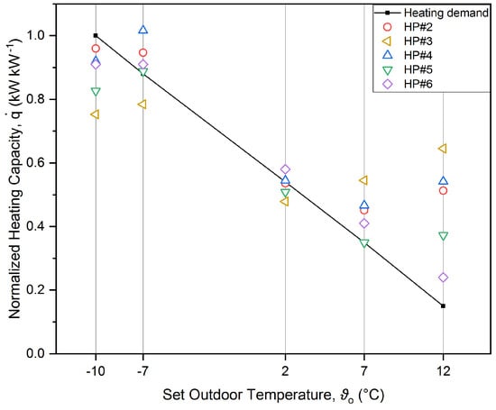
Figure 7.
Average heating capacity determined according to EN 14825 (fixed compressor speed) of several HPs, including HP#2.
Although these HPs were all tested at fixed compressor speeds according to the manufacturers’ instructions, they could not meet the required heating capacity for most of the tested operating points. At low outside temperatures, HP#3 and HP#5 could not achieve the required heating capacity within the permissible deviations according to EN 14825 (±10%). This is due to the HPs’ specification of the bivalence temperature. Below this particular temperature, the HPs cannot provide the amount of demanded heating capacity by themselves and thus would need additional support by an electric heater in the field. In our case, we observed bivalence temperatures at 2 °C (HP#3) and −7 °C (HP#5). At higher outside temperatures, all HPs generally provide higher heating capacities than required. The deviations at outdoor temperatures of 7 °C and 12 °C can be directly attributed to the methodology of EN 14825. According to the EN 14825, the supply temperature is increased whenever ON/OFF operation would occur, thus circumventing OFF-sequences. This consequently results in an increase of heating capacity. If the heating capacity is more than 10% higher than demanded, the EN 14825 requires adjusting the coefficient of performance (COP) with prescribed correction factors. (According to EN 14825, the prescribed correction factors are and . is the ratio of measured heating capacity and required heating capacity. The degredation coefficient is determined via the formula for each PLR, respectively. is the electric power consumption measured during 5 min after the compressor has been switched off for 10 min and is the electric power consumption during operation at a particular PLR. generally achieves values of between 0.9 and 1.)
Figure 8a shows the comparison of the heating capacities of HP#2 for different outdoor temperatures, determined with the dynamic method (unfixed compressor speed) and with the standard method EN 14825 (fixed compressor speed).
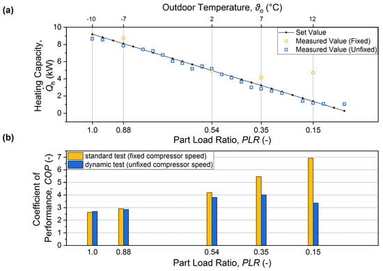
Figure 8.
(a) Average heating capacity; and (b) Coefficient of Performance results of HP#2 for different PLRs determined with the dynamic method (unfixed compressor speed: VFD or ON/OFF operation) and according to EN 14825 (fixed compressor speed).
At PLRs higher than 0.54, the HP operated with variable compressor speed during the dynamic test. For PLRs lower than 0.54, we observed ON/OFF operation. The heating capacities of the dynamic method are the average values of the entire respective temperature sequence, including the periods of OFF operation and the stabilization phase at the beginning of each sequence. The consideration of the stabilization phase is permissible as the small fluctuations during the stabilization phase can be neglected. It is shown that the heating capacities determined with the dynamic method are close to the demanded heating load, whereas in the standard test an excessive heat can be observed at low PLRs due to the aforementioned methodology of EN 14825. Figure 8b shows the corresponding COPs for the dynamic method and for the standard method EN 14825 (after applying the correction factors). The COP determined with EN 14825 increases continuously with decreasing PLR, whereas the COP determined with the dynamic method also increases initially with decreasing PLR, but decreases again as soon as ON/OFF operation occurs. (According to EN 14825, after applying the correction factors, the is called . However, for reasons of simplicity, we call the coefficient of performance simply for both methods.) The high deviations of COPs between standard test and dynamic test at low PLRs might indicate that the efficiency losses due to ON/OFF operation are not adequately taken into account by the correction factors. Thus, the methodology of the EN 14825 could lead to an overestimation of the COP at low PLRs. In addition, the standard test loses comparability between different HPs because the adjustment of the supply temperature is individual for each HP, respectively (see Figure 7). In contrast, the dynamic method provides both, the consideration of efficiency losses during ON/OFF operation and a comparability for various HPs without the need for correction factors.
The performed tests showed that the dynamic method can be applied to both HP types, GSHPs and ASHPs, with common modifications to the test bench (see Section 2).
The control of an HP is its individual strategy to reach the requirements on the sink side via its heating curve and is taken into account by applying the dynamic test method. It was observed that the HPs were usually unable to meet the heating set points for PLRs close to 1 and 0. However, particularly in these cases, the dynamic method enables a clear differentiation between the control behaviors of tested HPs in the case of using the climate box. For PLR = 1, for example, HP#1 does not provide a sufficient amount of heat, but for PLR = 0.15, in contrast, it generates a slight excess of heat. HP#2, on the other hand, is able to meet the required heating capacity precisely. The dynamic method, however, provides a fair comparison of HPs with different control strategies. It should be put up for discussion if tested HPs should in any case achieve the setup values on the sink side for reasons of comparability. In this context, the two methods, climate box and electrical resistance, should be further examined.
5. Conclusions
The growing market penetration of HPs indicates the need for a performance test method that better reflects their capacity modulation. Currently, energy efficiency testing for HPs is only executed in particular test modes that fix the compressor speed and do not reflect the real use behavior of HPs. This study proposes a test method with dynamic profiles based on climate data and designed for outside temperature, supply temperature and the heating capacity. The dynamic test method has the following advantages:
- It considers the real control behavior of HPs.
- It can be conducted independently from manufacturer support and makes special test modes obsolete.
- It considers the whole temperature range of a heating season (from −10 °C to 15 °C for average European climate) directly by measurement, specifically those sequences that are commonly linearly interpolated in current standards.
- It makes linear interpolation and the prescription of invariables obsolete and hence gives a closer approximation of the field performance of HPs and could reduce the need for field tests.
- It has the potential to achieve a high degree of automation and could be easily modified to new technologies.
Furthermore, based on these findings, we propose that the following should be subject to further research:
- The optimum values for the permitted deviations and tolerances are to be defined.
- The temperature sequences can be further shortened. Therefore, the influence of the stabilization phase on the average results should be investigated for all temperature sequences.
- The feasibility for testing fixed-speed HPs should be investigated.
- The use of climate box and electrical resistance should be examined.
Author Contributions
Conceptualization, C.P.; methodology, C.P. and A.Z.; software, A.Z. and I.M.; validation, C.P., A.Z. and I.M.; formal analysis, C.P.; investigation, A.Z. and I.M.; resources, A.S.; data curation, C.P.; writing—original draft preparation, C.P.; writing—review and editing, A.Z., I.M. and A.S; visualization, C.P.; supervision, A.S.; and project administration, A.S.
Funding
This research received no external funding.
Acknowledgments
This project was financed as a part of the National Action Plan on Energy Efficiency (NAPE) of the German Federal Ministry for Economic Affairs and Energy.
Conflicts of Interest
The authors declare no conflict of interest.
Abbreviations
The following abbreviations are used in this manuscript:
| ASHP | air source heat pump |
| GSHP | ground source heat pump |
| COP | coefficient of performance |
| HiL | Hardware-in-the-Loop |
| HP | heat pump |
| PLR | part load ratio |
| SCOP | seasonal coefficient of performance |
| VFD | variable frequency drive |
Appendix A
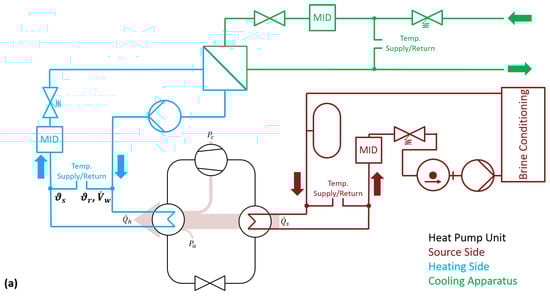
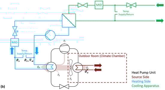
Figure A1.
Experimental Setup for: (a) GSHP; and (b) ASHP applications.
References
- Chua, K.J.; Chou, S.K.; Yang, W.M.; Yan, J. Achieving better energy-efficient air conditioning—A review of technologies and strategies. Appl. Energy 2013, 104, 87–104. [Google Scholar] [CrossRef]
- Heat Roadmap Europe 2050. Heating and Cooling Facts and Figures—The Transformation towards a Low-Carbon Heating & Cooling Sector. Heat Roadmap Europe, 2017. Available online: https://www.isi.fraunhofer.de/content/dam/isi/dokumente/cce/2017/29882_Brochure_Heating-and-Cooling_web.pdf (accessed on 18 March 2019).
- Berardi, U. A cross-country comparison of the building energy consumptions and their trends. Resour. Conserv. Recyl. 2017, 123, 230–241. [Google Scholar] [CrossRef]
- Connolly, D.; Lund, H.; Mathiesen, B.V. Smart energy Europe: The technical and economic impact of one potential 100% renewable energy scenario for the European Union. Renew. Sustain. Energy Rev. 2016, 60, 1634–1653. [Google Scholar] [CrossRef]
- Mathiesen, B.V.; Lund, H.; Karlsson, K. 100% renewable energy systems, climate mitigation and economic growth. Appl. Energy 2011, 88, 488–501. [Google Scholar] [CrossRef]
- Li, G. Investigations of life cycle climate performance and material life cycle assessment of packaged air conditioners for residential application. Sustain. Energy Tech. Assess 2015, 11, 114–125. [Google Scholar] [CrossRef]
- Shao, S.; Shi, W.; Li, X.; Chen, H. Performance representation of variable-speed compressor for inverter air conditioners based on experimental data. Int. J. Refrig. 2004, 27, 805–815. [Google Scholar] [CrossRef]
- Tu, Q.; Zhang, L.; Cai, W.; Guo, X.; Yuan, X.; Deng, C.; Zhang, J. Control strategy of compressor and sub-cooler in variable refrigerant flow air conditioning system for high EER and comfortable indoor environment. Appl. Therm. Eng. 2018, 141, 215–225. [Google Scholar] [CrossRef]
- Choi, J.M.; Kim, Y.C. Capacity modulation of an inverter-driven multi-air conditioner using electronic expansion valves. Energy 2003, 28, 141–155. [Google Scholar] [CrossRef]
- Jeong, K.; Choi, J.M. Capacity modulation of a cascade heat pump with the variation of compressor speed and electronic expansion valve opening. Renew. Sustain. Energy 2014, 6, 053107. [Google Scholar] [CrossRef]
- Park, Y.C.; ChulKim, Y.; Min, M.-K. Performance analysis on a multi-type inverter air conditioner. Energy Convers. Manag. 2000, 42, 1607–1621. [Google Scholar] [CrossRef]
- Chen, W.; Zhou, X.; Deng, S. Development of control method and dynamic model for multi evaporator air conditioners (MEAC). Energy Convers. Manag. 2005, 46, 451–465. [Google Scholar]
- DIN Normenausschuss Kältetechnik (FNKä). DIN EN 14825:2016 Air Conditioners, Liquid Chilling Packages and Heat Pumps, with Electrically Driven Compressors, for Space Heating and Cooling—Testing and Rating at Part Load Conditions and Calculation of Seasonal Performance; DIN Normenausschuss Kältetechnik (FNKä): Berlin, Germany, 2016. [Google Scholar]
- Standards Australia and New Zealand Standards. AS/NZS 3823:2014 Performance of Electrical Appliances—Air Conditioners and Heat Pumps; Standards Australia and New Zealand Standards: Sydney, Australia; Wellington, New Zealand, 2014. [Google Scholar]
- Air Conditioning, Heating and Refrigeration Institute. ANSI/AHRI 210/240:2008. Standard for Performance Rating of Unitary Air-Conditioning & Air-Source Heat Pump Equipment; Air Conditioning, Heating and Refrigeration Institute: Arlington, VA, USA, 2008. [Google Scholar]
- American Society of Heating, Refrigerating and Air-Conditioning Engineers Inc. ASHRAE, ANSI/ASHRAE Standard 116-2010 Methods of Testing for Rating Seasonal Efficiency of Unitary Air Conditioners and Heat Pumps; American Society of Heating, Refrigerating and Air-Conditioning Engineers Inc.: Atlanta, GA, USA, 2010. [Google Scholar]
- Japanese Industrial Standards Committee. JIS C9612: 2013 Room Air Conditioners; Japanese Industrial Standards Committee: Tokyo, Japan, 2013. [Google Scholar]
- Gomes, A.; Antunes, C.H.; Martinho, J. A physically-based model for simulating inverter type air conditioners/heat pumps. Energy 2013, 50, 110–119. [Google Scholar] [CrossRef]
- Cuevas, C.; Lebrun, J. Testing and modelling of a variable speed scroll compressor. Appl. Therm. Eng. 2009, 29, 469–478. [Google Scholar] [CrossRef]
- Lee, S.H.; Jeon, Y.; Chung, H.J.; Cho, W.; Kim, Y. Simulation-based optimization of heating and cooling seasonal performances of an air-to-air heat pump considering operating and design parameters using genetic algorithm. Appl. Therm. Eng. 2018, 144, 362–370. [Google Scholar] [CrossRef]
- Menegon, D.; Soppelsa, A.; Fedrizzi, R. Development of a new dynamic test procedure for the laboratory characterization of a whole heating and cooling system. Appl. Energy 2017, 205, 976–990. [Google Scholar] [CrossRef]
- Haller, M.Y. Dynamic whole system testing of combined renewable heating systems - The current state of the art. Energy Build. 2013, 66, 667–677. [Google Scholar] [CrossRef]
- Riederer, P.; Partenay, V.; Raguideau, O. Dynamic test method for the determination of the global seasonal performance factor of heat pumps used for heating cooling and domestic hot water preparation. In Proceedings of the 11th International IBPSA Conference, Glasgow, UK, 27–30 July 2009. [Google Scholar]
- Huchtemann, K.; Engel, H.; Mehrfeld, P.; Nürenberg, M.; Mueller, D. Testing method for evaluation of a realistic seasonal performance of heat pump heating systems: Determination of typical days. In Proceedings of the 12th REHVA World Congress, Aalborg, Denmark, 22–25 May 2016. [Google Scholar]
- Mavuri, S. Field behaviour of inverter air conditioners effect on seasonal performance. IJAIEM 2015, 4, 18–25. [Google Scholar]
- Grote, K.H.; Feldhusen, J. Thermodynamik. In Dubbel-Taschenbuch fuer den Maschinenbau; Springer: Berlin/Heidelberg, Germany; New York, NY, USA, 2005; p. D45. [Google Scholar]
- European Commission. Commission Delegated Regulation (EU) No 811/2013. Off. J. Eur. Union 2013, L289, 136–161. [Google Scholar]
- Meier, A.K.; Hill, J.E. Energy test procedures for appliances. Energy Build. 1997, 26, 23–33. [Google Scholar] [CrossRef]
© 2019 by the authors. Licensee MDPI, Basel, Switzerland. This article is an open access article distributed under the terms and conditions of the Creative Commons Attribution (CC BY) license (http://creativecommons.org/licenses/by/4.0/).