On-Coupling Mechanical, Electrical and Thermal Behavior of Submarine Power Phases

Abstract

Floating offshore renewable energies (OREs), such as offshore floating wind turbines (wind energy) or wave power (wave and wave energy), are increasingly in demand. Submarine cables that transmit the energy produced from offshore farms all the way to onshore stations are critical structures that must be able to work perfectly over 20 years without any maintenance. In order to reduce the significant costs associated with electrical cables, it is important to optimize the dimensioning of the components of these cables, or to develop structural monitoring techniques that target zero and/or minimum maintenance over their lifespan. In this paper, we FEM of the impact of damage mechanisms of the conductor part of a submarine power phase on its mechanical, electrical, and thermal behavior. The main damage mechanisms are local plasticity and wire failure. The first mechanical study made it possible to obtain the elasto-plastic behavior of the conductor. The electrical study took into consideration the deformed geometry of the conductor in the elasto-plastic domain, as well as the non-homogeneous distribution of the electrical conductivity of the conductor. Their influence on the electrical resistance of the conductor was then analyzed. Finally, we studied the impact of plasticity and conductor failure on the thermal behavior of the phase. The temperature differences obtained in the numerical analysis of this work may be used further to help preventive and curative maintenance of the cables, for example, by using an optical fiber as sensor for structural health monitoring.

1. Introduction

Marine renewable energy (MRE) is one of the most promising sources of clean energy and is part of the European energy strategy. The connection of MRE offshore farms to onshore stations requires the use of reliable power dynamic and static cables for energy transport. Previous work and projects have been devoted to this topic [1,2,3] and have concentrated solely on mechanical behavior or, else, on thermal behavior and/or electrical behavior. However, the conductor part is a metal and it is crucial to establish a multiphysical model that can link mechanical, thermal, and electrical behavior together. A submarine cable is subject to severe mechanical stresses (tension, compression, flexion, and torsion) during manufacture, handling, transportation, installation, and operation [4]. These stresses can affect the overall mechanical and physical properties of the conductor. Indeed, the conductor wires are subject to tensile and torsional forces, compressive forces, and tangential forces generated by the friction between the wires. As the wires, in general, are made of copper—which is a weak metal—these stresses gradually generate plasticity, and then result in failure (Figure 1). This plastic deformation is due to the formation, multiplication, and displacement of moving linear defects in the crystal lattice of the metal, called dislocations. Furthermore, additional post-plasticity defects in the crystal lattice of the metal progressively decrease both electrical and thermal transport [5]. The movement and creation of dislocations, therefore, change the mechanical behavior of the metallic material, as well as its physical properties (e.g., electrical, thermal, etc.) [6].

Due to the geometric complexity (e.g., mesh generation, calculation cost, etc.) of a submarine power cable, most of the mechanical models available in the literature are based on analytical solutions. Analytical models [7,8,9] were developed following the context of “material resistance” of linear beam theory, and are based on slender beam models. These models are used to determine the axial behavior of the cable and its bending behavior, and have the advantage of providing approximate estimates of stiffness terms (traction, torsion, and bending) from a limited amount of input data: geometry of the cable cross-section, material properties, and loads. However, their scope of validity remains limited. In the literature [10], it has been shown that these analytical solutions remain valid for a strand lay angle below 20°. In addition, most of these models focus on longitudinal axial stress, thus neglecting shear stresses. It is worthwhile to note that these analytical models, which were developed for steel cables, can hardly be applied to copper due to its lack of mechanical performance.

In addition to analytical models, other work focused on finite element modeling (FEM) has been carried out with a limited success and some issues raised. Indeed, meshing problems resulting from geometric complexity, as well as non-linearity resulting from inter-wire contacts, were shown to be the main issues facing implementation of numerical models. The resulting models used heavy calculation, which is very time-consuming. To avoid extensive calculation, available numerical models only simulate a short portion of the pitch length of the cable, particularly for single-layer cables (1 + 6) [2,3,4,5].

The aim of this paper was to use numerical modeling to study the impact of damage mechanisms on the mechanical, electrical, and thermal properties of a submarine power phase. The models were developed using COMSOL Multiphysics®. The originality of our work comprised modeling a multilayer conductor (1 + 6 + 12) with a significant length of one meter and the elasto-plastic behavior of copper, as well as the multiphysical aspect that includes electrical and thermal behaviors. The performance of submarine high-voltage cables must be studied from a multiphysics point of view, as not only do multiphysics parameters play a key role simultaneously, but also chemical and environmental aspects (e.g., humidity, salt, corrosion-assisted fatigue, etc.). As will be seen later in this work, our results are confirming the validity of this strategy.

This paper is organized as follows. In Section 2, the design of the cable used in the simulations is briefly presented, as well as the description of the different physical models. Then, the mechanical model to determine the plastic response of the conductor under tension is detailed. The deformed geometry and non-homogeneous distribution of electrical conductivity due to strain hardening have been used in the electrical model. The conductor was subjected to a potential difference in order to calculate its electrical resistance. For thermal modeling, the two-dimensional thermal model described the thermal behavior of the phase resulting from the plasticity of the conductor and the failure of the strands. The results of our models, analysis, and comments are presented in Section 3.

2. Multiphysical Power Phase Models

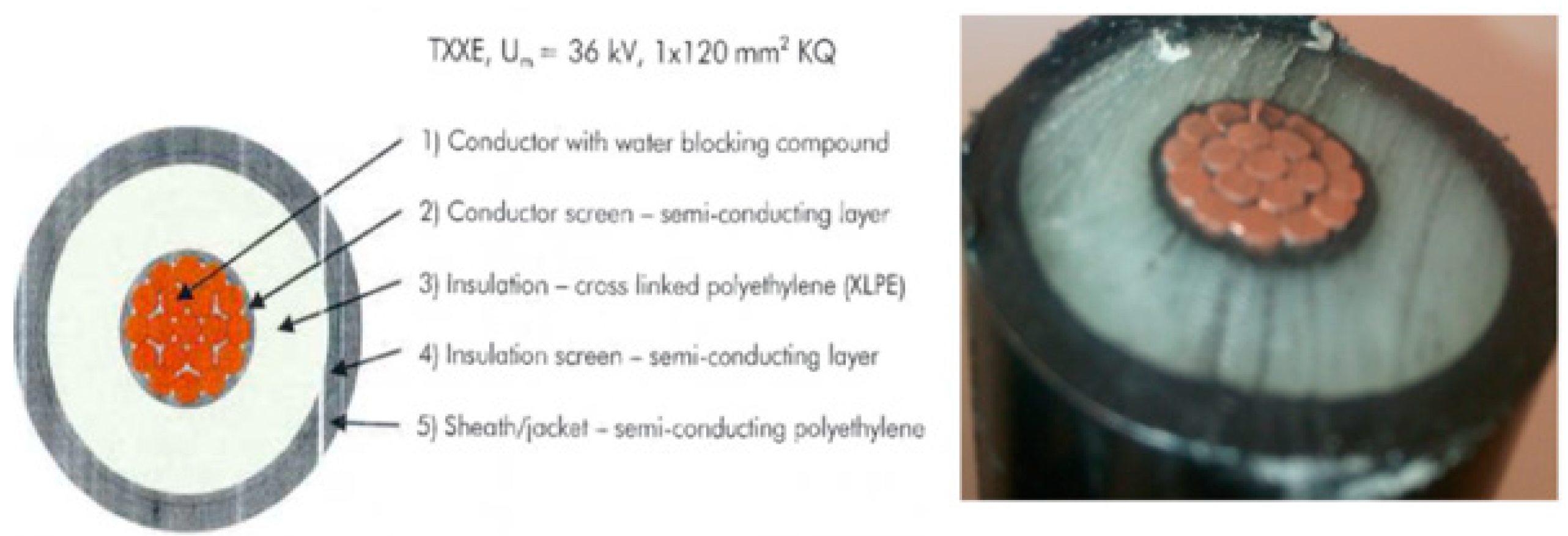
2.1. Cable Design and Characteristics

The cable targeted by these simulations was a power cable phase with synthetic insulation (XLPE, 36 kV). The conductor was made of copper with a cross-section of 120 mm². The structure of the cable cross-section is shown in Figure 2. The thermal and mechanical properties for each material used in the cable design are presented in

Table 1. Thermal and mechanical properties of cable components [8].

Component	Material	Thermal Conductivity (W∙K−1∙m−1)	Heath Capacity (MJ∙m−3 K−1)	Young’s Modulus (GPa)	Poisson’s Ratio
Conductor	Copper (Cu)	370.40	3.45	112	0.30
Conductor Screen	Semiconducting polymer	0.50	2.40	0.34	0.34
Insulation	Crosslinked polyethylene (XLPE)	0.28	2.40	0.35	0.40
Insulation Screen	Semiconducting polymer	0.50	2.40	0.34	0.34
Sheath	Polyethylene (PE)	0.20	1.70	0.34	0.40

. These values were taken from the standard IEC 60287 [11].

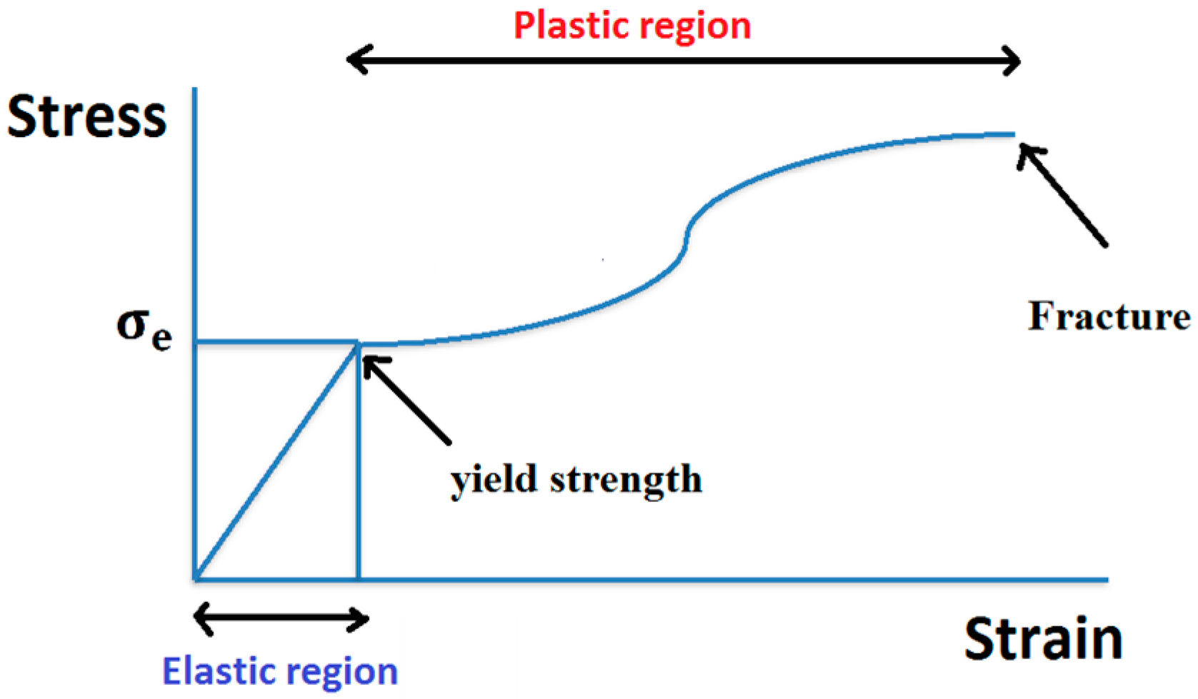
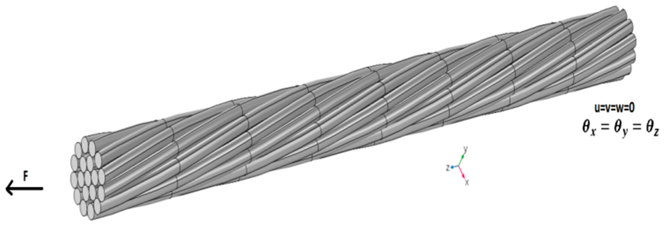
2.2. Mechanical Model

Firstly, at this stage, we built a mechanical model of a submarine power phase conductor (1 + 6 + 12) (Figure 3). The model comprised a three-layered straight strand made from a central straight wire and two outers layers—composed by 6 and 12 wires helically wrapped around the central wire, respectively. All wires had the same radius, and the overall length of the wire phase model was 1 m. A model was created using COMSOL Multiphysics^®.

The model simulated tensile behavior of a submarine power phase, which allowed us to compute the distribution of mechanical stresses and conductor deformation. To quantify the states of stress and strain in the conductor by FEA, it was necessary to describe the behavior of the material using a mechanical model. The equilibrium equations were based on Newton’s second law. In terms of stresses, it can be formulated as follows [12]:

$$div\left(\sigma \right)=f ,$$

(1)

with $\sigma$ being the stress tensor and $f$ representing all external forces. The material induced strains in the system are expressed as

$${\epsilon }_{tot}={\epsilon }_e+{\epsilon }_p ,$$

(2)

where the total strain ${\epsilon }_{tot}$ is a combination of elastic ${\epsilon }_e$ and plastic ${\epsilon }_p$ strains. The elastic strain follows Hook’s law:

$$\sigma =C:\left({\epsilon }_e\right) .$$

(3)

Combining Equations (2) and (3), the stress–strain relationship for a material can be expressed as

$$\sigma =C:\left( {\epsilon }_{tot}-{\epsilon }_p\right) .$$

(4)

This model was completed by boundary conditions, such as imposed displacements and loading (Figure 3). All degrees of freedom (translation and rotation) in the section (z = 0) were constrained. At the other end (z = L) they were restrained so as not to rotate in all three directions and not to displace in x and y directions, considering monotonous loading was applied in the z direction.

All wires were made of homogeneous and isotropic material copper. The cable was studied using considered elasto-plastic material models with a linear isotropic hardening case. The elastic domain is governed by Young’s modulus and Poisson’s ratio. The yield stress of copper was ${\sigma }_e$ = 135 MPa and the plastic domain was based on tensile experiment of a single conductor [2]. The results of the tensile test are presented in

Table 2. True stress and plastic strain.

True Stress (MPa)	Plastic Strain (1)
135	0
144.49	0.01
159.94	0.019
179.43	0.036
200.38	0.06
213.5	0.07
230.5	0.01
243.36	0.11
256.98	0.13
266.41	0.15
279.25	0.16
285.01	0.18
306.45	0.21
316.75	0.24
328.69	0.28
340.76	0.29

.

Some articles show that contact hypotheses have a negligible influence on the overall tensile behavior of the cable [13]. Therefore, the hypothesis of friction between the wires of the conductor was not taken into account. In this model, tetrahedral meshes were used to subdivide the power cable and, to improve the computing precision and obtain a better convergence, the uneven mesh generation was adopted. Each node had three translational degrees of freedom in x, y, and z directions.

2.3. Electrical Model of the Conductor

DC electrical simulations were made using the electrical module of COMSOL software. The DC electrical model was governed by Maxwell’s equations [14]:

$$\{\begin{array}{c}div\left(J\right)=0\\ J=\sigma E+J_e \\ E=-\nabla V\end{array},$$

(5)

where J(A/m²) is the current density, E(v/m) is the electrical field intensity, V(v) is the electrical potential, σ(S/m) is the electrical conductivity of the material, and $J_e$is the externally generated current density.

The model developed was based on exposure of the deformed structure—obtained by the mechanical study—to an electrical potential difference between the two extreme surfaces of the conductor. We also considered the impact of hardening on the electrical conductivity of the material. Therefore, we introduced an experimental behavior law [5] obtained for a copper wire, coupling electrical conductivity and mechanical stresses (Figure 4). This characteristic made it possible to control the evolution of electrical conductivity according to the distribution of the stress resulting from mechanical calculation.

Computation of the current intensity (I) in the of conductor was obtained by making the cut plane 2D at the middle cross-section of the cable and using the surface integral over current density ($J_z$) along the z-axis.

$$I={{\displaystyle \iint }}^{ }{J}_{z}ds$$

(6)

The electrical resistance of the conductor can be calculated by Ohm’s law: $R=\frac{\Delta V}{I}$.

2.4. Thermoelectric Model of the Phase

The main objective of thermal sizing of a cable was to transmit the maximum current without the conductor temperature exceeding the degradation temperature of the XLPE insulation (90 °C). At this stage, we built a thermal model to understand the impact of mechanical effects (plasticity) and strand failure on the thermal behavior of the phase. For calculation cost considerations, only a 2D model was developed.

The equation of heat transfer by steady state conduction, taking into account the thermoelectric coupling [15], was defined as follows:

$$div\left(-K\nabla T\right)=\sigma .{\left|\nabla V\right|}^2$$

(7)

where T is the temperature (K), $K$ is the thermal conductivity (W∙m⁻¹∙K⁻¹), V is the electrical potential (v), and σ(S/m) is the electrical conductivity of the material—which is given by the formula:

$$\sigma =\frac{L}{R.A}$$

(8)

with R as the resistance of the conductor, A as the total surface area of the conductor strands, and L as the length of the strand.

On the cable surface, natural convection and heat radiation were considered, and the corresponding boundary conditions can be described as follows:

$$-\nabla \left(KT\right).n=h\left(T_{ext}-T\right)$$

(9)

where h is the convective heat transfer coefficient, and $T_{ext}$ the ambient temperature. The coefficient h at the surface is given by the formula $h=\frac{k.Nu}{L}$ where L is the diameter of the cable, k is the thermal conductivity of the surrounding environment, and Nu is the Nusselt number. In natural convection, and for a cable laid horizontally, the Nusselt number is given by the following formula [16]:

$$Nu={\left[0.6+\frac{0.387R_a^{1/6}}{{\left[1+{\left(\frac{0.559}{P_r}\right)}^{9/16}\right]}^{8/27}}\right]}^2$$

(10)

According to the Stefan–Boltzmann law, the heat radiation on the cable surface can be described as

$$-\nabla \left(KT\right).n=\epsilon \nu \left(T_{ext}^4-T^4\right)$$

(11)

where ε is the emissivity of the material and is 0.9, and ν is the Stefan–Boltzmann constant.

3. Results and Discussion

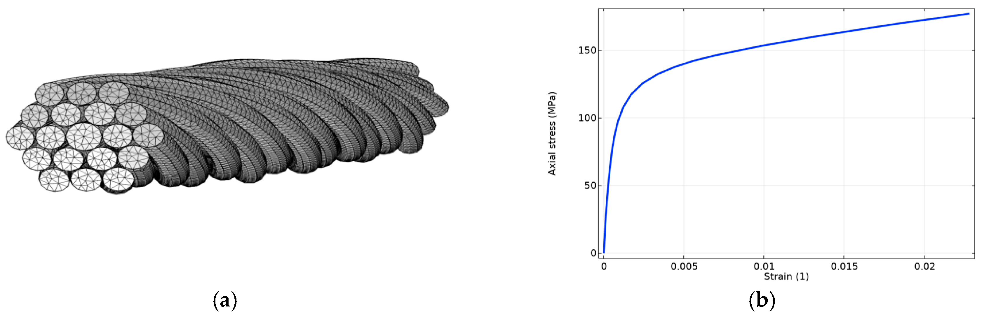
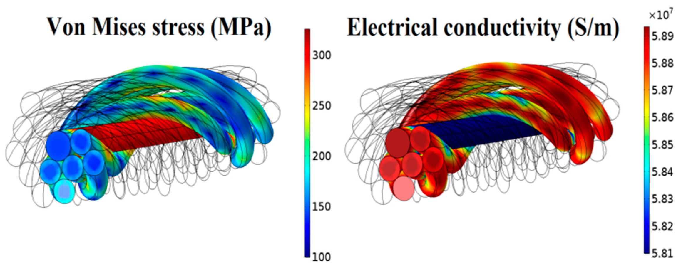
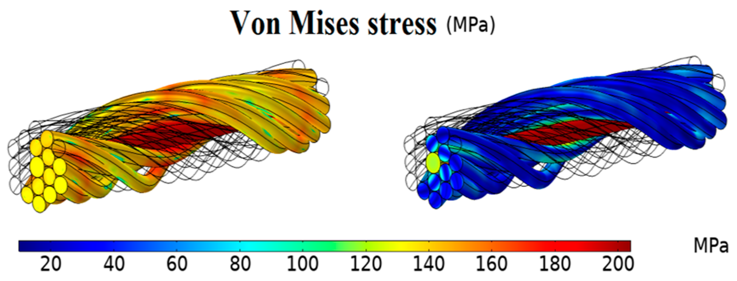
3.1. Results of the Mechanical Model

Figure 5a shows the mesh used for the mechanical model of the conductor (1 + 6 + 12). The mesh had 14,536 nodes for 54,252 elements. To analyze the results obtained, we calculated von Mises stress (12) to position itself with respect to the yield strength ${\sigma }_e$. The distribution of von Mises stress is shown in Figure 6. From this figure, we can see that the stresses were significant at the level of the central wire, as well as at the contact areas between the central wire and the helical wires. Therefore, the central wire and the wires of the first layer were more susceptible to yielding first.

These results support those obtained for a monolayer conductor (1 + 6) [2,3]. Also, the stress–strain curve of the conductor was completely simulated and is displayed in Figure 5b.

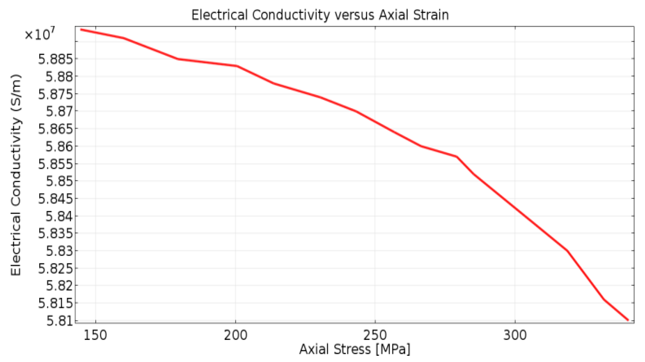
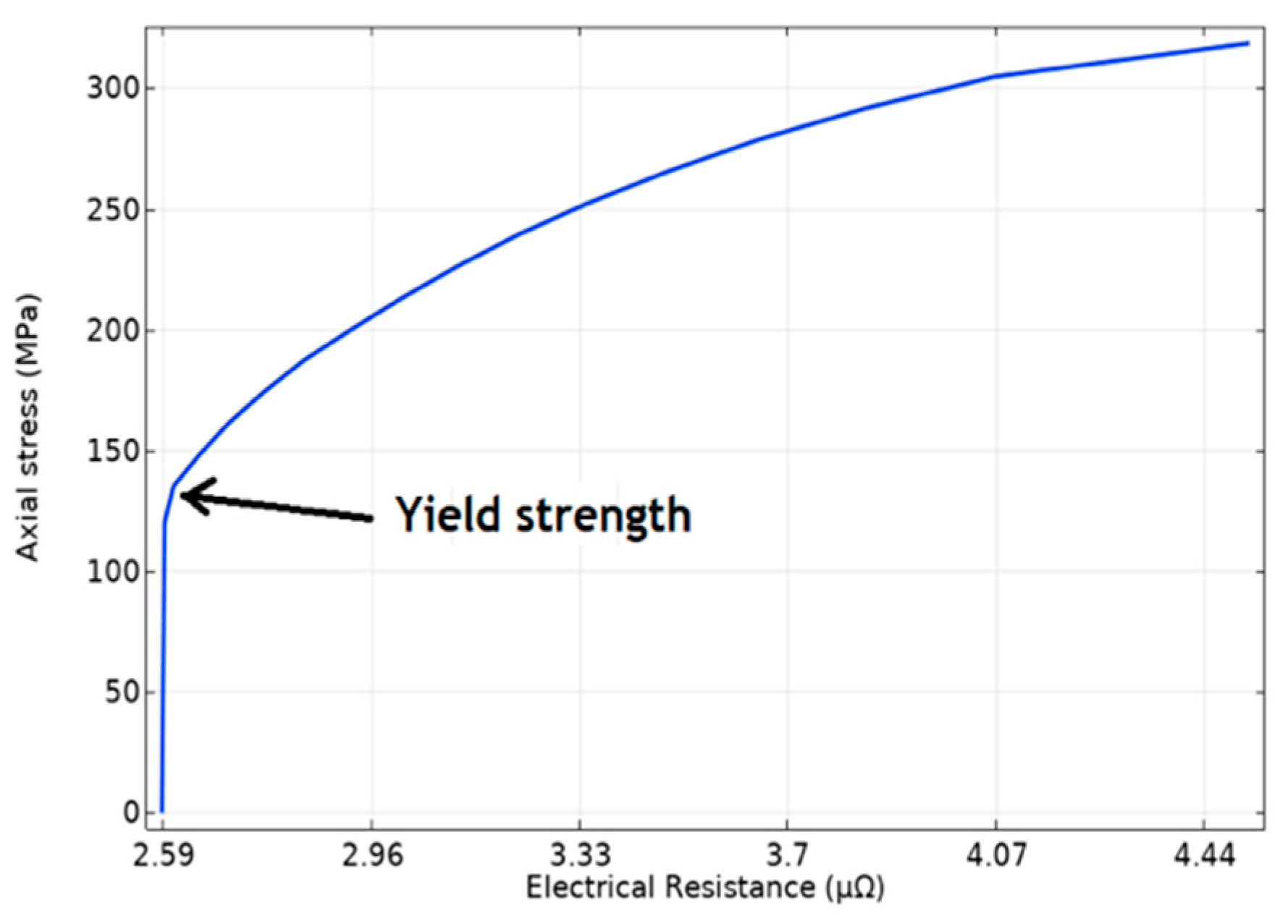
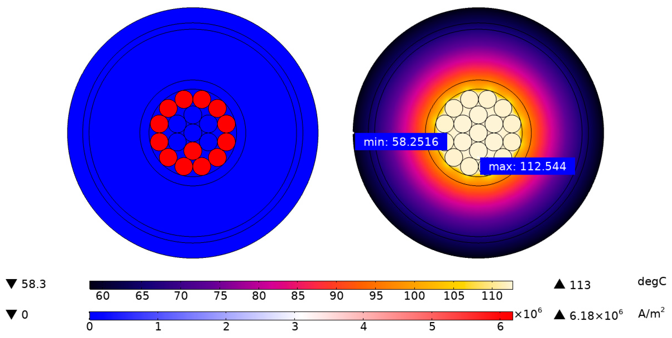
3.2. Results of the Electrical Model

Figure 7 shows the distribution of von Mises stress in the conductor in the plastic range and its correspondence with electrical conductivity. It was shown that electrical conductivity was lower in areas where mechanical stress was greater. This means that these areas become less conductive when stressed, and thus damage accumulates.

Figure 8 shows the evolution of the axial stress as a function of the total electrical resistance of the conductor. We observed that the resistance was almost constant in the elastic area. In the plasticity area, an increasing evolution of electrical resistance was observed. For 200 MPa, which corresponds to 120% of the yield strength, we observed a 14% increase in resistance (∆R/R). The shape of this curve is in agreement with that obtained in [6] for a single strand of aluminum. This result can be considered, therefore, as an electrical loading curve, analogous to the mechanical stress–strain curve where we can clearly visualize the “elastic” electrical area and the “plastic” one.

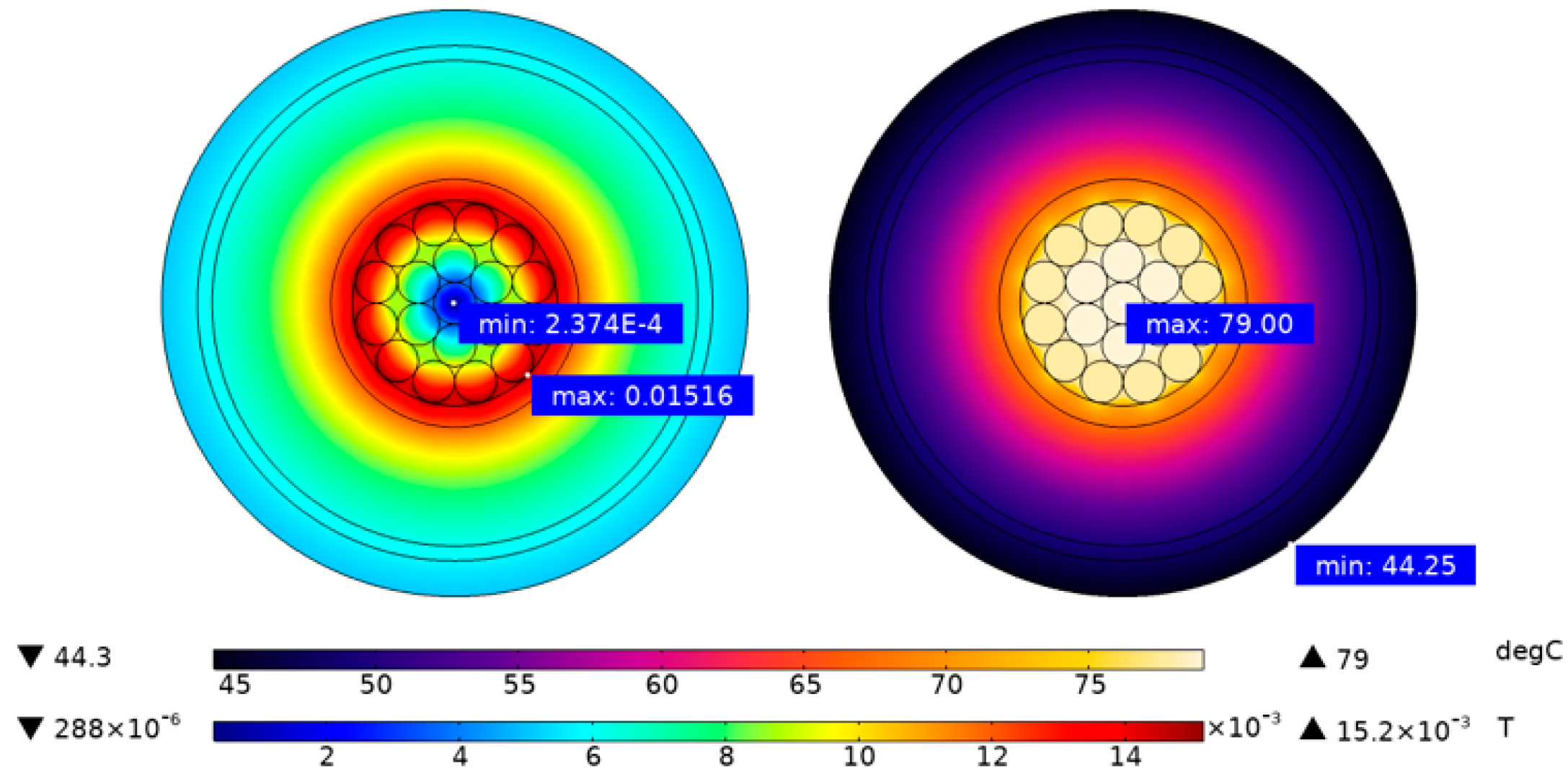
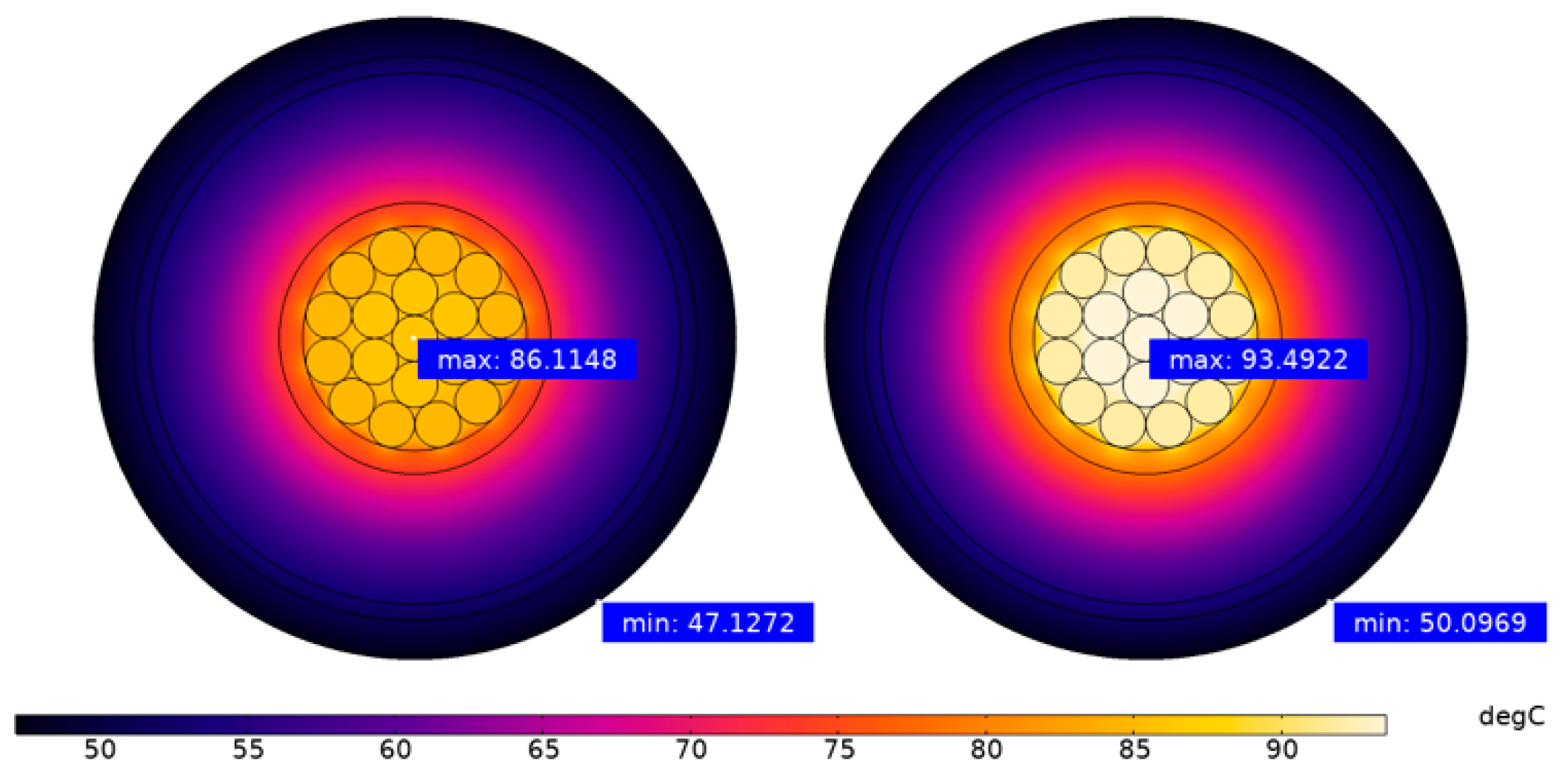
3.3. Results of the Thermoelectric Model

As was shown in Figure 8a, the axial stress was calculated as a function of thermal resistance and the result is shown in Figure 8b. It is interesting to note that the envelopes of stress–strain, axial stress–electrical resistance, and axial stress–thermal resistance are identical. This implies that damage accumulation—which affects mechanical performance of a conductor—also affects electrical and thermal resistance with equivalent magnitude. This result can significantly help to check the status of a high-voltage cable prior to placement in deep-sea. Indeed, checking for damage on samples at the end of the manufacturing process and/or after shipping operations can help identify the magnitude of damage accumulation and, thus, the effect on electrical and thermal performances of cables. This identification can then ease the final decision of placement, or not, in deep-sea.

The phase was considered to be laid horizontally in the free air with an ambient temperature of 20 °C. The value for the convective heat transfer coefficient h was 11 (W/m²∙K). At first, it was assumed that the cable had not been damaged mechanically. Figure 9 shows the temperature distribution and the magnetic field when the conductor was carrying a current of 500 A. This result serves as a reference for the next stage.

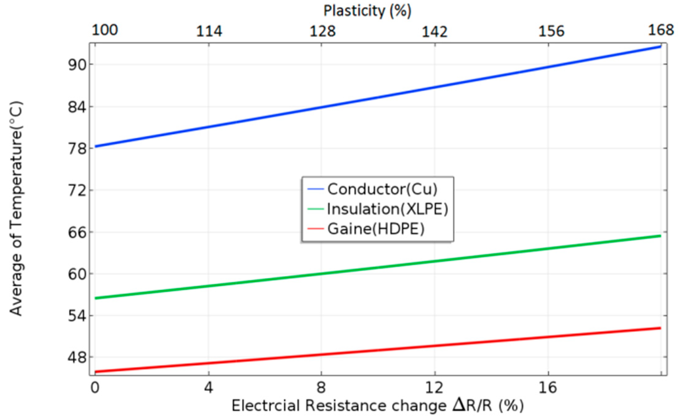
3.4. Plasticity Effect on the Thermal Behavior of the Phase

The objective of this stage was to study the thermal sensitivity of the cable to the different levels of conductor plasticity (100%${\sigma }_e$, 110%${\sigma }_e$; Figure 1). The coupling of thermal behavior to plasticity is represented by the curve in Figure 8—linking mechanical stresses to electrical resistance—and Equation (8)—linking electrical resistance to electrical conductivity. For each stress level, the corresponding electrical conductivity can be calculated. Finally, we inserted this last conductivity value into Equation (4) to calculate temperatures that were encountered. Figure 10 shows the impact of plasticity on the thermal behavior of the cable for 140% and 168% of the yield strength ${\sigma }_e$, highlighting an increase in conductor temperature of 13% and 22%, respectively.

Figure 11 shows the evolution of the average temperature of the different cable components as a function of conductor plasticity levels. It should be noted that the increase in conductor temperature was slightly higher than the insulation and sheath.

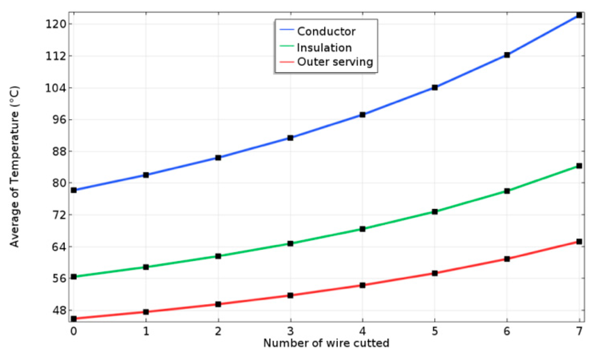
3.5. Effect of Strand Failure on the Thermal Behavior of the Phase

According to the mechanical results of the previous section, we noticed that mechanical stresses were important at the central strand as well as the strands of the first layer, thus, the latter are most likely to fail first. The aim of this stage was to study the effect of the failure of these strands on the thermal behavior of the cable. To proceed, we successively cut the central strand, as well as the strands of the first layer. Figure 12 shows the current density distribution and associated temperature field for four cut wires. We observed a 47% increase in conductor temperature.

Figure 13 shows the evolution of the average temperature of the different components of the cable as a function of the number of wires cut.

4. Conclusions

In this article, we have used FEM to numerically study the influence of damage mechanisms (local plasticity and wire failures) of the submarine power phase conductor on the electrical and thermal behavior of the cable. The models show that with the increase in deformation beyond the yield strength, not only does the mechanical behavior vary, but also the electrical and thermal behavior. Thus, the correlation between mechanical, electrical, and thermal behaviors is clearly emphasized. Multiphysics parameters play key roles simultaneously, in addition to chemical and environmental aspects (e.g., humidity, salt, corrosion-assisted fatigue, etc.) which, in the future, will be the focus of our team. From a technological perspective, this current article can help to ease decision-making with regards to whether the cable (which may show severe defects following handling and shipping-to-deep-sea defects) is performing sufficiently, and therefore can be placed in deep-sea. This can be done, for example, after some damage checking at the end of the manufacturing process and/or after shipping.

As follow-up research, using the thermomechanical fatigue bench developed in our laboratory, these numerical results will be compared with experimental measurements made on the cable to validate the numerical models developed in this article.

References

1. Matine, A.; Bonnard, C.H.; Blavette, A.; Bourguet, S.; Rongere, F.; Kovaltchouk, T.; Schaeffer, E. Optimal Sizing of Submarine Cables from an Electro-Thermal Perspective. In Proceedings of the 12th European Wave and Tidal Energy Conference (EWTEC), Cork, Ireland, 27 August 2017. [Google Scholar]
2. Cheikh, F.E.; Das, R.J.; Drissi-Habti, M.; Ravot, N.; Auzanneau, F. Numerical simulation of high-voltage composite cable for offshore wind. In Proceedings of the 17th European Conference on Composite Materials, ECCM 2016, Munich, Germany, 26–30 June 2016. [Google Scholar]
3. Cheikh, F.E. Modélisations Numérique et Analytique du Comportement Mécanique et Multi-Physique d’une Phase de Câble de Haute-Tension Pour Fermes Offshores. Ph.D. Thesis, Ecole Centrale de Nantes, Nantes, France, 2018. [Google Scholar]
4. Worzyk, T. Submarine Power Cables: Design, Installation, Repair, Environmental Aspects; Springer: Berlin/Heidelberg, Germany, 2009; pp. 51–103. [Google Scholar]
5. Napieralski, P.; Napieralska-Juszczak, E.; Zeroukhi, Y.A. Nonuniform Distribution of Conductivity Resulting from the Stress Exerted on a Stranded Cable During the Manufacturing Process. IEEE Trans. Ind. Appl. 2016, 52, 3886–3892. [Google Scholar] [CrossRef]
6. Liu, D.S.; Chen, D.Y.; Chao, Y.C. A Thermomechanical Study of the Electrical Resistance of Cu Lead Interconnections. J. Electron. Mater. 2006, 35, 958–965. [Google Scholar] [CrossRef]
7. Hruska, F.H. Calculation of stresses in wire rope. Wire Wire Prod. 1951, 26, 766–767. [Google Scholar]
8. Costello, G.A. Theory of Wire Rope, 2nd ed.; Springer: New York, NY, USA, 1997. [Google Scholar]
9. Papailiou, K.O. On the bending stiffness of transmission line conductors. IEEE Trans. Power Deliv. 1997, 12, 1576–1588. [Google Scholar] [CrossRef]
10. Ghoreishi, S.R.; Messager, T.; Cartraud, P.; Davies, P. Validity and limitations of linear analytical models for steel wire strands under axial loading, using a 3D FE model. Int. J. Mech. Sci. 2007, 49, 1251–1261. [Google Scholar] [CrossRef] [Green Version]
11. International Electrotechnical Commission. Electric Cables—Calculation of the Current Rating; IEC 60287-1:2006; IEC: Geneva, Switzerland, 2006. [Google Scholar]
12. M-Bonnet, A. Analyse des Solides Déformables par la Méthode des Eléments Finis; Ecole Polytechnique: Palaiseau, France, 2007. [Google Scholar]
13. Ghoreishi, S. Modelisation Analytique et Caracterisation Experimentale du Comportement de Cables Synthetiques. Master’s Thesis, Ecole Centrale de Nantes, Nantes, France, 2005. [Google Scholar]
14. Jang, J.Y.; Chiu, Y.W. Numerical and experimental thermal analysis for a metallic hollow cylinder subjected to step-wise electro-magnetic induction heating. Appl. Therm. Eng. 2007, 27, 1883–1894. [Google Scholar] [CrossRef]
15. Long, C. Essential Heat Transfer, 1st ed.; Prentice Hall: Upper Saddle River, NJ, USA, 1999. [Google Scholar]
16. Churchill, S.; Chu, H. Correlating equations for laminar and turbulent free convection rom a horizontal cylinder. Int. J. Heat Mass Transf. 1975, 18, 1049–1053. [Google Scholar] [CrossRef]
Figure 1. Elasto-plastic behavior of a metallic material.
Energies 12 01009 g001
Figure 2. Structure of the cable phase (left); the photograph (right). Source: NEXANS.
Energies 12 01009 g002
Figure 3. Multilayer conductor (1 + 6 + 12).
Energies 12 01009 g003
Figure 4. Evolution of electrical conductivity as a function of mechanical stresses experimentally obtained for a copper wire [5].
Energies 12 01009 g004
Figure 5. (a) Finite element mesh, and (b) simulated stress–strain curve.
Energies 12 01009 g005
Figure 6. Distribution of the von Mises stress in the cable in MPa (right in elastic range; left in plastic range).
Energies 12 01009 g006
Figure 7. Distribution of the von Mises stress in the conductor in MPa in the plastic range (left) and its correspondence in electrical conductivity (right).
Energies 12 01009 g007
Figure 8. Evolution of the axial stress as a function of the electrical resistance in (µΩ) the conductor.
Energies 12 01009 g008
Figure 9. Distribution of the temperature field in °C (right) and the magnetic field in T (left) in equilibrium.
Energies 12 01009 g009
Figure 10. Distribution of the temperature field in °C when the conductor is mechanically damaged (left 140%; right 168%).
Energies 12 01009 g010
Figure 11. Average temperature in the cable as a function of the plasticity level.
Energies 12 01009 g011
Figure 12. Distribution of the temperature field in °C (right) and current density in A/m² (left) when the conductor is mechanically damaged (six-wire failure).
Energies 12 01009 g012
Figure 13. Average temperature in the cable as a function of number of cut wires.
Energies 12 01009 g013