Effect of Different Interval Lengths in a Rolling Horizon MILP Unit Commitment with Non-Linear Control Model for a Small Energy System

Abstract

In this paper, a fixed electricity producer park of both a short- and long-term renewable energy storage (e.g., battery, power to gas to power) and a conventional power plant is combined with an increasing amount of installed volatile renewable power. For the sake of simplicity, the grid is designed as a single copper plate with island restrictions and constant demand of 1000 MW; the volatile input is deducted from scaled 15-min input data of German grid operators. A mixed integer linear programming model is implemented to generate an optimised unit commitment (UCO) for various scenarios and configurations using CPLEX^® as the problem solver. The resulting unit commitment is input into a non-linear control model (NLC), which tries to match the plan of the UCO as closely as possible. Using the approach of a rolling horizon the result of the NLC is fed back to the interval of the next optimisation run. The problem’s objective is set to minimise CO₂ emissions of the whole electricity producer park. Different interval lengths are tested with perfect foresight. The results gained with different interval lengths are compared to each other and to a simple heuristic approach. As non-linear control model a characteristic line model is used. The results show that the influence of the interval length is rather small, which leads to the conclusion that realistic forecast lengths of two days can be used to achieve not only a sufficient quality of solutions, but shorter computational times as well.

1. Introduction

The expansion of volatile renewable energy (VRE) is a major project, that many countries decided to undergo as part of their commitments under the UN Paris Climate Change Conference of 2016 [1]. Various energy system configurations (i.e., distribution of technologies, their installed rated power and capacities) are suggested to meet the goals of e.g., the German Energiewende [2]. Energy systems can consist of VRE plants (e.g., wind, photovoltaic, concentrating solar power), of renewable storage facilities (e.g., batteries, power to gas to power, pumped hydro) and of conventional storage facilities or “primary energy storages” [3] (e.g., combined cycle gas turbine (CCGT), coal-fired steam power plant). To avoid confusion, in this paper the term “energy storage” is used solely for renewable storage facilities or “secondary energy storages” [3]. “Primary energy storages” are referred to as conventional power plants throughout this paper.

For this work a small energy system without transmission losses (often referred to as “copper plate”) and no possible external source or sink of power (often referred to as “island restriction”), in the following referred to as “copper plate island”, is the test system. The copper plate island consists of a CCGT power plant, a short-term and a long-term energy storage and varying instalments of solar and wind power. Installed solar and wind power are equally distributed across all configurations and their installed power is given as VRE power in MW_each, meaning the installed power each generation type has in a given configuration. As demand for the energy system, a constant power of 1000 MW is defined.

To utilise given energy system configurations to their maximum potential as well as test their feasibility, time series simulation is a commonly used tool. These simulations need some kind of unit commitment (UC) for dispatching the plants in the given energy system.

The methods for UC can vary from heuristic to non-linear optimisation problems, from deterministic to stochastic with all their methodical benefits and drawbacks [4,5]. A popular approach is the formulation of the energy system as a mixed integer linear problem (MILP) for small [6] to larger systems [7,8]. Most often the optimisation problem is formulated to find the best solution for the entire time series (e.g., one year) at once, which can become very complex and time consuming and might make local computing resources incompatible [9]. To solve this problem, the use of a rolling horizon became more and more popular in recent years [5,10,11,12].

In [13] a comprehensive review of energy system modelling tools can be found. Seventy-five models were categorised in purpose, approach, methodology, temporal resolution, modelling horizon, spatial resolution and coverage and availability. These models were then discussed and their features listed. More than half of the presented models use a linear programming or MILP approach. The use of rolling horizons is however rarely mentioned.

Recently developed frameworks such as the one of [11] demonstrate the significance of the rolling horizon approach. This framework was developed to show the effect of different interval lengths (e.g., five hours or four days) on a one-day unit commitment problem. It would allow for modification of the MILP results in order to adjust for uncertainties or new information, but was not used in [10]. The framework was updated in [14] to model start-up times and tested for different rolling horizon interval lengths between two and 24 h. [15] presented a different framework, where the rolling horizon was implemented for a similar reason, but added an optional economic dispatch algorithm to adjust the suggested UC. This is to model market behaviour more properly.

This use of cascading UC to mimic the behaviour of a day-ahead and intra-day market was implemented by [16]. The market behaviour was modelled by a 24 h MILP unit commitment with a stochastically generated VRE forecast for the day ahead and a 4 h non-linear point algorithm to minimise the cost associated with diverging from the day-ahead UC.

A similar approach of stochastic programming for the UC was investigated and tested against a deterministic approach by [17]. The stochastic problem was tested in various configurations of rolling horizon lengths for the problem and solution aggregation on a larger energy system with electric grid constraints. In a similar fashion this research topic was investigated by [18], with the difference that in [18] various lengths for the final unit commitment—minimising the divergence from the stochastic forecast—were tested. Another difference lies in the configuration of the underlying energy system, whereby both [17,18] use different kinds of short-term energy storage devices and no long-term energy storage devices.

Investigation of lengths for the rolling horizon was done by [19] to find the optimal use of power plant flexibility considering the start-up and maintenance related problems of CCGT power plants.

Focusing on a thermal energy storage device for the medium term, [20] investigated a rolling horizon with a week-long forecast against a previous research with a day-ahead forecast and found the results to be better for the week-long unit commitment.

To adjust for non-linear behaviour of the system [20,21] did a piecewise linearisation of the price-effects that influenced the objective function. The focus of [21] was the usage of upper-, lower-bound or mean value of the linearised piece from the price function.

This paper focusses on energy system feasibility for future energy systems, for which [22] reviewed various energy system simulation models. The difference to the previously discussed systems is that future energy systems contain long-term energy storage devices. In this case, the UC might need longer forecasting lengths, as their name implies. It should be noted however, that [16,20,21] still adjust their models for non-linearities despite their rather short interval length.

For a better integration of long-term storages [23] integrates the rolling horizon approach to apply different levels of detail. For the exact UC, a complex model is used with short horizons, which is thought to not encompass the characteristics of long-term storages. A less complex model is used for the entire time frame, to set the characteristics for the exact planning.

Similarly [24] applied the use of a less complex model, but for a whole year simulation. The research investigated the use of an evolutionary algorithm for the energy system configuration with an underlying two level MILP UC. For the lower level a one-day rolling horizon MILP UC was implemented. The parameters of the MILP were generated from a non-linear model. Unfortunately the model of [24] does not ensure, that the long-term storage is filled to its initial state of charge (SOC) at the end of the simulation.

The rolling horizon is done here primarily to save simulation time, as [25] proposed, where the effect of different lengths of the rolling horizon and their effect on simulation time und quality of the solution was investigated. The quality of the solution was judged against the solution of a MILP UC solution for the entire time frame at once.

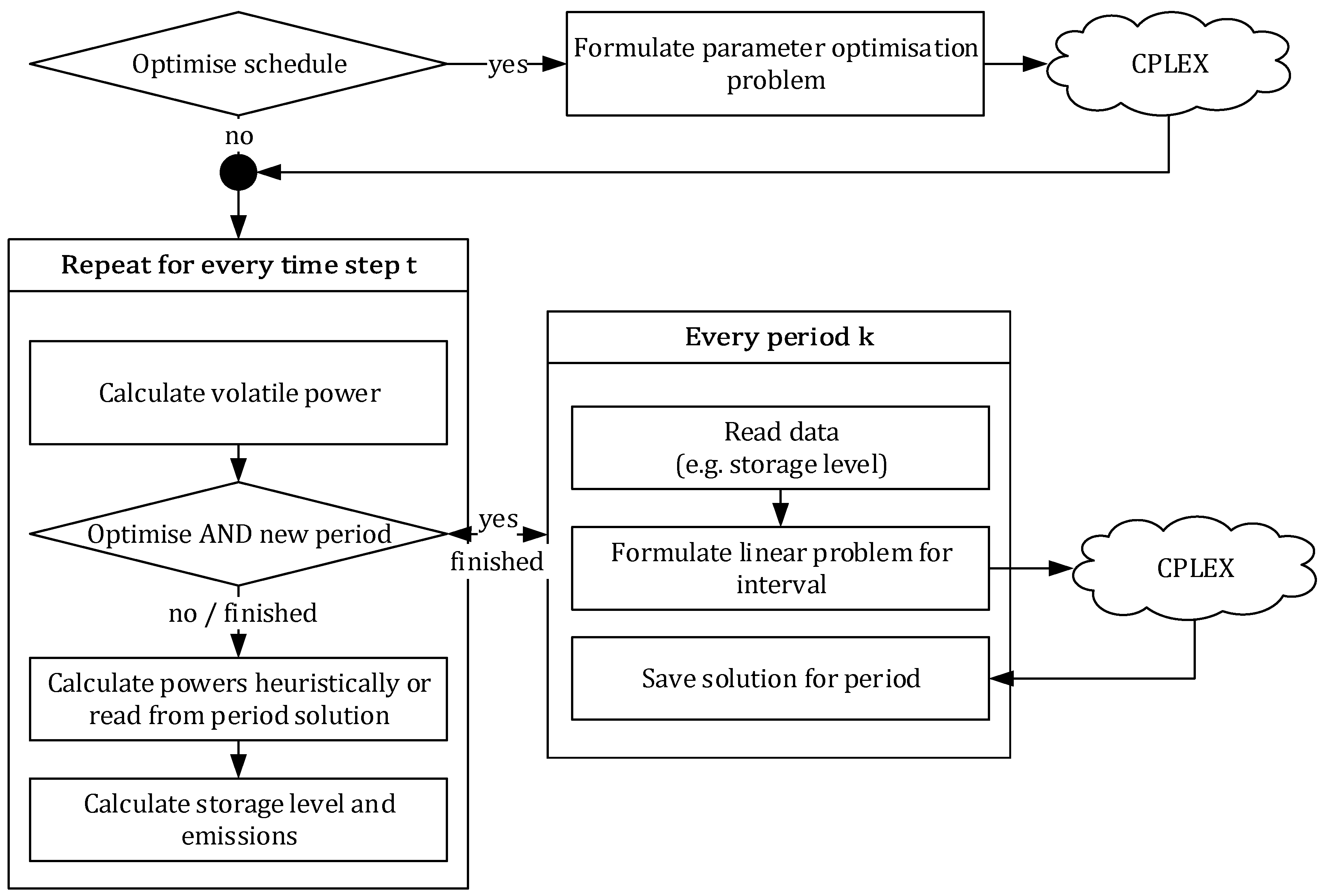
This paper introduces a different modelling approach for the solution of UC problems, in which the solution of a MILP UC is handed to a non-linear control model (NLC). That way the feasibility of the proposed UC can be tested. Further the MILP formulation uses the approach of [26] to model part-load behaviour more correctly, where the parameters of the MILP and initial values in a rolling horizon operation are generated from the NLC. With this approach, the effect of the interval length (see Section 2.1) in a rolling horizon problem becomes the research focus of this paper. To our knowledge, this has not been addressed with an NLC before.

To determine the effect of the interval lengths the results of MILP unit commitment optimisations (UCO) with varying temporal settings are compared to a unit commitment with a heuristic approach (UCH). The CO₂ emissions of the electricity producer park are the minimisation objective of the MILP, which is why the specific CO₂ emissions of the electricity producer park are used as the primary quality measure of the UC results. Additionally, the share of storages, meaning the amount of energy delivered by the energy storage devices in respect to total demand, acts as an indicator of difference between UCO and UCH.

A characteristic line model, namely CharL (see Supplementary Materials), is inherent to the UCH and used as an NLC for the UCO, instead of simply aggregating the MILP results (see Section 2.1).

2. Model Structure and Materials

In this work, the used model’s base functionality is a model of characteristic lines, such as the efficiency curve of a thermal power plant. Figure 1 exemplarily shows characteristic lines of the relative efficiency over the relative power for combined and open cycle gas turbines according to [27]. For application in the model, those curves are scaled with net efficiencies and used to compute the use of fuel and emissions of CO₂ at any given point of time in the simulation.

2.1. Program Flow of CharL

The CharL library can be used to calculate time series of given energy system configurations. It is possible to simulate on a UCH or by incorporation of a UCO generated operation plan as the simplified program flow in Figure 2 shows. The displayed scheme starts after the initial data reading and initialisation and begins with assessing whether the unit commitment is done heuristically or via MILP optimisation. In the latter case necessary parameters for the MILP model (see Section 2.6.3) are optimised. Both paths then start the modelling process for all time steps $t$. Every time step starts with the assessment of VRE power. If the time step is at the start of a new optimisation period and the unit commitment is not done heuristically, a MILP is formulated after reading the VRE power forecast for the current interval and technological constraints (e.g., storage level) from the previous time step. Afterwards the MILP is handed to the commercial solver CPLEX [28], whose final solution is saved (see Figure 2) for all timesteps of the period k (see Figure 3). After the optimisation is finished or when the unit commitment is done heuristically, the program continues at the time step $t$ and operates first the storage units and then the conventional power plant units as close as possible to the proposed unit commitment. The proposed unit commitment is followed for next timesteps until the beginning of a new period starts, where a new MILP is formulated and solved. The level for the storage units and the emissions are calculated after the proposed powers of the respective units were deemed valid. The results are evaluated after finishing the last time step. The program is held entirely in C++ with the external libraries FLOPC++ [29] and OSI for the formulation of the MILP and the Qt library solely for the GUI (see Supplementary Materials).

As previously stated, the formalisation of the linear problem is repeated at every new beginning of a period but formulated for the length of an interval. The term “interval” hereby refers to the time period that the UCO problem is formulated for, while the term “period” means the time period for which the result of the UCO is saved and input into the NLC. The interval length therefore is always equal or greater than the period length. Greater interval lengths lead to an overhang that is (re-)solved in the following period(s). The overhang prevents consecutive operation plans from being independent of each other. This process can be seen in Figure 3 and is called a rolling horizon.

2.2. Renewable Energy Modelling

For complexity and computational resources the renewable energy profile was modelled using scaled solar and wind production of 2015 as made publicly available by the German transmission system operators (TSO) [30,31,32,33,34,35,36,37]. The scaling was done using the monthly installed capacities of solar and wind, which are provided by the TSOs [38]. The resulting production profiles for wind and solar of 2015 can be seen in Figure 4. Lastly, for the greater interval length and therefore bigger optimisation problems, these curves are averaged to result in hourly temporal resolution.

2.3. Modelling Residual Power Generators

The residual power generators are the (renewable) energy storage devices’ discharge units and the conventional power plants, which could be considered a discharge unit of a conventional energy storage device (see Section 1). This results in a similar modelling approach, namely using the efficiency curve to calculate the needed power of the input form of energy.

Since energy storage devices can only discharge, if there is energy already stored (i.e., after a charging process), the charging process has to be modelled using a second efficiency curve. Additionally, the energy storage devices have a self-discharge rate when not in use, as [39] defined self-discharge only under open-circuit conditions. Accordingly, a fixed round-trip efficiency, meaning the efficiency of power to storage to power, is not used in this work.

Furthermore, maximum load gradients are considered for all units. The emissions of power plants are calculated using their fuel’s respective specific emission per MWh_th as an additional parameter. The NLC considers start-up times as the corresponding functions are implemented. For this paper, the residual power generators are parameterised so that the start-up times have no influence on the UC. That way the MILP model (see Section 2.5) can resemble the NLC more closely.

2.4. Heuristic Unit Commitment

The UCH follows a very simple approach to integrate any excess energy of VRE plants into energy storage devices and meet any resulting residual load from the energy storage devices, if possible. Any further resulting residual load will be matched by the conventional thermal power plants.

The UCH iteratively solves the entire time series until the storage levels of all storages at the initial and final timestep do not change any further from one run to the next within a tolerance of 1 MWh.

2.5. MILP Formulation

The MILP formulation is designed to mirror the modelling approach of CharL as close as possible. The following equations are written as they are programmed using the FLOPC++-library [29] to address the solver CPLEX [28]. Using Gurobi [40] as the solver would have been possible as well, but was disregarded due to practical reasons.

2.5.1. Constraints to Model Thermal Power Plants

Thermal power plants are modelled with a semi-continuous operating range. A binary variable $\psi$ states, whether the unit is online or offline, while $P_{\min }$ and $P_{\max }$ are minimum and maximum limits for the power generation $P$, which is fed into the grid. For every period $k\in K$ the constraints need to be formulated for all generating plants $g\in G$ and time steps $t\in T_k$:

$$\begin{gathered} P\left(g,t\right)\ge P_{\min }\left(g\right)\cdot \psi \left(g,t\right);\hspace{1em}\forall g\in G\hspace{1em}\forall t\in T_k. \\ P\left(g,t\right)\le P_{\max }\left(g\right)\cdot \psi \left(g,t\right);\hspace{1em}\forall g\in G\hspace{1em}\forall t\in T_k. \end{gathered}$$

(1)

In addition to the operating range of the units, ramping limits $R$ are applied using the following equations considering the length of a time step $\tau$. It is possible to differentiate between the maximum upward and downward gradient:

$$\begin{gathered} P\left(g,t-1\right)-P\left(g,t\right)\le R_{\mathrm{down}}\left(g\right)\cdot \tau ;\hspace{1em}\forall g\in G\hspace{1em}\forall t\in T_k. \\ P\left(g,t-1\right)-P\left(g,t\right)\ge -R_{\mathrm{up}}\left(g\right)\cdot \tau ;\hspace{1em}\forall g\in G\hspace{1em}\forall t\in T_k. \end{gathered}$$

(2)

For $t=T_{k,0}$ the variable for $t-1$ is replaced by data from the non-linear control of the previous period.

The efficiency of a power generation unit usually shows non-linear characteristics, which cannot be integrated directly into a MILP formulation. In accordance with [26], the efficiency characteristic is implemented using the load-unspecific basic demand. Hereby, the power on the unit side (and therefore the fuel demand) is described with $P_{\mathrm{u}}$:

$$P\left(g,t\right)=a\left(g\right)\cdot P_{\mathrm{u}}\left(g,t\right)-a\left(g\right)\cdot b\left(g\right)\cdot P_{\mathrm{nom}}\left(g\right)\cdot \psi \left(g,t\right);\hspace{1em}\forall g\in G\hspace{1em}\forall t\in T_k.$$

(3)

Hereby a constant loss factor or basic demand, which is calculated in relation to the nominal power of the plant $P_{\mathrm{nom}}$, is subtracted in addition to using a constant load-unspecific efficiency $a$. The parameterisation of $a$ and $b$ allows for modelling the non-linear efficiency characteristic with sufficient accuracy (see Section 2.6.3). In comparison to a piecewise linearisation, less variables and especially no additional binary variables ought to be used, which leads to lower computational effort [41].

2.5.2. Constraints to Model Energy Storage Devices

For units of the generic storage class $s\in S$, power and ramping limits are formulated according to Section 2.5.1. It is distinguished between the operating conditions “charging” and “discharging”:

$$\begin{gathered} P_{\mathrm{ch}}\left(s,t\right)\ge P_{\mathrm{ch},\min }\left(s\right)\cdot {\psi }_{\mathrm{ch}}\left(s,t\right);\hspace{1em}\forall s\in S\hspace{1em}\forall t\in T_k. \\ {P}_{\mathrm{charge}}\left(s,t\right)\le P_{\mathrm{ch},\max }\left(s\right)\cdot {\psi }_{\mathrm{charge}}\left(s,t\right);\hspace{1em}\forall s\in S\hspace{1em}\forall t\in T_k. \\ {P}_{\mathrm{discharge}}\left(s,t\right)\ge P_{\mathrm{dis},\min }\left(s\right)\cdot {\psi }_{\mathrm{dis}}\left(s,t\right);\hspace{1em}\forall s\in S\hspace{1em}\forall t\in T_k. \\ {P}_{\mathrm{discharge}}\left(s,t\right)\le P_{\mathrm{dis},\max }\left(s\right)\cdot {\psi }_{\mathrm{dis}}\left(s,t\right);\hspace{1em}\forall s\in S\hspace{1em}\forall t\in T_k. \end{gathered}$$

(4)

$$\begin{gathered} P_{\mathrm{ch}}\left(s,t-1\right)-P_{\mathrm{ch}}\left(s,t\right)\le R_{\mathrm{ch},\mathrm{down}}\left(s\right);\hspace{1em}\forall s\in S\hspace{1em}\forall t\in T_k. \\ {P}_{\mathrm{ch}}\left(s,t-1\right)-P_{\mathrm{ch}}\left(s,t\right)\ge -R_{\mathrm{ch},\mathrm{up}}\left(s\right);\hspace{1em}\forall s\in S\hspace{1em}\forall t\in T_k. \\ {P}_{\mathrm{dis}}\left(s,t-1\right)-P_{\mathrm{dis}}\left(s,t\right)\le R_{\mathrm{dis},\mathrm{down}}\left(s\right);\hspace{1em}\forall s\in S\hspace{1em}\forall t\in T_k. \\ {P}_{\mathrm{dis}}\left(s,t-1\right)-P_{\mathrm{dis}}\left(s,t\right)\ge -R_{\mathrm{dis},\mathrm{up}}\left(s\right);\hspace{1em}\forall s\in S\hspace{1em}\forall t\in T_k. \end{gathered}$$

(5)

For $t=T_{k,0}$ the variable for $t-1$ is replaced by data from the non-linear control of the previous period. Because the operating conditions are exclusive, simultaneous charging and discharging of the storage is inhibited by Equation (6):

$${\psi }_{\mathrm{ch}}\left(s,t\right)+{\psi }_{\mathrm{dis}}\left(s,t\right)\le 1;\hspace{1em}\forall s\in S\hspace{1em}\forall t\in T_k.$$

(6)

The efficiency characteristics for both operating conditions are modelled also using the load-unspecific basic demand as described in Section 2.5.1 (see Equation (5)):

$$\begin{gathered} P_{\mathrm{ch},\mathrm{u}}\left(s,t\right)=a_{\mathrm{ch}}\left(s\right)\cdot P_{\mathrm{ch}}\left(s,t\right)-a_{\mathrm{ch}}\left(s\right)\cdot b_{\mathrm{ch}}\left(s\right)\cdot P_{\mathrm{ch},\mathrm{nom}}\left(s\right)\cdot {\psi }_{\mathrm{ch}}\left(s,t\right); \\ \forall s\in S\hspace{1em}\forall t\in T_k. \\ {P}_{\mathrm{dis},\mathrm{u}}\left(s,t\right)=a_{\mathrm{dis}}\left(s\right)\cdot P_{\mathrm{dis}}\left(s,t\right)-a_{\mathrm{dis}}\left(s\right)\cdot b_{\mathrm{dis}}\left(s\right)\cdot P_{\mathrm{dis},\mathrm{nom}}\left(s\right)\cdot {\psi }_{\mathrm{dis}}\left(s,t\right); \\ \forall s\in S\hspace{1em}\forall t\in T_k. \end{gathered}$$

(7)

To apply the efficiency losses for a storage unit, a distinction is made between the power on the grid side $P_{\mathrm{ch}}$ and the power as seen by the storage $P_{\mathrm{ch},\mathrm{u}}$.

Since Equation (7) yields the possibility for no power on the storage but power on the grid side, which in return is beneficial for the objective function (14), the following two equations are necessary and state that the efficiency of each operating mode ought to be always below one:

$$\begin{gathered} P_{\mathrm{ch},\mathrm{u}}\left(s,t\right)\le P_{\mathrm{ch}}\left(s,t\right);\hspace{1em}\forall s\in S\hspace{1em}\forall t\in T_k. \\ {P}_{\mathrm{dis},\mathrm{u}}\left(s,t\right)\ge P_{\mathrm{dis}}\left(s,t\right);\hspace{1em}\forall s\in S\hspace{1em}\forall t\in T_k. \end{gathered}$$

(8)

The model only considers the net capacity of a storage $C_{\mathrm{net}}$. The upper and lower bounds for the storage level $E$ can therefore be set as follows:

$$\begin{gathered} \underset{\_}{E}\left(s,t\right)=0;\forall s\in S\forall t\in T_k. \\ \overline{E}\left(s,t\right)=C_{\mathrm{net}}\left(s\right);\forall s\in S\forall t\in T_k. \end{gathered}$$

(9)

The storage level of an energy storage device is calculated based on the storage level of the previous time step, the self-discharge rate $\xi$ and the charging/discharging power on the storage side $P_{\mathrm{ch},\mathrm{u}}$ and $P_{\mathrm{dis},\mathrm{u}}$, respectively, in the current time step:

$$\begin{gathered} E\left(s,t\right)=E\left(s,t-1\right)\cdot \left[1-\xi \left(s\right)\cdot \tau \right]+\tau \cdot \left[P_{\mathrm{ch},\mathrm{u}}\left(s,t\right)-P_{\mathrm{dis},\mathrm{u}}\left(s,t\right)\right]; \\ \forall s\in S\forall t\in T_k. \end{gathered}$$

(10)

For $t=T_{k,0}$ the variable for $t-1$ is replaced by data from the non-linear control of the previous period. To ensure a closed energy balance over the whole simulation time frame, boundary conditions need to guarantee the equality of the initial storage level in the first interval of the simulation and the final storage level of the last interval. One problem regarding the rolling horizon approach is the missing communication between the first and the last loop as to what initial, and therefore final, storage level might be suboptimal.

To surpass that problem, the initial storage level $E_{\mathrm{init}}$ is passed to the model as data point. The value for each storage unit is received via the UCH approach described in Section 2.4. The following constraints ensure a closed energy balance for each storage within a tolerance of one percent net capacity:

$$E\left(s,0\right)=E_{\mathrm{init}}\left(s\right);\forall s\in S;\mathrm{if}\mathrm{first}\mathrm{period}$$

(11)

and:

$$\begin{array}{c}\underset{\_}{E}\left(s,t_{\mathrm{period}}\right)=E_{\mathrm{init}}\left(s\right)\pm 0.01\cdot C_{\mathrm{net}}\left(s\right);\forall s\in S\\ \overline{E}\left(s,t_{\mathrm{period}}\right)=E_{\mathrm{init}}\left(s\right)\pm 0.01\cdot C_{\mathrm{net}}\left(s\right);\forall s\in S\end{array}\}\mathrm{if}{t}_{\mathrm{period}}=T_{\mathrm{total}}$$

(12)

2.5.3. Constraints to Model the Energy System

The electric demand $P_{\mathrm{demand}}$ and the renewable power generation $P_{\mathrm{volatile}}$ are given as input data for the system balance, which is formulated in Equation (13), to match demand and generation in the grid for each time step:

$$\begin{gathered} P_{\mathrm{demand}}\left(t\right)=P_{\mathrm{volatile}}\left(t\right)+{\displaystyle \sum }^{\mathrm{G}}P\left(g,t\right)-{\displaystyle \sum }^{\mathrm{S}}{P}_{\mathrm{ch}}\left(s,t\right) \\ +{\displaystyle \sum }^{\mathrm{S}}{P}_{\mathrm{dis}}\left(s,t\right)+P_{{\mathrm{slack}}_{+}}\left(t\right)-P_{{\mathrm{slack}}_{-}}\left(t\right);\hspace{1em}\forall t\in T_k. \end{gathered}$$

(13)

Slack variables $P_{\mathrm{slack}}$ for a positive and negative deviation of load and generation are established to ensure solvability of the optimisation problem.

2.5.4. Objective Function

As a model of the electricity market is not yet integrated in the optimisation problem, the objective function (14) is set to minimise the emissions throughout the regarding time frame:

$$\begin{gathered} \underset{}{\min }\left\{{\displaystyle \sum }^T\tau \cdot \left[{\displaystyle \sum }^{\mathrm{G}}{P}_{\mathrm{u}}\left(g,t\right)\cdot e\left(g\right)-{\displaystyle \sum }^{\mathrm{S}}{P}_{\mathrm{ch},\mathrm{u}}\left(s,t\right)\cdot e_{\mathrm{stor}}+{\displaystyle \sum }^{\mathrm{S}}{P}_{\mathrm{dis},\mathrm{u}}\left(s,t\right)\cdot e_{\mathrm{stor}} \\ +P_{{\mathrm{slack}}_{+}}\left(t\right)\cdot e_{{\mathrm{pen}}_{+}}+P_{{\mathrm{slack}}_{-}}\left(t\right)\cdot e_{{\mathrm{pen}}_{-}}\right]\right\} \end{gathered}$$

(14)

The usage of the slack variables should be avoided to achieve equality of demand and supply. However, in time steps where storages are full and there is high renewable generation, those slack variables are needed to find valid solutions. Therefore, the specific emissions for the slack variables $e_{\mathrm{pen}}$ are set to high values as a penalty, so that those variables are only contributing to the solution when no other can be found.

The penalty for power surpluses serves two functions in that it not only serves the solution process, but also incentivises the use of storage devices. This becomes necessary when the excess of energy cannot be used within the current interval. The virtual storage emissions are set to incentivise the usage of more efficient storages. When not in place an overuse of the less efficient long-term storage was observed as the long-term storage device may reduce conventional and penalty usage by the same amount as the short-term storage within a single interval.

2.6. Temporal and Technical Scenario Configuration

Throughout this paper, a scenario is defined as a set of period and interval length and configuration is defined as the installed powers, capacities and set of units. Due to the complexity of the constraints and the high temporal resolution of the data, a copper plate island with a rather small number of actors is chosen. This makes the result not applicable to larger systems, which is acceptable for this paper, since the effect of different interval lengths in UCO is the main research target of this paper rather than an accurate representation of a real energy system.

The interval lengths were chosen to represent possible ranges from forecast lengths of high resolution, local weather models [42], like the two and three days intervals, up to forecast lengths of low resolution, global weather models [43] with the 5 and 14 days intervals. The 30 days interval was set to test whether there is need for even longer forecast lengths and the 365 days interval was set as it is commonly used in UC models [6,7,8,41,44]. To achieve or rather allow a similar computation time the MILP-solver settings have to be adjusted for the varying interval lengths. Those settings can be seen in

Table 1. Temporal configurations of the scenarios and abort criteria for MILP.

Scenario	Hardware Used	Interval Length	Period Length	Abort Criteria
	(see Table A1)			Max. Time in s	Rel. Gap
a	PC 1	2 days	1 day	1200	1.0 × 10−6
b	PC 2	3 days	1 day	2400	1.0 × 10−6
c	PC 3	5 days	2 days	3600	1.0 × 10−5
d	PC 4	14 days	5 days	10,800	1.0 × 10−5
e	PC 3	30 days	10 days	21,600	1.5 × 10−5
f	PC 1	365 days	365 days	100,000	1.0 × 10−4

, where interval and period lengths are given as time in days.

For the 365 days scenario the maximum time abort criteria was set comparatively low, since the program tended to crash otherwise.

Abort criteria for the MILP solver to stop its solution process can be found in Table 1 as well. Abort criteria are the time for the solution process and the relative gap. The values were chosen to limit the overall solution time to a similar value, but do not necessarily lead to equal overall solution times (see

Table A5. Statistics for 2 days optimisation of MILP solver.

Installed Power Each Wind and Solar in MW	Statistics of Rolling Horizon Regarding the Time of the Solution		Statistics of Rolling Horizon Regarding the Relative Gap of the Solutions All in -
	Average Time in s	# of Times Time Limit Reached	Min.	Max.	Average	Standard Deviation	# of Times No Solution Found
1000	255.22	68	0	2.81 × 10−5	8.30 × 10−5	7.54 × 10−4	0
1250	296.50	81	0	7.53 × 10−5	3.35 × 10−4	4.14 × 10−3	0
1500	232.86	61	0	6.01 × 10−5	2.28 × 10−4	2.74 × 10−3	0
1750	249.27	65	0	1.13 × 10−4	7.34 × 10−4	1.26 × 10−2	0
2000	298.44	80	0	2.08 × 10−4	1.47 × 10−3	2.61 × 10−2	1
2250	350.70	96	0	1.36 × 10−4	6.60 × 10−4	1.00 × 10−2	0
2500	373.67	102	0	2.79 × 10−4	1.56 × 10−3	2.25 × 10−2	0
2750	331.37	91	0	1.39 × 10−4	4.88 × 10−4	4.60 × 10−3	4
3000	357.32	98	0	3.48 × 10−4	3.67 × 10−3	6.99 × 10−2	4
3250	361.49	99	−4.00 × 10−6	3.47 × 10−4	1.65 × 10−3	2.23 × 10−2	4
3500	306.08	79	0	5.56 × 10−4	3.56 × 10−3	4.40 × 10−2	2
3750	303.41	83	−3.31 × 10−3	4.83 × 10−4	2.32 × 10−3	2.76 × 10−2	2
4000	372.83	103	0	4.84 × 10−4	1.52 × 10−3	1.21 × 10−2	2
4250	385.11	109	−5.83 × 10−4	7.64 × 10−4	3.08 × 10−3	4.95 × 10−2	1
4500	416.41	116	−1.78 × 10−4	7.68 × 10−4	2.41 × 10−3	1.99 × 10−2	3
4750	396.97	114	0	8.16 × 10−4	3.28 × 10−3	4.81 × 10−2	1
5000	474.40	135	0	1.06 × 10−3	3.79 × 10−3	5.75 × 10−2	1

,

Table A6. Statistics for 3 days optimisation of MILP solver.

Installed Power Each Wind and Solar in MW	Statistics of Rolling Horizon Regarding the Time of the Solution		Statistics of Rolling Horizon Regarding the Relative Gap of the Solutions all in -
	Average Time in s	# of Times Time Limit Reached	Min.	Max.	Average	Standard Deviation	# of Times No Solution Found
1000	625.84	89	0	2.07 × 10−5	5.58 × 10−5	5.55 × 10−4	0
1500	696.96	101	0	5.91 × 10−5	2.19 × 10−4	3.03 × 10−3	0
2000	936.51	138	0	1.79 × 10−4	1.16 × 10−3	2.07 × 10−2	0
2500	1125.33	158	0	2.78 × 10−4	1.97 × 10−3	3.29 × 10−2	0
3000	1064.41	151	−1.00 × 10−6	2.55 × 10−4	1.58 × 10−3	2.91 × 10−2	1
3500	900.47	125	0	1.01 × 10−3	7.11 × 10−3	8.81 × 10−2	2
4000	931.97	131	0	7.44 × 10−4	3.31 × 10−3	5.32 × 10−2	1
4500	1126.80	165	0	1.18 × 10−3	3.60 × 10−3	3.54 × 10−2	0
5000	1136.87	164	−2.73 × 10−3	1.63 × 10−3	5.42 × 10−3	4.91 × 10−2	4

,

Table A7. Statistics for 5 days optimisation of MILP solver.

Installed Power Each Wind and Solar in MW	Statistics of Rolling Horizon Regarding the Time of the Solution		Statistics of Rolling Horizon Regarding the Relative Gap of the Solutions All in -
	Average Time in s	# of Times Time Limit Reached	Min.	Max.	Average	Standard Deviation	# of Times No Solution Found
1000	1105.31	104	1.00 × 10−6	2.37 × 10−5	3.78 × 10−5	2.55 × 10−4	0
2000	2217.89	107.5	0	1.41 × 10−4	3.98 × 10−4	2.87 × 10−3	0
3000	2445.49	120.5	0	2.03 × 10−4	4.67 × 10−4	5.54 × 10−3	0
4000	2205.14	106.5	0	9.62 × 10−4	2.82 × 10−3	2.26 × 10−2	0
5000	2229.26	109.5	0	1.26 × 10−3	3.21 × 10−3	2.66 × 10−2	0

,

Table A8. Statistics for 14 days optimisation of MILP solver.

Installed Power Each Wind and Solar in MW	Statistics of Rolling Horizon Regarding the Time of the Solution		Statistics of Rolling Horizon Regarding the Relative Gap of the Solutions All in -
	Average Time in s	# of Times Time Limit Reached	Min.	Max.	Average	Standard Deviation	# of Times No Solution Found
1000	1975.74	13	7.00 × 10−6	3.16 × 10−5	5.46 × 10−5	2.41 × 10−4	0
2000	6005.35	38	1.00 × 10−5	1.16 × 10−4	2.14 × 10−4	1.51 × 10−3	0
3000	6487.44	43	0	2.51 × 10−4	3.97 × 10−4	2.29 × 10−3	0
4000	3013.66	18	0	7.99 × 10−4	2.80 × 10−3	2.00 × 10−2	0
5000	3940.38	25	−1.30 × 10−5	2.40 × 10−3	6.98 × 10−3	4.33 × 10−2	0

,

Table A9. Statistics for 30 days optimisation of MILP solver.

Installed Power Each Wind and Solar in MW	Statistics of Rolling Horizon Regarding the Time of the Solution		Statistics of Rolling Horizon Regarding The Relative Gap of the Solutions All in -
	Average Time in s	# of Times Time Limit Reached	Min.	Max.	Average	Standard Deviation	# of Times No Solution Found
1000	11,190.58	16.5	1.30 × 10−5	5.79 × 10−5	7.75 × 10−5	3.42 × 10−4	0
2000	21,609.54	36.5	4.50 × 10−5	2.08 × 10−4	1.54 × 10−4	6.99 × 10−4	0
3000	20,163.36	34	1.50 × 10−5	7.14 × 10−4	6.50 × 10−4	2.52 × 10−3	0
4000	7155.09	12	0	2.77 × 10−4	6.53 × 10−4	3.39 × 10−3	0
5000	9712.99	15.5	0	2.56 × 10−3	9.59 × 10−3	5.88 × 10−2	0

and

Table A10. Statistics for 365 days optimisation of MILP solver.

Installed Power Each Wind and Solar in MW	Statistics of Rolling Horizon Regarding the Time of the Solution		Statistics of Rolling Horizon Regarding the Relative Gap of the Solutions All in -
	Average Time in s	# of Times Time Limit Reached	Relative Gap	Standard Deviation	# of Times No Solution Found
1000	100,036.54	1	1.77 × 10−4	0	0
2000	100,047.74	1	4.43 × 10−4	0	0
3000	100,076.56	1	1.04 × 10−3	0	0
4000	100,092.65	1	3.19 × 10−2	0	0
5000	100,053.86	1	6.59 × 10−3	0	0

). Other than that, the default settings of FLOP++ and CPLEX for a branch-and-bound solution were used.

2.6.1. The Actors

For the sake of simplicity and reproducibility, a constant demand of 1000 MW all throughout the year was chosen. This is deemed acceptable for the research target at hand as the UC problem resulting from the VRE generation is seen as sufficiently complex. As conventional power plant, using the primary storage natural gas, a combined cycle gas turbine (CCGT) power plant was chosen with a rated power output of 1000 MW, so that it is always able to cover any remaining residual load. As a short-term energy storage device, a battery with 5000 MWh_net is chosen. A long-term energy storage device consists of an electrolyser for conversion of power to hydrogen and its own CCGT plant for reconversion of hydrogen to power. As storage capacity 240,000 MWh_net is chosen. The storage capacities translate to their respective storage type. Both storages are rated at 1000 MW, which for the electrolyser results in a higher maximum load of around 1600 MW due to its overload capacities [45]. The installed rated powers of the VRE types solar and wind are set between 1000 and 5000 MW each, referred to as MW_each in the following (see

Table 2. Initial storage SOC depending on rated power of installed renewables.

VRE Configuration in MWeach	Initial SOC of Long-Term Storage in -
1000 … 2250	0.000
2500	0.056
2750	0.182
3000	0.417
3250	0.911
3500 … 5000	1.000

), since both technologies being equally sized in all configurations. The installed VRE power in the following graphs is to be understood as the value both units each are rated at.

2.6.2. Parameterisation of Initial Storage Levels

As previously stated, the initial storage cannot be optimised in a rolling horizon approach and need to be entered into the model as input data. The following initial states of charge are used in the simulations for $E_{\mathrm{init}}$ (see Equations (11) and (12)) of the long-term storage.

The values of Table 2 were determined from the storage level calculated using the heuristic approach for the respective configurations, so that the results are comparable. The 365 days interval (scenario f) is the exception to this rule, since it had access to both initial and end storage level within a single interval. Therefore in the respective scenarios $E_{\mathrm{init}}$ is implemented as a variable rather than input data, so that the UCO was allowed to optimise those storage levels for the case of single interval to solve.

2.6.3. Parameterisation of Efficiency Characteristics

As described in Section 2.5.1 and Section 2.5.2, the efficiency of all plants is modelled using the load-unspecific base demand. To obtain the necessary parameters $a$ and $b$, the optimisation problem stated in Equation (15) is solved for each individual plant. Therefore, (non-linear) characteristics stating efficiencies $\eta$ at corresponding relative loads $p$ are used as input data. The number of elements contained in the input characteristics is described by set $I$. Efficiencies lower than 10% will be ignored, due to the efficiency being the denominator, which gives low values too much weight:

$$\underset{}{\min }\left({\displaystyle \sum }_{\mathrm{i}=1}^{\mathrm{I}}{\delta }_{+}\left(i\right)+{\delta }_{-}\left(i\right)\right)$$

(15)

subject to:

$$\frac{1}{\eta \left(i\right)}=\frac{1}{a}+b\cdot \frac{1}{p\left(i\right)}+{\delta }_{+}\left(i\right)-{\delta }_{-}\left(i\right);\forall i\in I$$

$$\frac{1}{{\eta }_{\max }}\le \frac{1}{a}+b\cdot \frac{1}{p\left(i\right)};\forall i\in I$$

$1/a$ is the algebraic representation. Programatically this is solved by using a new variable representing the inverse of $a$ to achieve linearity.

In the optimisation problem ${\delta }_{+}$ and ${\delta }_{-}$ represent the positive and negative deviations between the parameterised efficiencies and the input data, which are necessary as slack variables and ought to be minimised.

In Figure 5 the non-linear efficiency curves used in the UCH (dashed) are shown. The curve for the CCGT is determined scaling the relative efficiency presented in [27] and shown in Figure 1 with a maximum efficiency of 61%, while the electrolyser curve stems from [45]. Those curves are also given as input data for the parameter optimisation of Equation (15). The resulting curves (dotted) are also visualised in Figure 5.

The short term storage is modelled using a constant efficiency, resulting from the square root of round-trip efficiency stated in [46], for both charging and discharging operation. This in return results in parameter $b$ set to zero by the optimisation and a constant efficiency for the optimiser. The resulting parameters $a$ and $b$ used in the UCO are stated in

Table 3. Parameters a and b of Equation (15) for MILP.

Unit	a	b
CCGT/Long-term discharge	0.696639	0.2044030
Long-term charge	0.670219	0.0283414
Short-term (dis)charge	0.920500	0

.

Minimum and maximum discharge power for the battery are 0 and 100% respectively as it is determined by the battery management system [46], all other minimum and maximum power operation points can be inferred from Figure 5. Additional parameters used in the simulation are listed in

Table A2. Additional parameters used in the simulation.

Parameter	Unit	Value	Explanation/Source
CCGT Ramp Rate	%/min	100	Beyond of scope
CCGT Start-up Times	h	0	Beyond of scope
Specific Fuel Emission	tCO2/MWhth	0.202	[47]
Ramp Rate Storages (all)	%/min	100	Beyond of scope
Start-up Times Storages (all)	h	0	Beyond of scope
Self-discharge Rate Short-Term	%/h	0.01	[48] (Middle of spread)
Self-discharge Rate Long-Term	%/h	0.0006875	[46] (Middle of spread)
Virtual positive penalty emission	tCO2/MWh	106	-
Virtual negative penalty emission	tCO2/MWh	102	-
Virtual storage emission	tCO2/MWh	10−3	-

in Appendix A.

3. Results

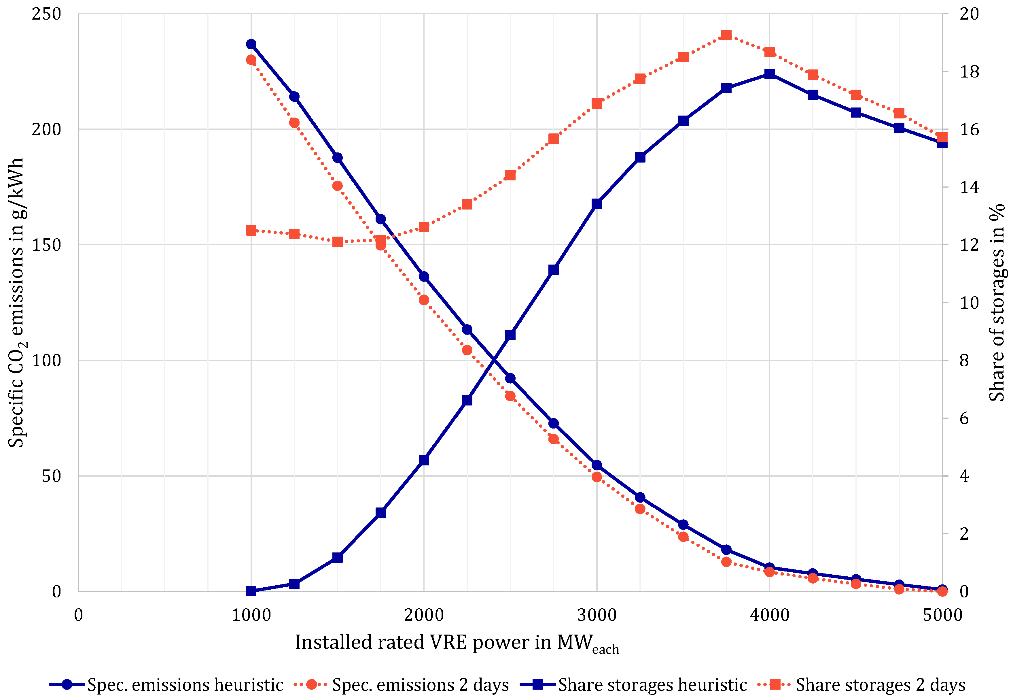
In a first step, the usage of the UCH is compared to the UCO with 2 days interval rolling horizon (scenario a) for all VRE power configurations. Figure 6 shows the specific CO₂ emissions (dots) of the plants of the copper plate island and the storage share (square) in dependence on installed VRE power. The results show that the UCO model (dotted lines) leads to slightly lower CO₂ emissions than the UCH (solid lines) for all configurations.

In terms of the storage share, the UCO delivers a widely different result than the UCH, with higher values in all configurations but especially for small installed VRE power. This is further discussed in Section 3.1. Both UCH and UCO show a maximum share of storages below the maximum installed VRE power. This is due to the ever-rising share of direct VRE supply, leaving less demand to be covered by the energy storage devices.

Lastly, Figure 6 explains why the 1000 MW_each configuration shows a lower absolute improvement than the 2000 MW_each configuration, with the storage share of the UCH. Since the UCH only integrates surplus of VRE power supply, it is obvious that the 1000 MW_each configuration has negligible surplus of VRE to be integrated, thus the UCO has only the CCGT left to optimise. In practice, this is done using the short-term storage.

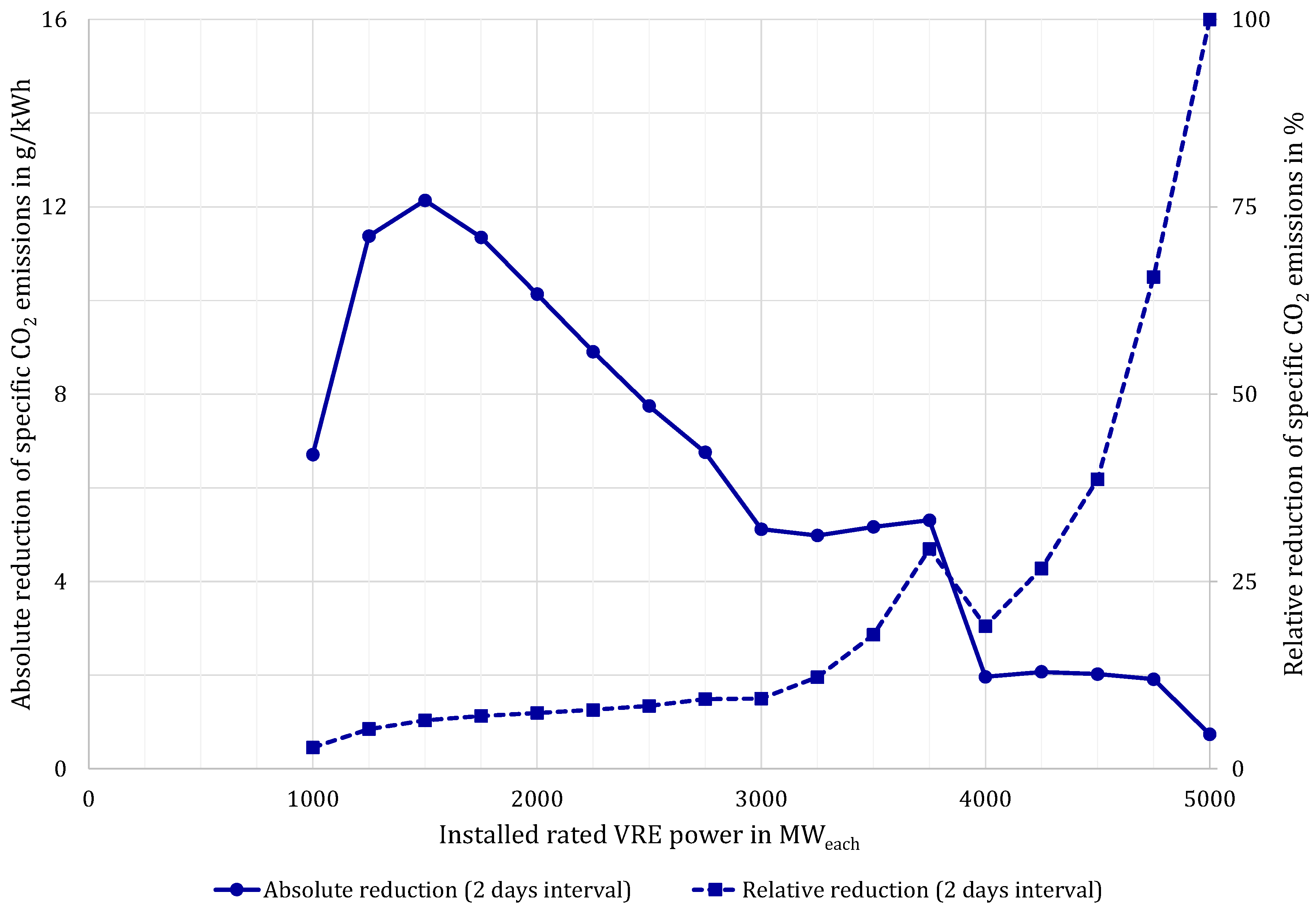
The reduction of CO₂ emissions due to optimisation in comparison to the UCH is shown in absolute and relative terms in Figure 7 also for the interval length of two days. The figure shows that the relative CO₂ reduction through UCO for installed VRE power below 3000 MW_each is generally below 10%. Between 3000 and 3750 MW_each the absolute reduction is rather constant across VRE configurations while the relative reduction shows increasing values. For 4000 MW_each both absolute and relative reduction show lower values, which can be explained with the maximum share of storage to be integrated as seen in Figure 6 and discussed above. For higher installed capacities, the denominator becomes so insignificant that the relative reduction is amplified while the absolute CO₂ reduction becomes remarkably small.

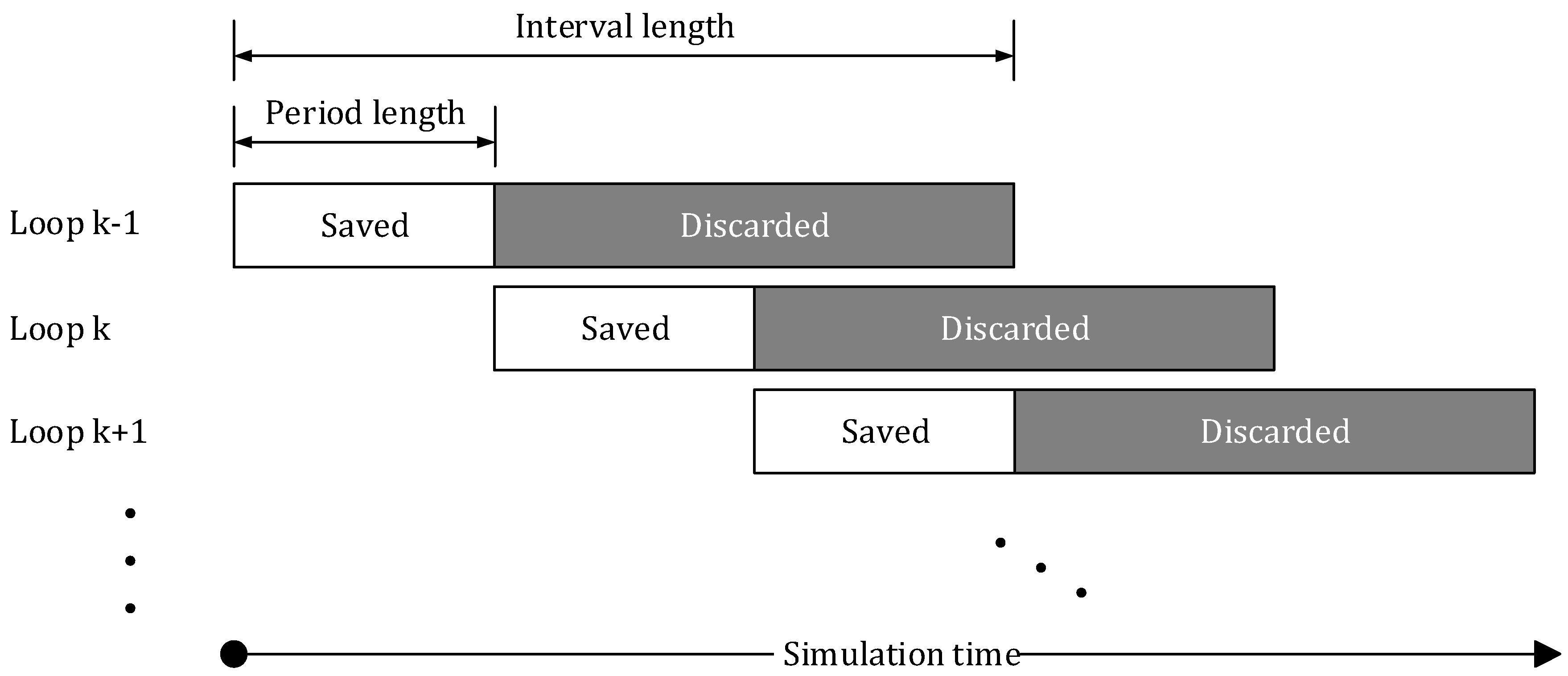
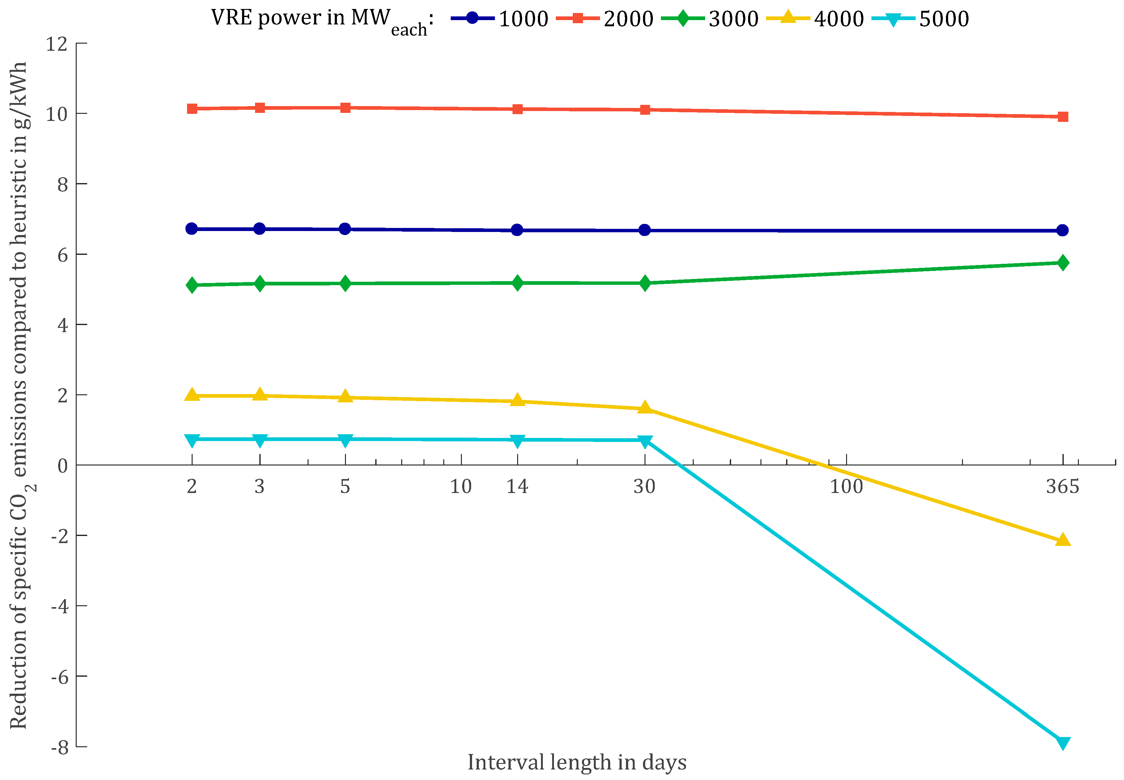
The main result can be seen in Figure 8, where the reduction of CO₂ emissions through UCO relative to the heuristic approach (UCH) is shown in relation to the interval length, which in this context implies the corresponding period lengths of Table 1. The configurations with 1000 MW_each (circles) and 2000 MW_each (squares) VRE power show no significant influence of the interval length across the scenarios (interval lengths). The configuration with 3000 MW_each shows a slight advantage for a whole year optimisation run, which is explicable with the maximum possible integration of storage power (see Figure 6) for the assumed residual power units’ configuration. For the 4000 and 5000 MW_each configurations the whole year optimisation run shows, against expectations, negative emission reduction, which can be explained by the linearisation effects, that are discussed in Section 3.2 and visible in Figure 10.

All interval lengths between 2 and 30 days with their corresponding period lengths do not seem to have a major influence on the quality of the optimisation result, but show significant changes in computational time (see

Table A3. Specific CO₂ emissions for simulated scenarios.

Installed Power Wind and Solar in MW Each	Specific CO2 Emissions in g/kWh
	Heuristic	2 Days	3 Days	5 Days	14 Days	30 Days	Year
1000	236.77	230.06	230.06	230.07	230.10	230.10	230.11
1250	214.13	202.76	-	-	-	-	-
1500	187.69	175.55	175.53	-	-	-	-
1750	161.06	149.72	-	-	-	-	-
2000	136.29	126.16	126.13	126.13	126.17	126.19	126.39
2250	113.34	104.43	-	-	-	-	-
2500	92.26	84.51	84.48	-	-	-	-
2750	72.71	65.95	-	-	-	-	-
3000	54.64	49.52	49.48	49.47	49.46	49.46	48.88
3250	40.72	35.74	-	-	-	-	-
3500	28.87	23.70	23.65	-	-	-	-
3750	18.08	12.77	-	-	-	-	-
4000	10.31	8.35	8.34	8.39	8.50	8.71	12.48
4250	7.74	5.67	-	-	-	-	-
4500	5.24	3.22	3.20	-	-	-	-
4750	2.92	1.00	-	-	-	-	-
5000	0.74	0.00	0.00	0.00	0.02	0.03	8.59

in Appendix A). Further, the graph shows that the absolute reduction of emissions through UC decreases with increased VRE power installation, the exception being the 2000 MW_each configuration, as discussed above.

3.1. Result of Unit Commitment

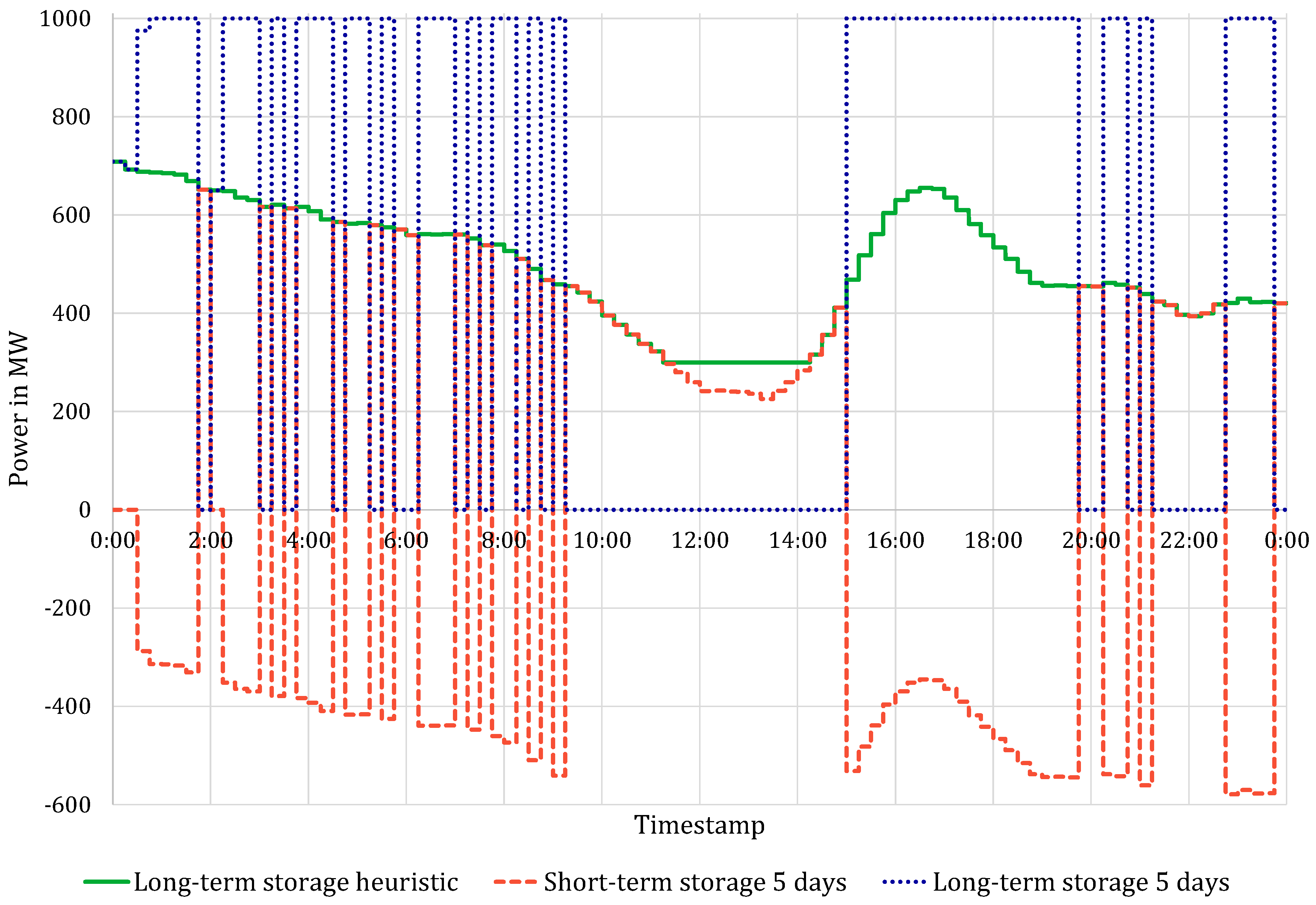
The goal of optimisation is to find non-trivial solutions [44]. Figure 9, depicting a time series excerpt, clearly shows a non-trivial result from the implemented UCO model (dashed and dotted lines). For the UCH the long-term storage device’s discharge unit (solid line) follows the residual load as the UCH emptied the short-term storage device already at that time frame (therefore not shown), which results from the pre-set order of operation. For the hours 11:30 to 14:15 however the long-term storage device’s discharge unit cannot go below its minimum load and therefore feeds to the grid with minimum load, creating the need for curtailment. The UCO makes a better use of storage devices in that the long-term storage (dotted line) rarely follows the residual load, but rather is running mostly at full power or not at all. The short-term storage device (dashed line) is charged with the surpluses created by the long-term storage device and discharges when the long-term storage device is not utilised. This happens predominantly at low residual loads, where the long-term storage device’s discharge unit would have a relative efficiency lower than the round-trip efficiency of the short-term storage device. While this seems an unrealistic unit dispatch, it is the most efficient plan, in energy terms, for the formulated mathematical problem. Hence, this can be considered an optimal strategy—especially as the curtailment due to minimum load of the long-term storage device’s discharge unit is avoided. In Figure 9, a scattering of the UC can be observed and is deemed unrealistic. It can be prevented by including intertemporal constraints such as minimum downtimes and start-up times in the mathematical problem formulation, which has not been implemented in the UCO version used in this paper. The resulting scattering of the tactic is further discussed in Section 4.

As previously discussed, the biggest difference between the UCO and the UCH can be seen in the share of storage in the supplied energy. This results from the different use of the energy storage devices. While the UCH only stores surpluses of renewables, the optimisation finds non-trivial solutions where the CCGT of the long-term storage is used at its best efficiency, charging the battery to avoid a less efficient operating point later and instead discharging the battery. This is the expected behaviour of the optimisation routine, since its target is to minimise the CO₂ emissions and the efficiency spread of the CCGT between minimum and maximum operating point is 20%-rel. and the losses due to battery usage lie around 10%.

3.2. Results for Different Interval Lengths

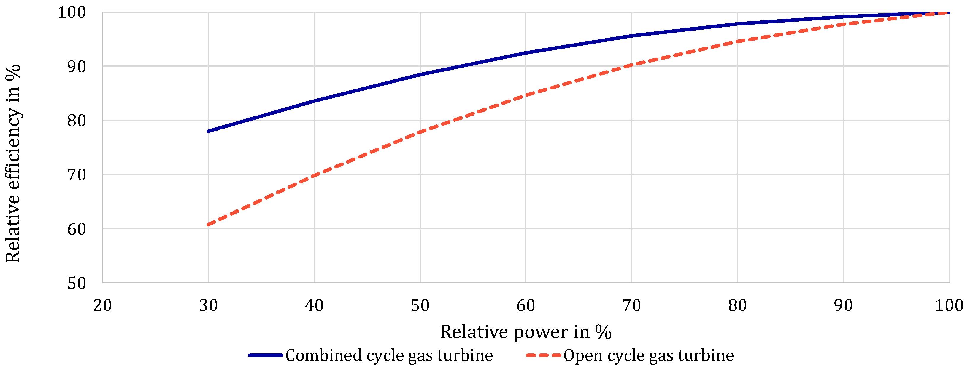
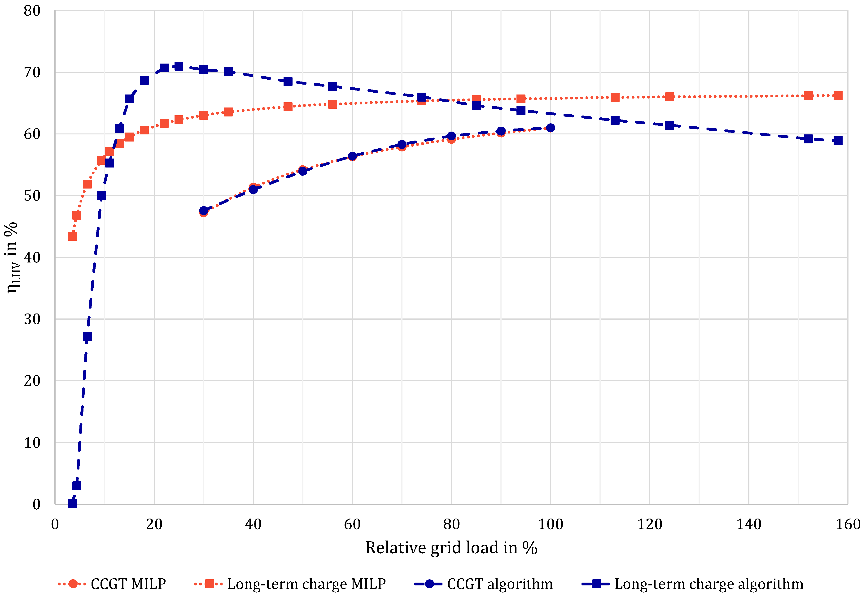
As described in Section 3.1, the characteristic line model acts as an NLC for the optimised operation plan. While the algorithm tries to set the power of each unit according to plan, it does not use the linearised efficiency curves shown in Figure 5 as dotted lines, but the non-linear characteristics (dashed lines). This results in differences between the direct MILP solution and the final UCO solution after non-linear control by algorithm.

For storage units that means that the storage level might be over- or underestimated and the unit is not running with the planned power or, due to those discrepancies in storage level, at all. For the conventional residual unit, the difference results in only negligibly different emissions when running as planned. Due to the storage deviations unplanned run-times may occur for the conventional units. These run-times result e.g., from timesteps, where the MILP can use the energy storage devices because of non-zero SOC, but the NLC calculated zero SOC (see Figure 10) and needs to use the conventional power plants to cover the residual load. The timesteps and duration of the different run-times vary with interval and period length of the rolling horizon.

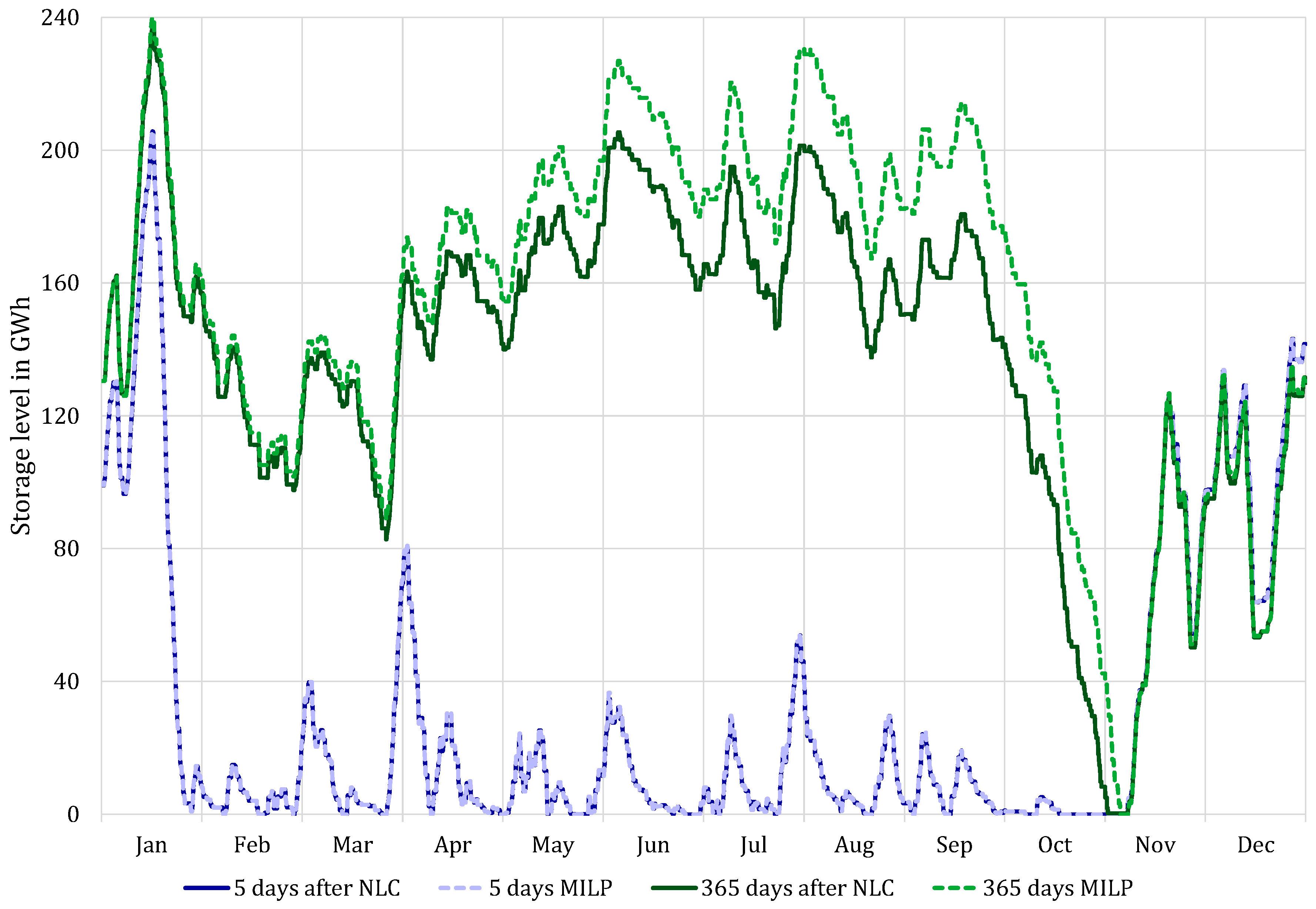
For a closer look, time series of the storage level are shown in Figure 10 for the long-term storage with an installed VRE power of 3000 MW_each. The dashed lines represent the MILP results, while the solid lines show the storage level after the NLC. The time series are presented for a 5 days interval (scenario c, blue lines) and a 365 days optimization (scenario f, green lines).

It can clearly be seen, that the storage level behaviours for both scenarios differ widely, especially from the end of January to November. In case of the 5 days interval, the storage is discharged completely at the end of January. Afterwards, the energy in the storage is charged only up to 80 GWh of energy once, with various other minor peaks, but no significant accumulation of energy. Lastly, starting in November, enough renewable surplus leads to an accumulation of energy, until the initial storage level is either reached or exceeded again.

In the 365 days interval, with perfect foresight for the entire time frame, the long-term storage is not depleted at the beginning of the year, but operated between 50 and 90% SOC. The peaks throughout the year, however, qualitatively correspond to the 5 days interval time series. After a complete discharge at the end of November, both scenarios progress with an almost equal storage level.

Furthermore, it can clearly be seen that a significant difference in storage level is mounting up as long as the zero SOC point is avoided by the MILP solution. The reason lies in the parameterisation of the long-term charge unit efficiency curve, as displayed in Figure 5. The optimiser calculates a 13 rel.-% higher efficiency for maximum power than the NLC, which in return accumulates a higher storage level for long operating hours at higher charging power (see Figure 10). As Figure 5 suggests we observe an underestimation for operating hours at low charging power.

When looking at the same VRE configuration, but shorter interval length of 5 days (blue lines) the differences in storage level between the MILP solution and the solution after NLC become significantly smaller. This is due to the rolling horizon, which is aligning the optimisation storage level more frequently (at the end of each optimisation period for a new interval) with the NLC results. For the 365 days interval and period length, there is no feedback loop, so that differences can accumulate (see Figure 10).

This is also the main cause why seemingly optimal solutions for long optimisation intervals might be found, but are not necessarily feasible by the non-linear control calculation and therefore lead to higher emissions than even the simplest heuristic approach.

While the linearisation effects mainly influence scenarios with long optimisation intervals (in this paper especially the 365 days optimisation in scenario f), the VRE configuration influences the magnitude of those effects. With higher installed VRE capacity, the usage of the long-term storage with high loads increases, so that higher deviations due to linearisation effects can accumulate. This can be observed in Figure 8.

4. Discussion

Several points need to be discussed in order to correctly categorise the findings of this paper. As previously stated, the constant power demand does not represent a real grid situation. The complexity still was deemed sufficient for the test of interval lengths, which is supported by Figure 9, where the UCO comes to a different solution than the UCH in almost every time step. The quantitative values of specific emissions and storage share therefore do not represent a prognosis for future energy systems. Additionally, it is emphasized, that the configuration of residual power supply was not optimised. Lastly, with the chosen boundary conditions it could be argued, that either the efficiency curves or the number of units should have been adjusted to correctly represent the installed powers. This was deemed too complex within the scope of this research.

The linearisation effects presented in Section 3.2 can mainly be attributed to the efficiency curve parameterisation in Section 2.6.3. A different formulation of the optimisation target might resolve in a closer fit around maximum power. The results for high installed VRE power might be improved by that. An adjustment of the parameter optimisation’s objective (see Equation (15)) was not done however, since the 365 days interval is considered unrealistic and other interval lengths were matching the NLC’s result close enough (see Figure 10). This rather shows the missing robustness of a 365 days interval length for the chosen problem.

A shorter period length for the 365 days interval might fix the previously mentioned problems, but that was considered too distant from the scope of this paper due to large computational effort. In general, the results for the different interval lengths might be tied closely to the corresponding period lengths. This difference is only addressed by the 2 and 3 days interval lengths, where no significant effect occurred.

Another point that needs discussion is the scattering observed in Figure 9. The CCGT of the long-term storage is working for several short time periods following each other rather closely. This is a behaviour that would not be expected in reality since there are temporal constraints on down-time and maximum possible ramps to consider. This was deemed beyond of scope for this paper, but will be worked on to better approximate real behaviour. As it is expected to change the results only in quantity and appearance it is seen as a minor problem for the findings of this paper.

As a last shortcoming of the model it should be emphasized, that the implemented heuristic is very simple. It could be argued that a more complex heuristic of conditions and loops could meet the results of the optimisation more closely. A rather simple heuristic was chosen, since the results were meant to cover the baseline expectation.

5. Conclusions

In this paper, a different modelling approach for rolling horizon UC was presented. For that approach, a UCO model was implemented and its positive effect in contrast to a simple UCH could be clearly shown. As the main result it is observed, that the interval length for a rolling horizon approach has an almost negligible effect on the objective value, namely the CO₂ emissions of the energy park, with this approach, even though, the detailed unit commitment can vary significantly (see Figure 10)). However, the difference is mainly to be found in computational effort.

A 2 days optimisation interval is therefore suggested as sufficient considering quantitative reduction of the optimisation target, computation time (see solver statistics in the Appendix A) and realistic lengths of weather forecasts [42,43].

The variation of the configuration (installed volatile power capacity in this study) however has a bigger effect on the optimisation objective (CO₂ emissions in this study) than the UCO. Considering the massive computation time of a UCO, it is suggested to explore configuration variations using a simple heuristic and to optimise a small set of resulting configurations with a UCO only afterwards.

The effects of the linearisation of a given system as discussed in Section 4 make a strong case for rolling horizon and against whole-year optimisation runs. Additionally, a system configuration optimised according to a whole year optimisation run might lead to different results than a system configuration optimised according to a rolling horizon run. Since the forecast length that is inherent to a whole year run is not achievable, it is suggested to optimise an energy system configuration with a rolling horizon approach as the final configuration of any energy system should work with realistically achievable foresight.

Outlook

While the proposed optimisation model already allows a detailed technical description of the energy system, there are several possibilities for model improvement in upcoming versions. As discussed in Section 4, the optimiser’s results tend to include scattering of generation and storage units. Intertemporal constraints could resolve that problem. Such intertemporal constraints will be included and looked upon in future versions. It is of great interest how that effects both the solution and the computation time since the problem is more complex but also tighter, which might make the decision trees of the branch-and-bound considerably smaller.

In this paper, the optimisation goal is set to minimise the CO₂ emissions of the underlying energy system. Another common approach is the minimisation of (operational) costs, which is currently being implemented allowing multi-objective optimisations (costs and CO₂ emissions).

A major problem with using a rolling horizon for UC problems is the control of storage levels for long-term storages, especially with short interval length, because the optimiser is not aware and therefore does not plan for eventually upcoming periods of continuously low supply of VRE power (“dark doldrums”). The use of long-term storage strategies e.g., by the use of minimum support points is an interesting topic for investigation.

Lastly, it would be interesting to see whether the findings of this paper are applicable to different configurations and more complex systems.

References

1. United Nations. Framework Convention on Climate Change. In Adoption of the Paris Agreement; FCCC/CP/2015/L.9/Rev.1; United Nations: New York, NY, USA, 2015. [Google Scholar]
2. Buttler, A.; Spliethoff, H. Bedarf und Auslastung konventioneller Kraftwerke im Zuge der Energiewende: Eine Metastudie. VGB PowerTech 2016, 3, 41–47. [Google Scholar]
3. Sterner, M.; Stadler, I. Energiespeicher. Bedarf, Technologien, Integration; Springer: Berlin/Heidelberg, Gernamy, 2014; ISBN 978-3-642-37379-4. [Google Scholar]
4. Abujarad, S.Y.; Mustafa, M.W.; Jamian, J.J. Recent approaches of unit commitment in the presence of intermittent renewable energy resources: A review. Renew. Sustain. Energy Rev. 2017, 70, 215–223. [Google Scholar] [CrossRef]
5. Ommen, T.; Markussen, W.B.; Elmegaard, B. Comparison of linear, mixed integer and non-linear programming methods in energy system dispatch modelling. Energy 2014, 74, 109–118. [Google Scholar] [CrossRef]
6. Mehleri, E.D.; Sarimveis, H.; Markatos, N.C.; Papageorgiou, L.G. Optimal design and operation of distributed energy systems: Application to Greek residential sector. Renew. Energy 2013, 51, 331–342. [Google Scholar] [CrossRef]
7. Henning, H.-M.; Palzer, A. A comprehensive model for the German electricity and heat sector in a future energy system with a dominant contribution from renewable energy technologies: Part I: Methodology. Renew. Sustain. Energy Rev. 2014, 30, 1003–1018. [Google Scholar] [CrossRef]
8. Scholz, Y. Renewable Energy Based Electricity Supply at Low Costs: Development of the REMix Model and Application for Europe. Ph.D. Dissertation, Universität Stuttgart, Stuttgart, Germany, January 2012. [Google Scholar]
9. Sarker, M.R.; Wang, J. Unit Commitment on the Cloud. 2017. Available online: http://arxiv.org/pdf/1702.03886v1 (accessed on 13 March 2019).
10. Morales-España, G.; Latorre, J.M.; Ramos, A. Tight and Compact MILP Formulation for the Thermal Unit Commitment Problem. IEEE Trans. Power Syst. 2013, 28, 4897–4908. [Google Scholar] [CrossRef]
11. Silvente, J.; Kopanos, G.M.; Pistikopoulos, E.N.; Espuña, A. A rolling horizon optimization framework for the simultaneous energy supply and demand planning in microgrids. Appl. Energy 2015, 155, 485–501. [Google Scholar] [CrossRef]
12. Stadler, P.; Ashouri, A.; Maréchal, F. Model-based optimization of distributed and renewable energy systems in buildings. Energy Build. 2016, 120, 103–113. [Google Scholar] [CrossRef]
13. Ringkjøb, H.-K.; Haugan, P.M.; Solbrekke, I.M. A review of modelling tools for energy and electricity systems with large shares of variable renewables. Renew. Sustain. Energy Rev. 2018, 96, 440–459. [Google Scholar] [CrossRef]
14. Silvente, J.; Kopanos, G.M.; Dua, V.; Papageorgiou, L.G. A rolling horizon approach for optimal management of microgrids under stochastic uncertainty. Chem. Eng. Res. Des. 2018, 131, 293–317. [Google Scholar] [CrossRef]
15. Costley, M.; Feizollahi, M.J.; Ahmed, S.; Grijalva, S. A rolling-horizon unit commitment framework with flexible periodicity. Int. J. Electr. Power Energy Syst. 2017, 90, 280–291. [Google Scholar] [CrossRef]
16. Chen, H.; Xuan, P.; Wang, Y.; Tan, K.; Jin, X. Key Technologies for Integration of Multitype Renewable Energy Sources—Research on Multi-Timeframe Robust Scheduling/Dispatch. IEEE Trans. Smart Grid 2016, 7, 471–480. [Google Scholar] [CrossRef]
17. Schulze, T.; McKinnon, K. The value of stochastic programming in day-ahead and intra-day generation unit commitment. Energy 2016, 101, 592–605. [Google Scholar] [CrossRef]
18. Saint-Pierre, A.; Mancarella, P. Active Distribution System Management: A Dual-Horizon Scheduling Framework for DSO/TSO Interface Under Uncertainty. IEEE Trans. Smart Grid 2017, 8, 2186–2197. [Google Scholar] [CrossRef]
19. Hermans, M.; Bruninx, K.; Delarue, E. Impact of CCGT Start-Up Flexibility and Cycling Costs Toward Renewables Integration. IEEE Trans. Sustain. Energy 2018, 9, 1468–1476. [Google Scholar] [CrossRef]
20. Bischi, A.; Taccari, L.; Martelli, E.; Amaldi, E.; Manzolini, G.; Silva, P.; Campanari, S.; Macchi, E. A rolling-horizon optimization algorithm for the long term operational scheduling of cogeneration systems. Energy 2017. [Google Scholar] [CrossRef]
21. Brijs, T.; Geth, F.; Siddiqui, S.; Hobbs, B.F.; Belmans, R. Price-based unit commitment electricity storage arbitrage with piecewise linear price-effects. J. Energy Storage 2016, 7, 52–62. [Google Scholar] [CrossRef]
22. Lopion, P.; Markewitz, P.; Robinius, M.; Stolten, D. A review of current challenges and trends in energy systems modeling. Renew. Sustain. Energy Rev. 2018, 96, 156–166. [Google Scholar] [CrossRef]
23. Breithaupt, T.; Leveringhaus, T.; Hofmann, L. Heuristic solution of a joint electric control reserve and wholesale market model. Int. J. Model. Simul. Sci. Comput. 2018, 1940001. [Google Scholar] [CrossRef]
24. Li, B.; Roche, R.; Miraoui, A. Microgrid sizing with combined evolutionary algorithm and MILP unit commitment. Appl. Energy 2017, 188, 547–562. [Google Scholar] [CrossRef]
25. Marquant, J.F.; Evins, R.; Carmeliet, J. Reducing Computation Time with a Rolling Horizon Approach Applied to a MILP Formulation of Multiple Urban Energy Hub System. Procedia Comput. Sci. 2015, 51, 2137–2146. [Google Scholar] [CrossRef]
26. Wolf, D.; Witt, M.; Bruckner, T. Auswirkung der fluktuierenden Stromeinspeisung aus Windenergie auf die CO2-Emissionen fossil befeuerter Kraftwerke. In Energiesysteme der Zukunft: Technologien und Investitionen Zwischen Markt und Regulierung 5; Internationale Energiewirtschaftstagung: Wien, Austria, 2007. [Google Scholar]
27. Kehlhofer, R. Combined-Cycle Gas & Steam Turbine Power Plants, 3rd ed.; PennWell: Tulsa, OK, USA, 2009; ISBN 9781593701680. [Google Scholar]
28. IBM ILOG CPLEX Optimization Studio; IBM: New York, NY, USA, 2017.
29. Hultberg, T.H. FLOPC++ An Algebraic Modeling Language Embedded in C++. In Operations Research Proceedings 2006; Waldmann, K.-H., Stocker, U.M., Eds.; Springer: Berlin/Heidelberg, Germany, 2007; pp. 187–190. ISBN 978-3-540-69994-1. [Google Scholar]
30. 50 Hertz. Archiv Photovoltaik. Available online: http://www.50hertz.com/de/Kennzahlen/Windenergie/Archiv-Photovoltaik (accessed on 12 July 2018).
31. 50 Hertz. Archiv Windenergie. Available online: http://www.50hertz.com/de/Kennzahlen/Windenergie/Archiv-Windenergie (accessed on 12 July 2018).
32. Amprion. Einspeisung von Photovoltaik. Available online: https://www.amprion.net/Netzkennzahlen/Photovoltaikeinspeisung/index-3.html (accessed on 12 July 2018).
33. Amprion. Einspeisung von Windenergie. Available online: https://www.amprion.net/Netzkennzahlen/Windenergieeinspeisung/index-3.html (accessed on 12 July 2018).
34. Tennet. Tatsächliche und Prognostizierte Windenergieeinspeisung. Available online: http://www.tennettso.de/site/de/Transparenz/veroeffentlichungen/netzkennzahlen/tatsaechliche-und-prognostizierte-windenergieeinspeisung (accessed on 12 July 2018).
35. TransnetBW. Erneuerbare Energien: Einspeisung Fotovoltaik. Available online: https://www.transnetbw.de/de/transparenz/marktdaten/kennzahlen (accessed on 12 July 2018).
36. TransnetBW. Erneuerbare Energien: Einspeisung Windenergie. Available online: https://www.transnetbw.de/de/transparenz/marktdaten/kennzahlen (accessed on 12 July 2018).
37. Tennet. Tatsächliche und Prognostizierte Solarenergieeinspeisung. Available online: http://www.tennettso.de/site/de/Transparenz/veroeffentlichungen/netzkennzahlen/tatsaechliche-und-prognostizierte-solarenergieeinspeisung_land (accessed on 12 July 2018).
38. Netztransparenz. EEG-Anlagenstammdaten 2016. Available online: https://www.netztransparenz.de/EEG/Anlagenstammdaten (accessed on 12 July 2018).
39. Blyr, A.; Sigala, C.; Amatucci, G.; Guyomard, D.; Chabre, Y.; Tarascon, J.-M. Self-Discharge of LiMn2 O 4/C Li-Ion Cells in Their Discharged State Understanding by Means of Three-Electrode Measurements. J. Electrochem. Soc. 1998, 145, 194–209. [Google Scholar] [CrossRef]
40. Gurobi Optimization, L.L.C. Gurobi Optimizer Reference Manual. Available online: http://www.gurobi.com (accessed on 24 August 2018).
41. Kanngießer, A. Entwicklung Eines Generischen Modells zur Einsatzoptimierung von Energiespeichern für die Techno-Ökonomische Bewertung Stationärer Speicheranwendungen. Ph.D. Dissertation, Technische Univsersität Dortmund, Dortmund, Germany, 29 April 2013. [Google Scholar]
42. Baldauf, M.; Förstner, J.; Klink, S.; Reinhardt, T.; Schraff, C.; Seifert, A.; Stephan, K. Kurze Beschreibung des Lokal-Modells Kürzestfrist COSMO-DE (LMK) und seiner Datenbanken auf dem Datenserver des DWD No. 2.3. 2014. Available online: https://www.dwd.de/SharedDocs/downloads/DE/modelldokumentationen/nwv/cosmo_de/cosmo_de_dbbeschr_version_2_3_201406.pdf?__blob=publicationFile&v=5 (accessed on 24 July 2018).
43. Reinert, D.; Prill, F.; Frank, H.; Denhard, M.; Zängl, G. Database Reference Manual for ICON and ICON-EPS; No. 1.2.3; Deutscher Wetterdienst: Dortmund, Germany, 2018. [Google Scholar]
44. Voll, P.; Klaffke, C.; Hennen, M.; Bardow, A. Automated superstructure-based synthesis and optimization of distributed energy supply systems. Energy 2013, 50, 374–388. [Google Scholar] [CrossRef]
45. Kopp, M.; Coleman, D.; Stiller, C.; Scheffer, K.; Aichinger, J.; Scheppat, B. Energiepark Mainz: Technical and economic analysis of the worldwide largest Power-to-Gas plant with PEM electrolysis. Int. J. Hydrogen Energy 2017, 42, 13311–13320. [Google Scholar] [CrossRef]
46. Fuchs, G.; Lunz, B.; Leuthold, M.; Sauer, D.U. Technology Overview on Electricity Storage. Overview on the Potential and on the Deployment Perspectives of Electricity Storage Technologies; ISEA: Arlington, VA, USA, 2012. [Google Scholar]
47. Peniche Garcia, R. Analysis of Renewable Energy Integration Options in Urban Energy Systems with Centralized Energy Parks. Ph.D. Dissertation, Hamburg University of Technology, Hamburg, Germany, 2017. [Google Scholar]
48. Elsner, P.; Sauer, D.U. Energiespeicher. Technologiesteckbriefe zur Analyse „Flexibilitätskonzepte für die Stromversorgung 2050. “Technologiesteckbriefe zur Analyse” Flexibilitätskonzepte für die Stromversorgung 2050. 2015. Available online: https://energiesysteme-zukunft.de/publikationen/materialien/technologiesteckbriefe-zur-analyse-flexibilitaetskonzepte-fuer-die-stromversorgung-2050/ (accessed on 23 July 2018).
Figure 1. Relative efficiency curves for combined cycle gas turbines (solid line) and open cycle gas turbines (dashed line) according to [27].
Energies 12 01003 g001
Figure 2. Simplified schematic program flow of CharL.
Energies 12 01003 g002
Figure 3. Simplified diagram of a rolling horizon with a ratio of period length to interval length of 1/3.
Energies 12 01003 g003
Figure 4. Input data for the model: solar (yellow) and wind (blue) power generation. The capacity factor represents the ratio of generated power to installed capacity.
Energies 12 01003 g004
Figure 5. Efficiency curves as used in algorithm (dashed lines) and their linearised counter parts (dotted lines) as used for MILP for CCGT (which is also long-term storage discharge) (circles), and long-term storage charge unit (squares). The linearised counterparts are generated using Equation (15) with the parameters of Table 3.
Energies 12 01003 g005
Figure 6. Specific CO2 emissions (circles) and share of storages of supplied demand (squares) for the heuristic approach (solid lines) and a UCO with a 2 days interval (dotted lines).
Energies 12 01003 g006
Figure 7. Absolute (circles) and relative (squares) reductions in CO2 emissions as a result of UCO in comparison to UCH for scenario a (2 days interval).
Energies 12 01003 g007
Figure 8. Reduction of specific CO2 emissions through UCO compared to heuristic approach for different installed VRE powers (expressed in MWeach) and interval lengths.
Energies 12 01003 g008
Figure 9. Time series excerpt of power of storages according to heuristic approach and UCO with 5 days interval on 17 January. 3000 MWeach of VRE are installed. Short-term storage power of UCH is not shown, since it is zero.
Energies 12 01003 g009
Figure 10. Time series of the storage level of a long-term storage for MILP result (dashed) and after control calculation (solid) for 3000 MWeach VRE power, using 5 days interval (scenario c, blue) and 365 days interval (scenario f, green).
Energies 12 01003 g010