Remote Monitoring of Joints Status on In-Service High-Voltage Overhead Lines

Abstract

This work presents the feasibility study of an on-line monitoring technique aimed to discover unwanted variations of longitudinal impedance along the line (also named “impedance discontinuities”) and, possibly, incipient faults typically occurring on high voltage power transmission lines, like those generated by oxidated midspan joints or bolted joints usually present on such lines. In this paper, the focus is placed on the application and proper customization of a technique based on the time-domain reflectometry (TDR) technique when applied to an in-service high-voltage overhead line. An extensive set of numerical simulations are provided in order to highlight the critical points of this particular application scenario, especially those that concern the modeling of both the TDR signal injection strategy and the required high-voltage coupling devices, and to plan a measurement activity. The modeling and simulation approach followed for the study of either the overhead line or the on-line TDR system is fully detailed, discussing three main strategies. Furthermore, some measurement data that were used to characterize the specific coupling device selected for this application at high frequency—that is, a capacitive voltage transformer (CVT)—are presented and discussed too. This work sets the basic concepts underlying the implementation of an on-line remote monitoring system based on reflectometric principles for in-service lines, showing how much impact is introduced by the high-voltage coupling strategy on the amplitude of the detected reflected voltage waves (also named “voltage echoes”).

1. Introduction

It is a matter of fact that the natural evolution toward more and more sophisticated energy systems, such as smartgrids and supergrids, is pushing the market of electrical energy and also the related handlers, namely the transmission system operators (TSO), to more advanced power line management strategies [1,2,3,4], and hence to more accurate monitoring techniques [5,6,7,8]. Even though, typically, all infrastructure built to implement the national electric transmission lines are shaped to be rugged and reliable, the extremely high and ever increasing power demands are capable of overstressing the critical parts of the entire power grid, sometimes resulting in temporary hard faults or also the breakdown of the grid itself, in this way causing a long list of obvious severe inconveniences.

It is easily understandable that due to these considerations, the necessary inherent step ahead is to research for effective and reliable monitoring techniques for power grids. This next step is supported by the fluctuating production from renewable sources and unavoidable aging of the overall electricity network.

At present, the actual status of advancement in this context is stuck in a controversial situation, where there are, on the one side, a lot of research efforts that explore a wide range of new and alternative monitoring techniques, such as the ones employing electromagnetic (EM) techniques [9,10,11,12,13,14], vibro-acoustic techniques [15], information technology (IT) solutions [16,17], and drones [17,18], whereas, on the other side, in the real-world, monitoring activity is mainly still linked with manual inspection methodologies using thermo-graphic cameras recordings [19,20].

Among the new explored pathways, some appealing approaches have been the ones based on the application of electrical reflectometric techniques, like the ones employing time-domain reflectometry (TDR), which have already been successfully applied to fault-detection and localization applications in other fields of electric and electronic systems. Based on this technique, a test signal is injected into an electric line to catch the reflected waves produced by possible impedance variations along the line. Although this technique is well established in the field of electronic applications, it is a challenging application in the field of power transmission lines. In fact, while very accurate control of the impedances (characteristic, load, etc.) is achieved in electronic systems’ TDR measurements, in the power lines domain, the parameters and impedance values experience large uncertainty. In addition to this, it is a matter of fact that power lines can spread over hundreds of kilometers and are subject to environmental variables, so it is very difficult in practice to detect impedance variations due to incipient faults, which are indeed the most common symptoms of power line degradation.

An interesting tentative strategy to apply the TDR technique to power lines was proposed in [21,22,23], where, thanks to a close collaboration with the Italian National TSO (namely, TERNA S.p.A.), the reflections of some types of artificial defects were successfully detected [21] and also types related to the intrinsic variations of the line impedance, such as transpositions [23]. The principal issue of the presented results consists in the necessity to set the power line out-of-service (OoS), which is a very important for the TSO, making the approach unaffordable for concrete real-time monitoring.

The aim of this work is to set-up a strategy to extend the basic approach presented in [21,22,23] toward in-service (IS) power lines, thus making the TDR technique more appealing from an application point of view.

In particular, in this contribution, the basic TDR strategy (OoS line case) is outlined in Section 2, showing the modeling steps that were followed to represent the high-voltage overhead line and the TDR signal injection system. In Section 3, an extension of the basic method to IS lines is discussed, highlighting the most prominent aspects related to the high-voltage (HV) coupling method. In particular, for this case study, it is assumed that HV coupling is realized through an instrument transformer, namely a capacitive voltage transformer (CVT).

All aspects regarding the high-frequency characterization of the CVT for the injection of the TDR test pulse are given in Section 3.1. Then, a proper post-processing algorithm is introduced to make the resulting data useful for the detection of defects.

The main study results are illustrated in Section 4, where the effects of the injection/measuring points are highlighted and discussed by analyzing three injection scenarios. Some preliminary conclusions are outlined in Section 5.

2. Remote Monitoring on Off-Line HV Overhead Lines

The simplest starting point to implement a monitoring strategy is an assessment of the results obtained from the TDR technique when applied to a common three-phase transmission power were been obtained in terms of the order of magnitude of the detectable impedance variations along the line and other important aspects, such as the impacts of the conductor transpositions, source to line connection, and measurement setup.

The principle underlying the monitoring technique presented in [21] for OoS power grids is the direct application of a voltage pulse, through a pulse generator owned by TERNA, at specific accessible line terminations, and then the detection of the total voltage at the same point. This voltage is a temporal combination of the injected and reflected signals due to changes of impedance, such as the line end and/or defected joints.

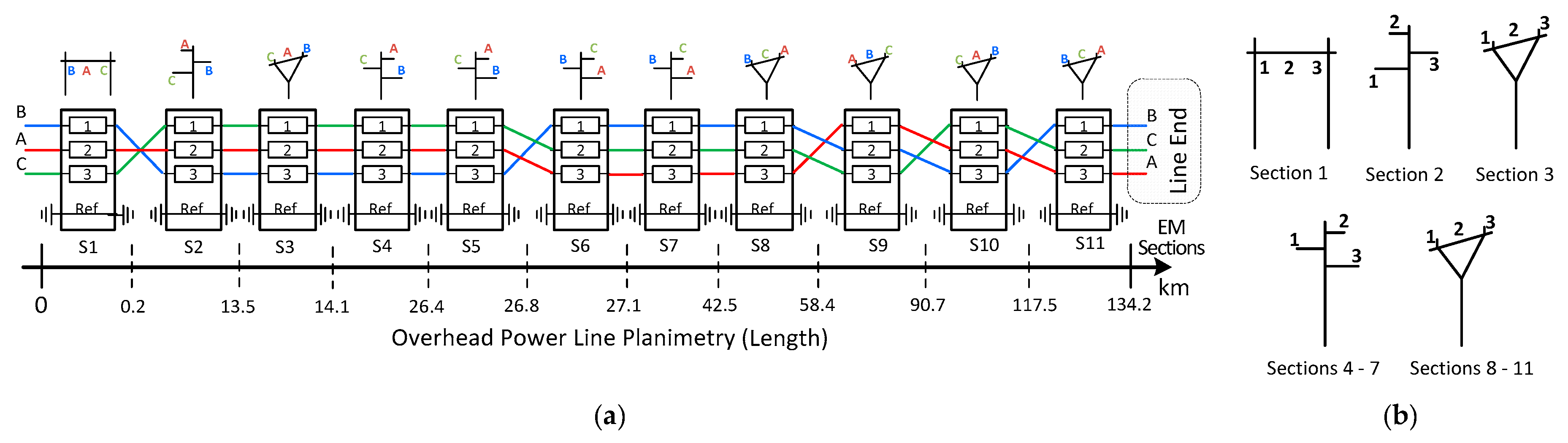
The first step is the modeling of the three-phase HV overhead power line by using the multiconductor transmission line theory [23]. The entire HV power line is decomposed in a certain set of line segments. Each line segment represents a specific part of the line, for which the conductor’s cross-section could be assumed as being approximately space-invariant.

In reference [21], a real 220 kV power line managed by the TERNA TSO was considered. This is the same line as that considered in the present study. The line was energized at 130 kV, with an effective electrical length of 134.2 km. Due to the actual layout and towers’ topology, the line was segmented into 11 sections in which the conductor’s cross-section could be assumed as being space-invariant. Figure 1a shows the longitudinal layout and Figure 1b shown the types of towers and the conductor cross section.

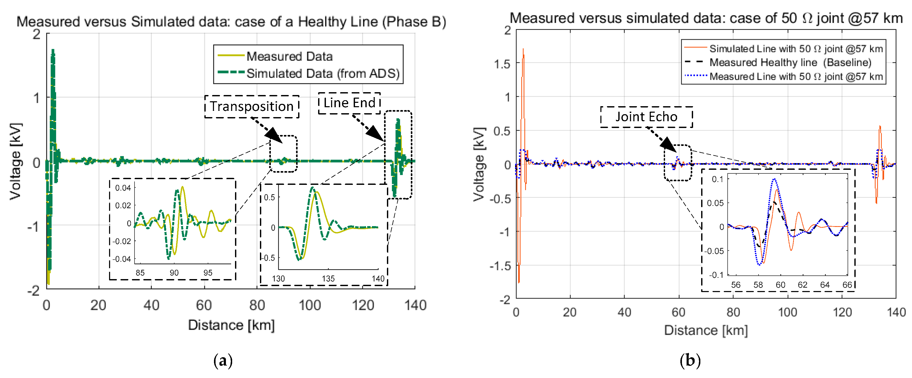
The implementation of the real TDR test bench and the measurement activities are reported in [21] and therefore are not repeated here. The effectiveness of this technique is shown by the agreement of the results obtained from a circuit simulation and the measured results as reported in Figure 2. Figure 2a shows the comparison for a line without any impedance anomaly (also named “healthy line”). Figure 2b shows the comparison for the same line where it is placed on a degraded joint with 50 impedance at the 57th km. A good agreement between the modeling and measurement is obtained.

3. Remote Monitoring on In-Service HV Overhead Lines

Even though the OoS TDR monitoring strategy is, in practice, the simplest and most convenient technique, it is also the least appealing one from an application point of view. In fact, it requires a shutdown of the power grid during the test activities. Owing to this paramount aspect, the consideration of a TDR-like technique as a power line monitoring strategy requires an inherent extension to the case of IS lines.

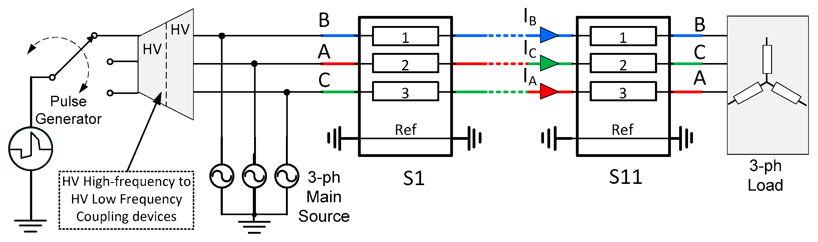
In addition to this, it should also be considered that, because of their nature, some incipient faults are naturally emphasized by the presence of loading conditions. In fact, concerning this point, it is possible to think about the case of the middle span joints’ aging problem, where the usually heavy current flow, typical of overhead lines under overstressed conditions, can produce an abnormal overheating of the joints themselves, consequently inducing in turn a further suspicious increase of the impedance related to the joints, thus making them more visible with respect to the power line bare conductors in terms of TDR voltage reflections. This section constitutes the focus of this paper, where the previously presented TDR technique for OoS lines is extended to IS lines; at a top-level, this could be represented by the principle scheme shown in Figure 3. In this scenario, the most critical and challenging points to be faced consist in the following two fundamental aspects:

• Coupling of the high-frequency test signal over the energized power line;
• Extraction of the TDR signal starting from the knowledge of the measured line input voltage.

In effect, the first main issue preventing the implementation of the TDR technique on a live power line is the capability of properly injecting a high-frequency test signal (typical of TDR-based methods) into the tested system that was specifically originally designed for low frequency applications, such as the feeding of the 50 Hz medium and low voltage electrical networks.

As already mentioned in the introductory section of the manuscript, this possibility is provided in our specific case by using a coupling device, which is an instrument transformer, namely a CVT. The other remaining issue is constituted by the fact that any classical TDR technique is intended to be applied on passive lines, but in our case, a live line is used; that is, a line with a superimposed rated supply voltage and which carries a certain amount of current (i.e., loading conditions).

From a theoretical point of view, the presence of an absorbed current does not overly affect the TDR technique. Since our case is voltage-based, the only difference is constituted (in practice) by the change of the voltage level produced by the reflected wave due to the load impedance at the end of the line. Instead, the real problem is represented by the voltage mixing effect operated by the used coupling device.

In fact, since the line is powered on, the voltage signal that can be measured at the line input terminals (for each phase) is affected by both the TDR test pulse and the rated 50 Hz voltage signal obviously present during normal line operation. It must also be said that, owing to the aim of implementing the classical TDR principle regardless of this node, the overall TDR trace (injected signal plus the possible voltage echoes) that is retrieved in this scenario would also be the composition of several voltage waves: The 50 Hz sinusoidal wave, the high-frequency pulse, and the reflections due to the line end or possible impedance change. As expected, the composition of the various signals will depend on the type of coupling device used and on the specific connection scheme realized to couple the pulse generator with the CVT.

So, it must be remarked that in the case of IS lines, a proper post-processing algorithm suitable for the retrieving the correct TDR trace information is required, which is, in this case, embedded inside the composite signal measured at the TDR injection/measurement point.

In this paper, a proposal for a simple TDR signal extraction procedure is fully illustrated in the last part of this section, which basically consists of a proper data post-processing algorithm.

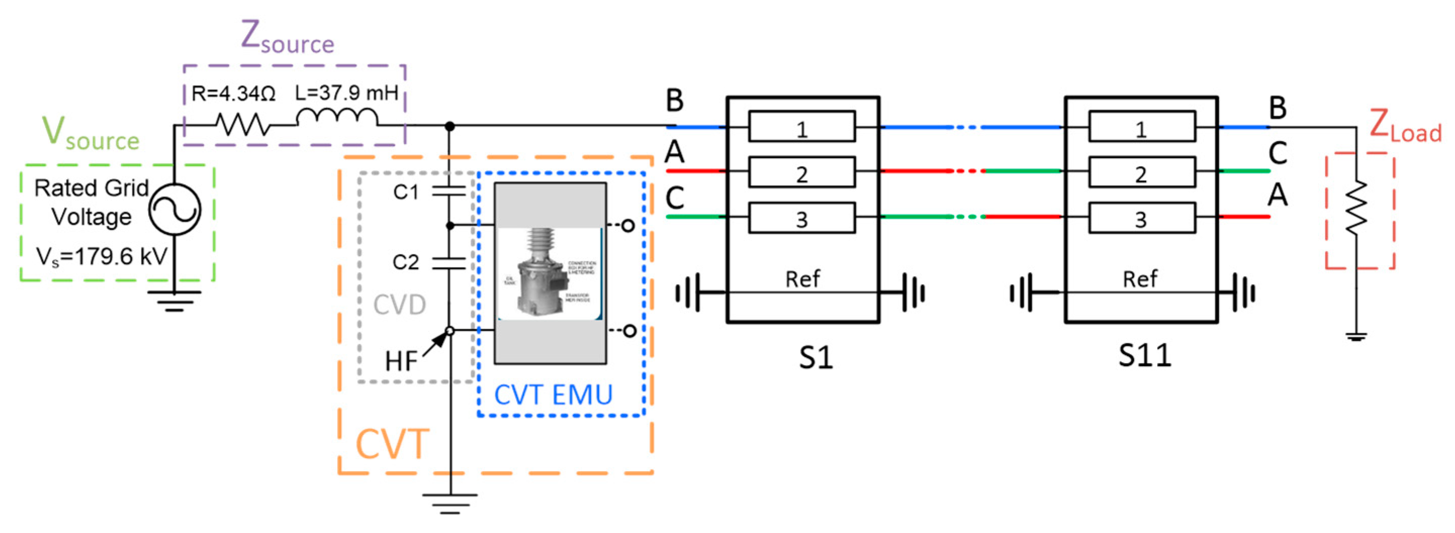
To develop both the aforementioned high-voltage coupling strategy and the post-processing algorithm, proper modeling of the IS line scenario must first be built. For the sake of simplicity, without a loss of generality, here, the study can be reduced to only one representative phase of the power grid. In this case, the developed representation is shown by the schematic representation depicted in Figure 4.

The main differences with respect to the OoS case modeling are represented by the presence of the voltage generator used for the 50 Hz sinusoidal excitation and the other following elements:

• Source impedance: It is modeled, as a first approximation, by using a proper Resistive-Inductive (RL) branch in which the values of the lumped elements were determined based on the knowledge of the short circuit current of the three-phase line. For the specific line under analysis, I_cc = 11 kA with a rated voltage of 220 kV and a phase of 75 degrees; thus, considering also the Ferranti effect, the source impedance of interest is equal to 4.34 + j 12.26 Ω, realized here through an RL branch with an R equal to 4.34 Ω and L equal to 37.9 mH.
• Load impedance: Determined by the knowledge of the rated current value for the specific line, in this case, equal to 500 [A], giving a corresponding equivalent value of Z_L = 232 Ω.
• The capacitive voltage transformer, represented in Figure 4, by highlighting its two different functional sections: The capacitive voltage divider (CVD) and the electromagnetic unit (EMU).

In this case study, we implicitly assume that no power line communication (PLC) equipment is mounted on the specific line phase of interest. Thus, the presence of other ancillary apparatus that can affect the results coming from the application of the TDR strategy can be neglected, such as, for instance, the coupling unit used for PLC applications that is usually attached to the HF terminal of CVTs, marked with “HF” in Figure 4. Normally, the HF terminal is grounded if it is not being used. For the same reasons, no line traps are accounted for in this particular application study.

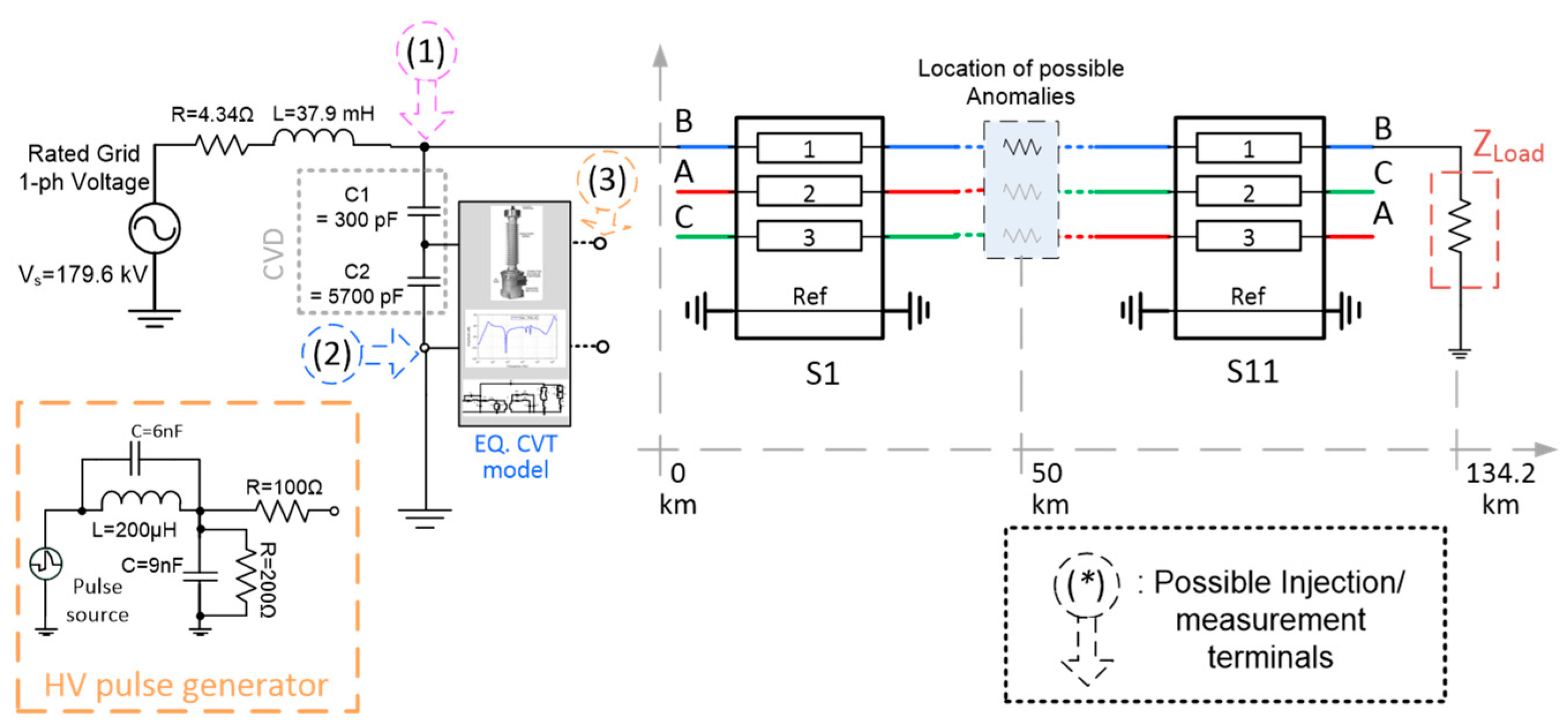
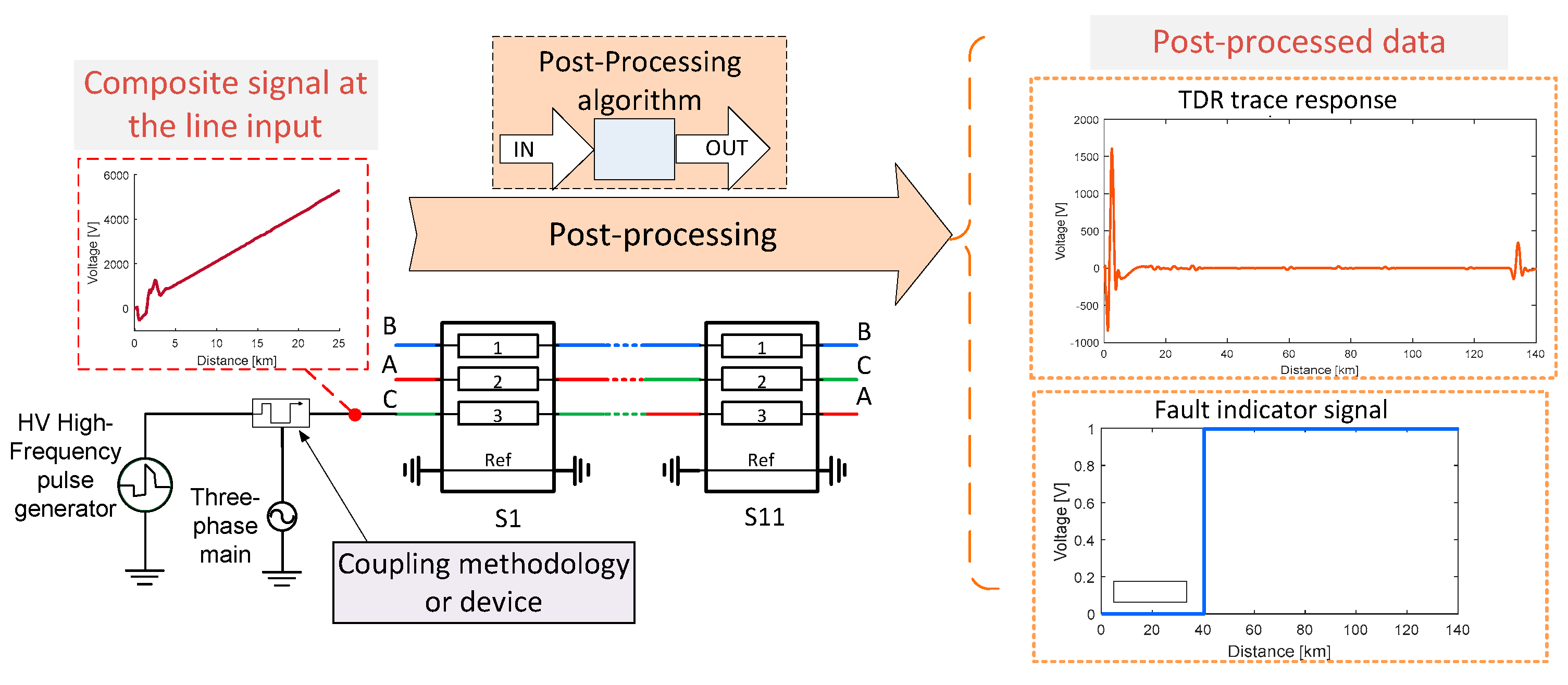
Considering the illustrated modeling of the IS line under test, the proposed approach for the TDR analysis can be stated as follows and as reported in Figure 5. That is:

• The HV TDR pulse is applied to the IS power line through the selection of proper injection/measurement terminals from among the ones available on the CVT, according to a pre-determined connection scheme (i.e., TDR injection strategy).
• The voltage signal at the selected measurement point is recorded and stored for further post-processing steps.
• The effective TDR trace response, containing the reflected voltage waves of the lumped impedance variation, is extracted from the stored signal by applying a properly designed post-processing algorithm, illustrated more in detail in Section 3.2.
• A proper fault-detection signal (“fault-indicator”) is calculated based on the knowledge of the response of the healthy line by using further steps of the data post-processing algorithm.

As a final, but fundamental, remark, it must be said that the effectiveness of the method strongly depends on the modeling of the CVT device since it constitutes the channel used to inject the TDR pulse and measure the TDR response. In addition to this, when the injection/measuring terminals are not selected to be on the secondary side of the CVT, this constitutes an electrical path capable of affecting the propagation of the high-frequency test pulse. Thus, it must be carefully characterized in terms of the frequency response. This matter is covered in the following part of this section.

3.1. Frequency Characterization and Equivalent Circuit of a CVT

From the related literature, several efforts have been aimed at obtaining an accurate representation of CVTs, both in terms of frequency characterization and/or a lumped equivalent circuit [24,25,26,27,28]. The obtainment of the latter is of great interest for the sake of circuit simulation purposes. In this study, the modeling of the CVT was done by starting from what was found in the literature, especially from [25,26], but by then customizing the equivalent circuit representation provided by theory using data from experimental measurements that were done on a real CVT effectively used for substation voltage measurement on a 132 kV overhead line. This was in effect a mint condition CVT characterized by the nameplate data reported in

Table 1. Nameplate data of the CVT under test.

Parameter	Value	Units
Rated Power 1	1000	VA
Rated Voltage	145	kV
Primary Capacitor (C1)	4286	pF
Secondary Capacitor (C2)	60,000	pF
Transformation Ratio	132/√3:100/√3	kV/V
Rated frequency	50	Hz
Insulation level	275	kV
Insulation Type	Mineral Oil	-
Mass	217	kg

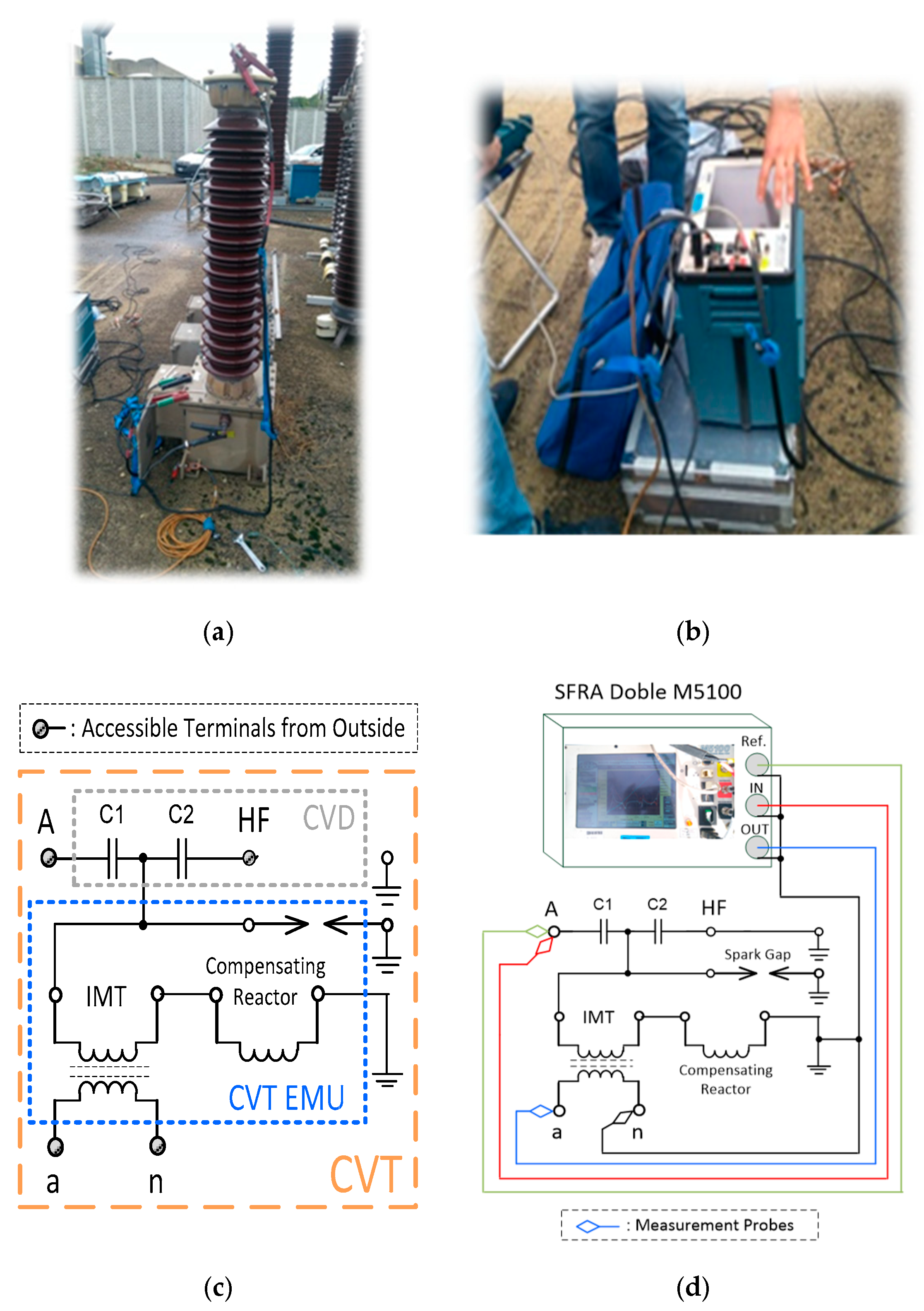
¹ Thermal rating.

, for which the frequency response was determined using sweep frequency response analysis (SFRA) measurements. A picture of the specific CVT under test is provided in Figure 6a whereas in Figure 6b, the SFRA instrument used for this purpose is depicted. It is a commercial device, namely Doble M5100, with the possibility of measuring the frequency response of the device under test from 10 Hz up to 2 MHz. At this stage, owing to the aim of determining an equivalent circuit of the CVT, which should be as general, but accurate as possible, it is very important that different measurement strategies are explored since the larger the measurement data, the better the equivalent circuit will be. However, not all the terminals of the device under test are accessible for measurement. In fact, in Figure 6c, the typical functional scheme of the CVT is shown, where only the terminals denoted with “A”, “a”, and “n” are accessible from the outside for measurement. For the sake of this work, only the measurement scheme reported in Figure 6d is considered, from which it is possible to determine the frequency response of the CVT in terms of the primary-to-secondary windings transfer function and vice versa.

Here, the basic idea is to measure the complete transfer function of the CVT and then separate the contribution due to the divider capacitors (CVD) to obtain the characterization of the EMU only. In this manner, it should be possible to also rescale the obtained model to other types of CVTs simply by adapting the CVD section in the equivalent circuit modeling stage, i.e., also to other line voltage levels. This is reasonable if it is possible to retain the EMU section as a universal and standardized part of the CVT, common to many types of commercial products, and then, considering that the CVD main function is instead the reduction of the voltage level to a standardized intermediate value (typically around 10 kV), it is suitable for use by the inductive intermediate transformer (IMT) included in the EMU.

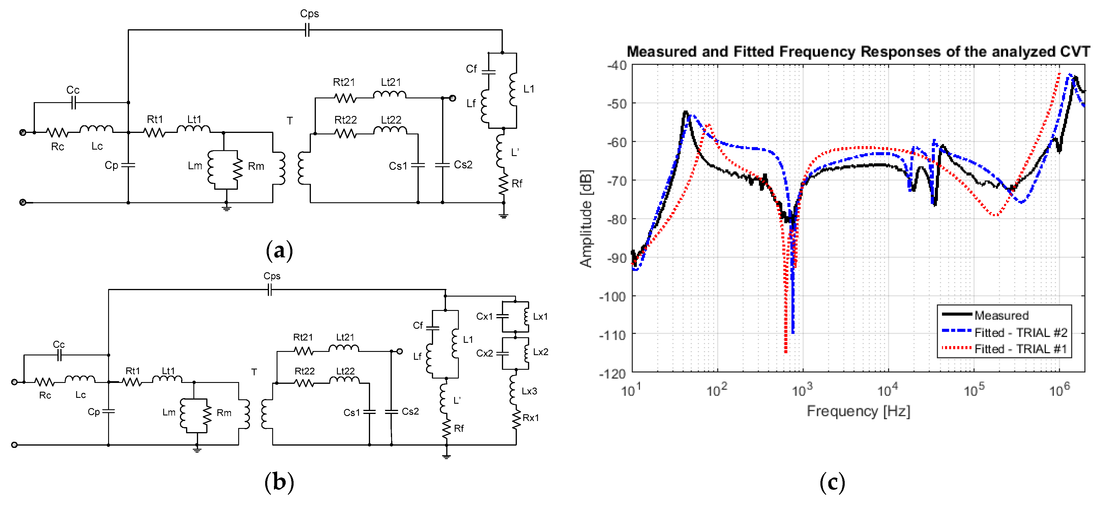
The process of extraction of the frequency response of the CVT under test allows the curve reported in Figure 7c to be obtained. It represents the transfer function from the primary side to the secondary side of the CVT. This constitutes the input data of a proper fitting procedure that is used to reconstruct the values of the lumped elements belonging to an appropriate equivalent circuit based on circuit topologies that can be found in the literature. The fitting procedure is based either on an automatic identification algorithm (implemented in MATLAB/Simulink^®) or on a manual tuning procedure (implemented following a classical trial and error workflow).

In this particular case, taking the cue from the equivalent circuit schematic exposed by [26] and applying the aforementioned fitting procedure, an equivalent circuit is able to be obtained, like the one reported in Figure 7a, which represents an initial guess of the equivalent circuit approximation that is desired. For the sake of clarity, this is indicated in the remaining of the paper as “Trial#1”.

At this point, before going into more detail, the role of the involved lumped elements must be clarified; in particular, first, the presence of an ideal transformer modeling the usual voltage transformation ratio and together with it is the other typical magnetization resistive-inductive RL branch (constituted by R_m and L_m). Moreover, the leakage impedances for the primary side (R_t1, L_t1) and the related equivalent values for the two secondary windings (R_t21, L_t21, R_t22, L_t22) also exist.

In addition to these straightforward elements, a resistive-inductive-capacitive RLC branch was also considered, aimed to take into account the presence of the CVT compensating reactor (R_c, L_c, C_c) and a proper set of capacitors modeling the likewise inherent presence of the stray capacitances of the windings, respectively: The stray capacitance of the primary winding to the ground (C_p), the stray capacitances of the two secondary windings to the ground (C_s1, C_s2), and finally, the stray capacitance between the primary and secondary windings (C_ps). The last equivalent branch included in the equivalent circuit has the role of representing the ferroresonance suppression system. It involves the elements, C_f, L_f, L₁, L’, and R_f, and was designed in a slightly different way with respect to [26]. The values of the elements used for such a kind of equivalent circuit are reported in

Table 2. Values of the lumped elements of the “TRIAL#1” equivalent circuit.

Parameter	Value	Units	Parameter	Value	Units
T	52	-	L’	0.032	H
Rm	630	kΩ	Lm	2611	H
Cc	147.3	pF	Lc	430	H
Cp	20	pF	Lt1	3.4	H
Cs1	50	pF	Rt1	400	Ω
Cs2	50	pF	Rc	228	Ω
Rf	33.4	Ω	Lf	0.084	H
Cf	0.35	μF	L1	0.111	H
Rt21	0.02	Ω	Lt21	0.317	mH
Rt22	0.02	Ω	Lt22	0.317	mH
Cps	5	pF	-	-	-

.

After this first level of approximation, another equivalent circuit topology was extracted from the measurements, in particular trying to match some resonances appearing in the frequency band between 10 and 80 kHz. Applying the same fitting procedure used for Trial#1, the obtained resulting equivalent circuit is the one reported in Figure 7b; herein, this version is referred to as “Trial#2”. The values of the elements of this second type of equivalent circuit are reported in

Table 3. Values of the lumped elements of the “TRIAL#2” equivalent circuit.

Parameter	Value	Units	Parameter	Value	Units
Cps	5	pF	T	52	−
Rm	630	kΩ	Lm	1265	H
Cc	132.8	pF	Lc	330	H
Cp	30	pF	Lt1	0.9	H
Cs1	120	pF	Lt21	0.125	mH
Cs2	50	pF	Lt22	0.063	mH
Cf	279	μF	Lf	0.25	H
Rc	219	Ω	L1	0.205	H
Rf	12	Ω	L’	0.42	H
Cx1	0.1	μF	Lx1	0.8	mH
Cx2	0.08	μF	Lx2	0.3	mH
Rx1	516	Ω	Lx3	3.35	mH

.

As can be seen from the comparison of the frequency responses obtained for the two equivalent circuits with respect to the real CVT SFRA measurement, shown in Figure 7c, it is evident that even though the second level of approximation is capable of matching the resonances encountered at 19.2 kHz and 34.7 kHz, these last two notches seem to be ascribable to secondary effects that occurred during the measurement stage. Despite this, the Trial#2 equivalent circuit can be included in the modeling stage because the two notches add no significant impairments to the actual frequency response modeling scenario.

However, in addition to this, the Trial#2 circuit is, in effect, also the one that better matches the fundamental peak response around 50 Hz, which is the most important information at the design stage for a CVT. Thus, owing to these reasons, the Trial#2 equivalent circuit is the one that is used in the following simulation analyses to study the application of the TDR technique on IS lines. In fact, it catches quite well the main CVT frequency behavior even though this is with the addition of some extra and unwanted resonant features. Furthermore, it is evident from Figure 7c that the Trial#2 equivalent circuit should also be considered because it fits for frequencies greater than 100 kHz, which are the most interesting ones owing to the aim of propagating an HF signal (like in the case of PLC communications), since the attenuation of the CVT is the lowest.

3.2. Data Post-Processing

The last stage of the proposed TDR technique for IS lines is constituted by the algorithm developed for the extraction of the TDR trace starting from the knowledge of the measured voltage signal at the line input terminals or at any other specific measurement point.

Before describing the details of the overall data post-processing procedure, it must first be said that the algorithm proposed hereafter is composed of two main parts.

In the first part, the voltage signal measured during the monitoring activity is used to compute the direct difference between the signal itself (namely “measured signal”) and the one measured (and stored) when the line is in a healthy condition, which is considered as the reference scenario (namely, the “baseline” HV line TDR response) for the detection of incipient faults and hence is used to detect the presence of degraded middle span or bolted joints. The resulting difference signal is herein referred to as “difference signal”, keeping in mind that it is the difference between the actual measured voltage signal and the respective reference baseline, but also that it will be used to compute the aforementioned “fault-indicator” signal.

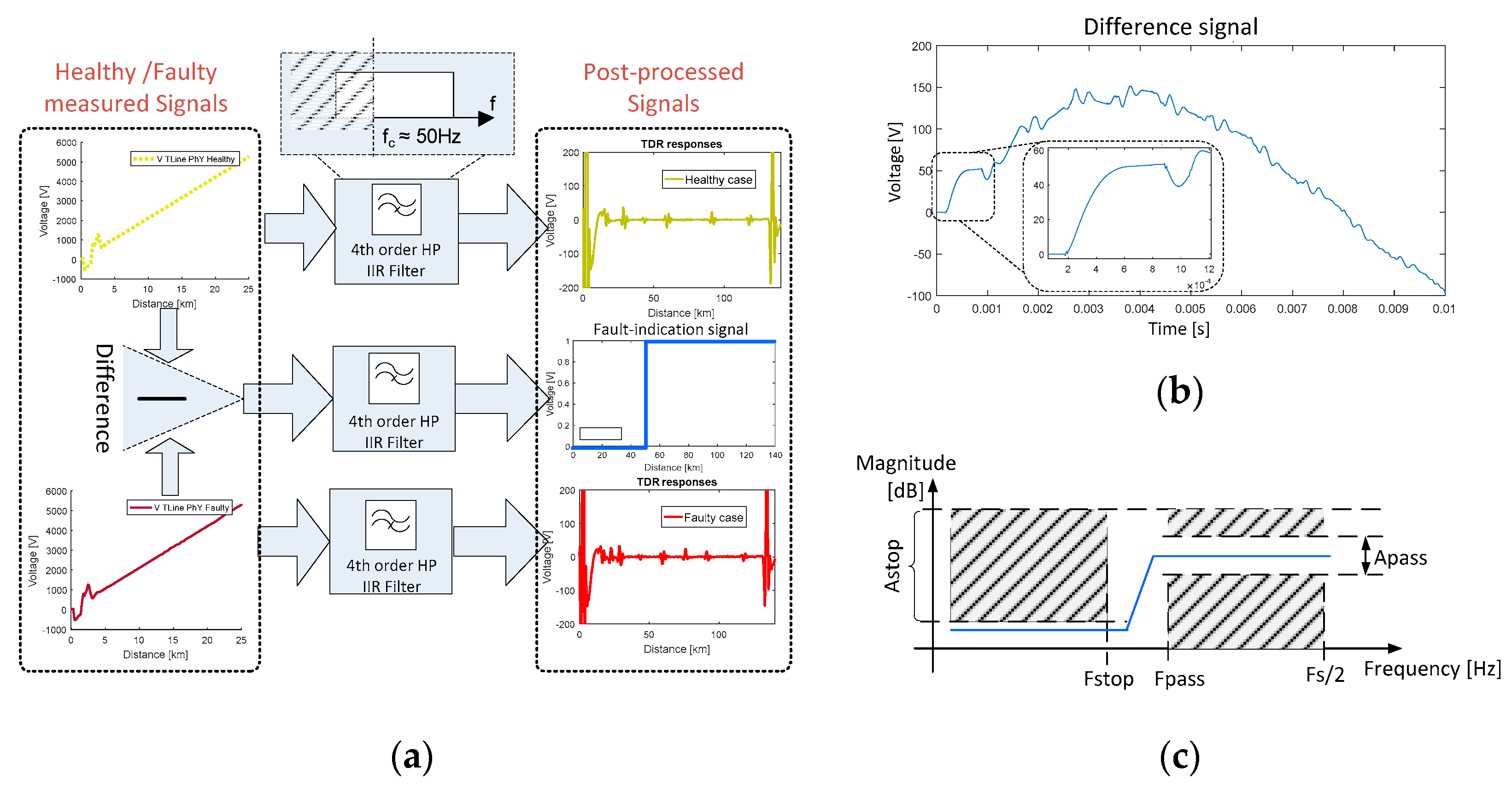
In the second part of the post-processing procedure, the measured signal and the stored reference signal (baseline) are used to compute the related TDR traces, which are carrying the information about the voltage reflections of, respectively, the impedance changes and the healthy line signature (transpositions only). Herein, they are referred to as “TDR responses”. The computation involves the use of a proper digital filtering technique to isolate the information of interest. Furthermore, the calculated difference signal is in turn also manipulated using digital filtering to give rise to the already mentioned “fault-indicator” signal, which is referred to as the “difference TDR response”. A representative scheme of the idea underlying this second part of the algorithm is reported as an example in Figure 8a.

As highlighted in Figure 8b, the difference signal is (as easily expected) very different from a classical TDR trace since it is characterized by a clear 50 Hz component still present in the dynamics of the signal itself. This can happen both in a simulation study, like this, where the difference signal is computed while having knowledge of the phase relationships between the measured signal and the stored baseline signal, and even more in a real measurement scenario, where the phase relationships are not exactly known. However, the difference signal by itself carries the information about the changes anyway, even though this last one is unavoidably embedded in it. Here, an accurate description of the filter used for the extraction of the TDR response is included, and, in particular, all the design considerations used to shape the filter response are described in the following.

Even though a huge variety of digital filters that could be used for the prescribed purpose exists—that is, in our case, the elimination of the 50 Hz signal due to the presence of the IS line supply—in this particular application case, the digital filtering technique consists of the bare application of a high-pass filter. The reasons for this are due to the fact that, at this stage of research, it was observed that the extraction of the information of the sought change of impedance (in particular its presence and position) can also be achieved with a direct high-pass filtering action, without involving too many complex algorithms. Hence, from the perspective of implementing a real on-line TDR system for in-service lines, the complexity of the overall system is required to be kept as low as possible. When the application case requires more performing techniques, then more advanced filtering algorithms are involved.

A cascade of two second order IIR high-pass digital filters of the Butterworth type were used, in particular, considering the design parameters outlined in Figure 8c. The values reported in

Table 4. Values of the design parameters implemented for the high-pass filtering algorithm.

Parameter Name	Value	Units
Fstop	50	Hz
Fpass	10	kHz
Astop	80	dB
Apass	1	dB
Fs1	10	MHz

¹ for the specific application case tested in Section 4.

were used to implement the digital filtering algorithm inside a proper computation environment; that is, in our case, the MATLAB/Simulink^® software. For the sake of clarity, the meanings of the design parameters are briefly summarized:

• Fstop: Upper value of the stopband edge frequency;
• Fpass: Lower value of the passband edge frequency;
• Astop: Minimum value of the attenuation in the stopband;
• Apass: Maximum allowable ripple value in the passband of the filter response.

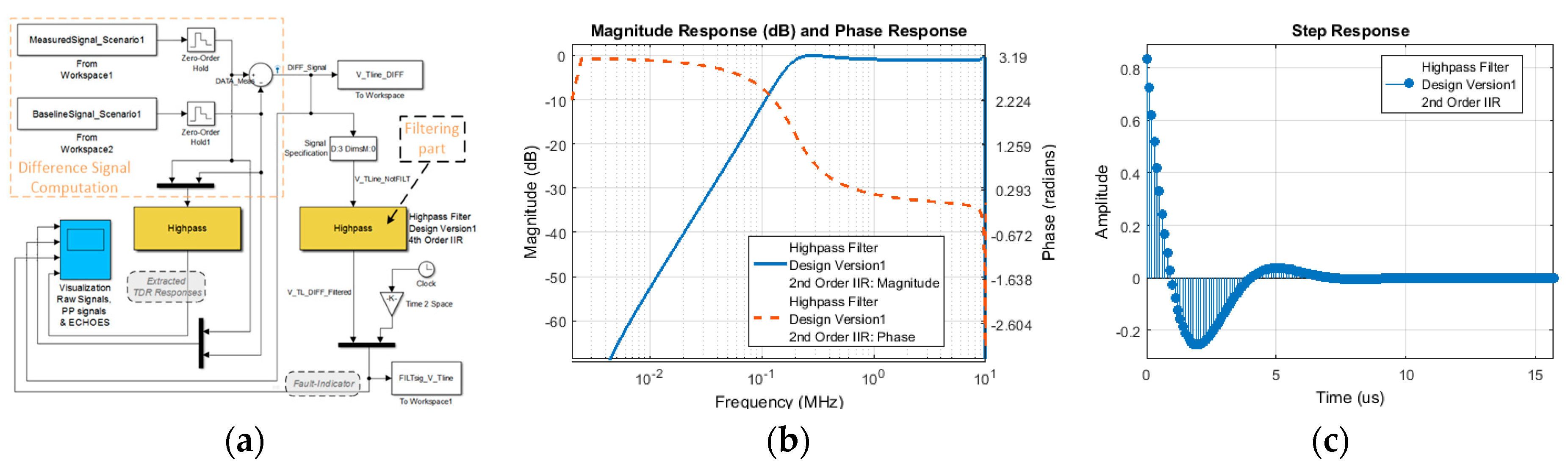
The implementation of the overall data post-processing procedure proposed in this paper takes the form of the block scheme reported in Figure 9a, where both the difference signal computation part and the filtering section are highlighted. For the sake of completeness, the frequency response of one of the two second order IIR high-pass filter sections used together with its time-domain impulse response are depicted, respectively, in Figure 9b,c.

4. Results and Discussion for Three Case Studies

Finally, the core business of this work is reported, which consists of a preliminary assessment of the TDR technique introduced in the previous section of the manuscript through an extensive simulation study. Specifically, an evaluation of the effects introduced by the choice of the injection/measurement points on the detectability of possible incipient faults using the illustrated TDR monitoring technique for in-service lines is completed.

The study is conducted through the use of numerical simulations aiming to reproduce both the healthy and degraded line cases for the 220 kV transmission power line already studied in [21,22,23], which was accurately characterized in a previous section of this paper, with a special emphasis on assessing three main application scenarios. Each one of them is related to the choice of a specific couple of injection/measurement points. 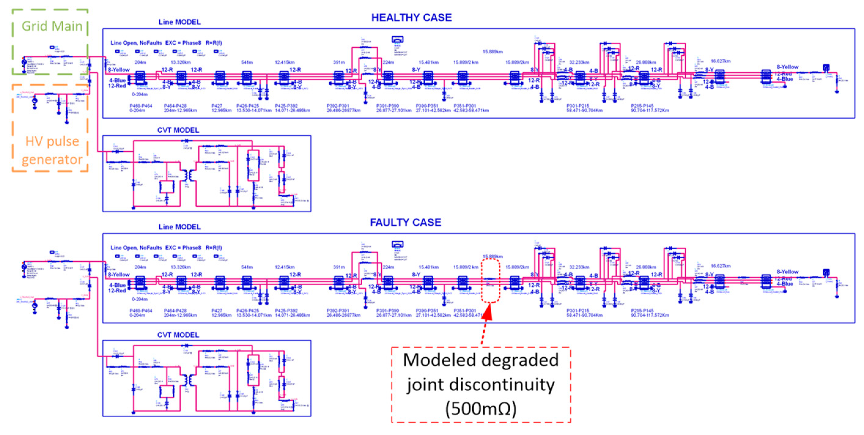Also, for this study, the circuit simulation environment used to obtain the results is Keysight Advance Design System^® (ADS^®) [29], similarly to [21,22,23]. The three aforementioned simulation scenarios are based on the schematic representation depicted in Figure 10, where the main details about the line modeling, the coupling device modeling, and the HV pulse generator modeling are reported. First, the line setup was modeled according to the indicated values expressed in Section 3, including the source impedance, the power grid 50 Hz single phase rated voltage generator (expressed as peak to peak value), and the load impedance, Z_L. Second, in Figure 10, the equivalent circuit representation that was considered to simulate the HV pulse generator source impedance is shown, which makes use of the same RLC topology identified in [23].

At this point, the CVT was simulated through the definition of specific values of the capacitors, C1 and C2, to match the real capacitances that can be found for a CVT suitable for the specific line under study, which has a 220 kV voltage level. In addition to this, the block indicated as “EQ. CVT model” was implemented using the same equivalent circuit representation detailed and discussed in Section 3.1, maintaining equal values of the lumped elements listed in Table 3 (i.e., setting the Trial#2 circuit). In Figure 10, three nodes (namely “1”,”2”, and “3”) are indicated to implement the three different injection/detection scenarios of interest in this paper.

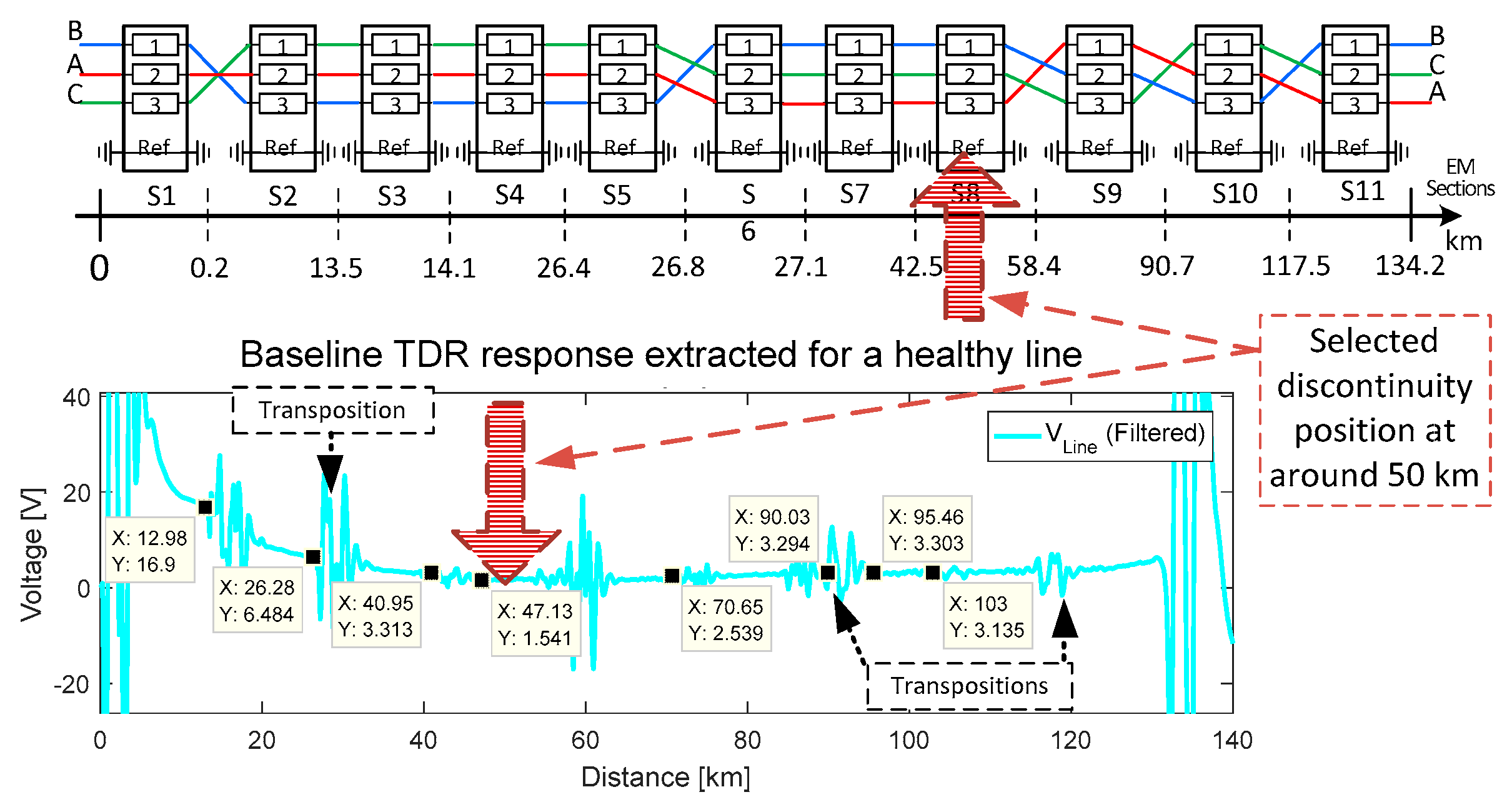
Finally, when analyzing the simulation case of a line with degraded joints, the proposed scheme must be customized by introducing a proper impedance change, which in our case was only a pure resistance with a value equal to 500 mΩ since it represents a value of anomaly one order of magnitude below the minimum value that was possible to discriminate during the real measurement campaign discussed in [21], where proper artificial lumped impedances were placed along the line. In the actual study, the anomaly was placed at around 50 km from the injection point since this represents a location where the baseline TDR response was sufficiently clear from other changes represented by the inherent line conductors’ transpositions, as highlighted from Figure 11.

It must be noticed that the baseline TDR response reported in Figure 11 represents the TDR trace that can be extracted using the approach presented in Section 3, when the line is supposed to be healthy (i.e., without degraded joints), and hence the revealed reflected voltage, ascribable only to the line geometry itself, should be considered as the intrinsic “line signature”; that is, the baseline TDR trace. Furthermore, the result reported in Figure 11 shows, at the same time, the effectiveness of the proposed strategy in recovering the high-frequency TDR information embedded inside the 50 Hz voltage wave.

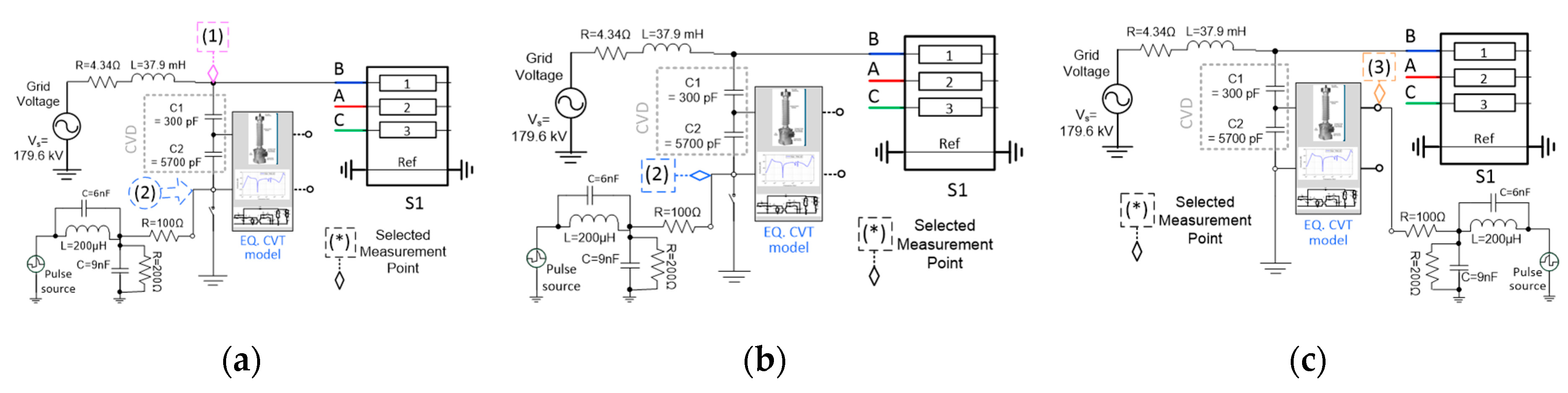
The three aforementioned study scenarios proposed in this paper to assess the impact of the injection/measurement points can be summarized as follows:

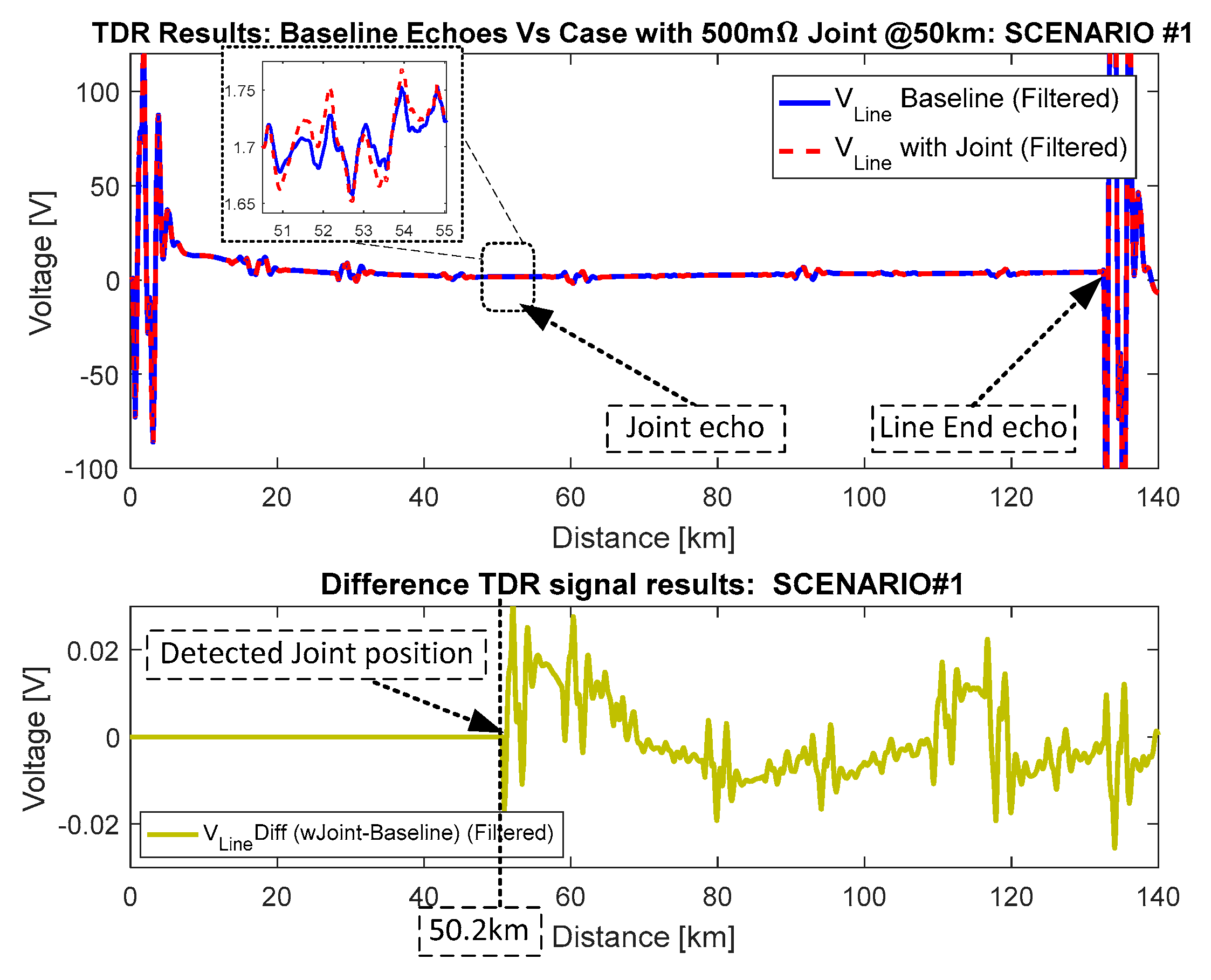
• Scenario#1: Injection of the high-frequency pulse at node “2” and measurement of the reflected voltage at node “1”; this one must be retained only as a reference case, which is not viable;
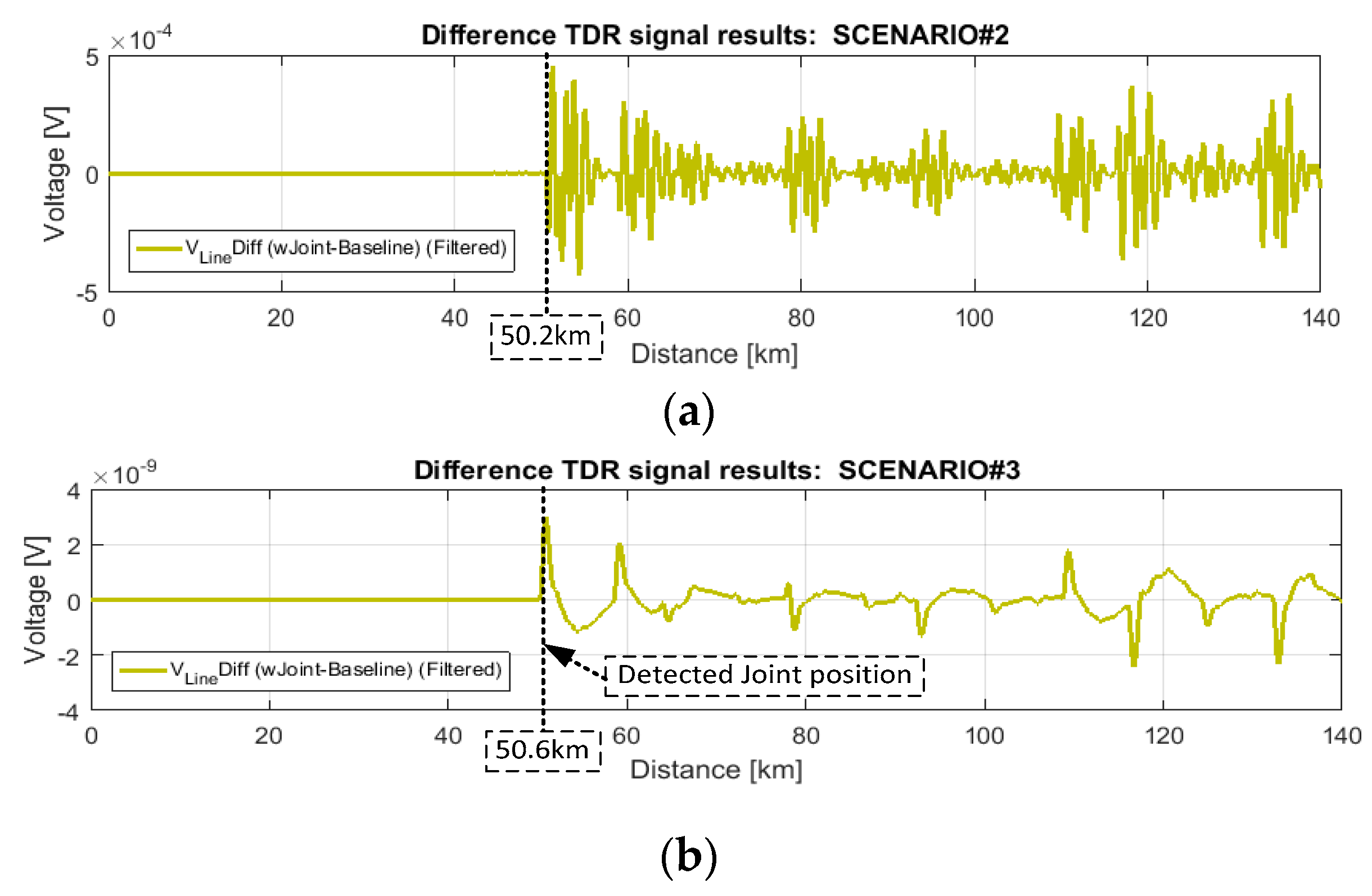
• Scenario#2: Injection of the high-frequency pulse at node “2” and measurement of the reflected voltage at the same node “2”;
• Scenario#3: Injection of the high-frequency pulse and signal detection both at node “3”.

The three circuit configurations subsequently obtained are more clearly shown in Figure 12.

Following what was already fully detailed previously in this section, the three scenarios were implemented inside the ADS simulation environment to obtain the related results. An example of what was modeled in the ADS is reported in Figure 13, in which the schematic view implemented in ADS to only simulate the case related to Scenario#1 is depicted.

Finally, the results from the three simulated scenarios are concisely reported. First, the case where the proposed TDR technique was implemented using the connection scheme of Scenario#1 is reported for an in-service line with an artificially placed lumped impedance of 500 mΩ inserted at 50 km. As a partial final outcome of this study, either the extracted TDR responses or the extracted fault-indicator one (i.e., difference TDR signal) are reported in Figure 14. As can be seen from this, the calculated difference TDR signal is zero until the impedance change position (around the 50th km) is reached, at which the signal itself experiences a maximum peak followed by a decreasing trend.

Because this study aimed to also show the results from the other two scenarios, the difference TDR signals of interest (i.e., fault-indicators) for these last two cases are reported in Figure 15. This is regardless of what was obtained for the extracted TDR responses (not differential), since the only information with a practical application comes from the analysis of the difference between the healthy case and the degraded case. Furthermore, working with the difference TDR signals gives the great advantage of removing the reflections due to the inherent impedance variations always present on the line (conductors’ transpositions), enabling the detection of small anomalies.

As can be noticed from Figure 15, the amplitude of the difference TDR signal tends to vary significantly as the connection scheme used to inject and then detect the voltage waveforms is changed according to the simulated scenario. In particular, it is observed that the smallest amplitude is assumed when using the injection/detection scheme of Scenario#3. This can be ascribed to the presence of the CVT either in the injection signal path or in the detection signal path, which acts as a strong filter, hence also reflecting the related frequency response gathered in Section 3.1. In fact, in Figure 15b, there is not only a very small amplitude of the difference TDR signal, but also a lower level of harmonics with respect to the case of Figure 15a.

Despite this detrimental effect, in theory, the detection of the degraded joint impedance is possible in all three simulated scenarios. Instead, in practice, only the simulated Scenario#2 is retained as a viable solution.

5. Conclusions

In this paper, an extension of the TDR-like technique, previously applied in [21,22,23] to OoS power lines, to an IS line was presented and discussed. The EM modeling of the IS line was performed using multiple sections of equivalent multiconductor transmission circuits. This work resolved some issues specific to the IS lines condition. The first is an efficient subdivision of the line in multiple subsections according to the “uniform conductor crossection” criteria. This approach allowed the minimum number of subsections of equivalent circuits in which to divide the entire line to be identified. The second is the characterization of the coupling device used to inject the HV high-frequency test pulse on the energized line. The coupling device is a CVT, whose transfer function was identified in frequency domain by a measurement campaign employing the SFRA technique. The third is a proper filtering based on the “difference TDR response” approach. It was developed to extract the relevant information also in the presence of the 50 Hz sinusoid of the IS condition. This study also assessed three main application scenarios accounting for different signal injection/detection strategies. The results obtained seem to confirm the possibility of detecting very small impedance changes appearing on an IS line. These results also predict and quantify the amplitude of the difference TDR signal generated for fault-detection purposes. Among the considered scenarios, the best candidate for future in-field real applications was Scenario#2, for which the difference TDR signal was in the low millivolt range, high enough to trigger the amplifiers of the measurement devices.

The information obtained by the research activities illustrated in this contribution provides a base for the next phase, which is the planning and performing of a TDR measurement campaign on selected TERNA HV IS lines.