A Simplified Methodology for Existing Tertiary Buildings’ Cooling Energy Need Estimation at District Level: A Feasibility Study of a District Cooling System in Marrakech

Abstract

In district energy systems planning, the calculation of energy needs is a crucial step in making the investment profitable. Although several computational approaches exist for estimating the thermal energy need of individual buildings, this is challenging at the district level due to the amount of data needed, the diversity of building types, and the uncertainty of connections. The aim of this paper is to present a simplified measurement-based methodology for estimating the cooling energy needs at the district level, which can be employed in the preliminary sizing and design of a district cooling network. The methodology proposed is suitable for tertiary buildings and is based on building electricity bills as historical data to calculate the yearly cooling demand. Then, the developed method is applied to a real case study: the feasibility analysis of a sustainable district cooling network for a hotel district in the city of Marrakech. The designed system foresees a 23-MW_cold district cooling network that is 4 km long, supplying 26 GWh of cooling to the tourist area. The results show that the proposed methodology for cooling demand estimation is coherent with the other existing methods in the literature.

1. Introduction

Urban emissions are gaining higher attention due to the fast growth of cities [1,2,3]. A relevant challenge is represented by the emissions from existing buildings and which energy efficiency measures can be implemented to reduce them. Sustainable solutions at the urban scale that integrate renewable energy sources can increase efficiency and help decarbonize cities, and district energy systems have been proven to be an effective solution, especially in high-density areas [4]. In this frame, international agreements and programs such as the Sustainable Energy for All (SE4ALL) district energy accelerator have been implemented to promote sustainable heating, cooling, and electricity [2].

Indeed, increasing comfort requirements produce higher energy needs, which are especially related to cooling: in 2050, electricity for space cooling is estimated to be tripled compared to 2016, and driven mainly by the residential sector [3].

District cooling (DC) is an interesting technology that allows satisfying the cooling energy needs of building communities and city districts, coupling environmental and economic benefits compared to individual cooling systems. Generating chilled water in a central plant indeed brings more environmental benefits due to the larger, more efficient equipment and reduced electrical consumption and peak power. Economic benefits in DCs are due to parameters such as lower operating personnel, insurance, usable space, and equipment maintenance, leading to a potentially lower price for cooling. In addition, the possibility of using local and renewable energy sources, where available, help municipalities achieve environmental policy targets.

It is estimated the DC market in Europe is about 3 TWh in the service sector, which is 1% of the overall cooling market, including residential needs [5].

Some examples of DC systems are summarized in

Table 1. Some examples of district cooling (DC) (source: [5,6]).

City	Country	Starting Year	Technical Details
Paris	France	1978	Electrical chillers, river, geothermal and grey water heat pumps
Milan	Italy	1997	Electrical and absorption chillers
Vienna	Austria	2009	Absorption, electrical chillers, river
Stockholm	Sweden	1995	Seawater, heat pumps, electrical chillers
Solna/Sundbyberg	Sweden	1995	Seawater, heat pumps, electrical chillers
Helsinki	Finland	1998	Seawater, absorption, heat pumps, electrical chillers
Vajo	Sweden	2011	Absorption, electrical chillers, and lake
Dubai	UAE	2009	Electrical chillers
Houston	USA	1969	Electrical and absorption chillers

.

For the successful planning of a DC system, the best technical solution should be chosen based on local conditions and available sources. A key influencing factor in the planning and design of all DC projects is the customers’ cooling energy needs [7]. UAE: United Arab Emirates, USA: United States of America.

1.1. Estimation of Energy Needs for Cooling

The correct estimation of energy needs is fundamental for the evaluation of the investment costs and the potential revenues, affecting the feasibility of district energy systems.

However, the current methodologies applied for the estimation of cooling needs of single buildings can be hardly used. Frayssinet et al. reviewed the building energy simulation models and techniques at the city scale, and claimed a scarce number of models that could explicitly predict the hourly energy need of every single existing building at the district level with the proper level of uncertainty [8].

One reason is related to the amount of data that is needed: the energy performance of buildings depends on various parameters, such as weather conditions, especially dry-bulb temperature and solar radiation, building envelope thermo-physical properties, occupancy and occupants’ behaviour, and building systems. Gathering these data for a whole district is generally burdensome, costly, and time-consuming, especially because of the diversity of the different buildings.

A second reason is related to the uncertainty of connections and the possible development of the network in the future, which may change the cooling need of the district during the operating time of the system.

Therefore, estimating a district cooling need while considering the thermal energy performance of single buildings is quite complex, and simplified approaches have been developed to fasten the estimation.

At the district level, approaches for energy need estimation, both heating and cooling, are generally divided into two categories: top–down and bottom–up [8]. The top–down approach considers the urban area as a whole, thus requiring a lower amount of data, based on special characteristics such climate, population, area, etc., and does not define the energy demand of every single building. The bottom–up approach, on the other hand, takes into account the characteristics of each single building in the neighbourhood area to define the aggregated energy demand at the city scale. The energy consumption of buildings in the latter approach is generally estimated by means of statistical and engineering methods. Zhao and Mogouls reviewed simplified engineering methods, statistical methods, and artificial intelligence methods for building energy performance estimation [9]. However, engineering methods or calculation-based methods require more input data (i.e., building envelope thermo-physical properties, occupancy, and occupants’ behaviour) that are usually very challenging to gather, especially during the feasibility phase of the project. By contrast, statistical or measurement-based methods are based on historical data. Examples can be found in [10,11], where the authors analysed the potential share of district heating in a medium-sized municipality in Sweden by analysing the heat and electricity market in the region. A similar approach is also proposed in the Heat Network Code of Practice for the United Kingdom (UK) [12], for the estimation of the heating demand in the feasibility analysis of new heating networks. For existing buildings, indeed, the code suggests estimating heating demands on a monthly basis using actual fuel used from meter readings.

1.2. Cooling Need and Electricity Consumption in Tertiary Buildings

By using a similar measurement-based approach, in this paper, we propose a methodology for estimating the cooling demand of existing buildings in a city district. The methodology is developed for tertiary buildings: the typology of buildings that are suitable for the application consists of commercial buildings (shops, stores) and hotels.

Several studies have shown indeed that air conditioning need is responsible for most of the total electricity consumption [13,14,15,16] of tertiary buildings (i.e., hotels), and the correlation between electrical power and cooling demand has been investigated in many cases [17]. Therefore, building energy bills represent a suitable example of historical data for cooling estimation. Energy bills are good quality measurement data that are easily available and simplify the load estimation process.

As mentioned before, the occupancy is an important factor that affects cooling demand. However, in tertiary buildings, yearly occupancy rate can be considered to have only a small effect on the electricity consumption, especially when it is higher than 70% [13], since the cooling system is constantly active [14]. This is especially true for high-standard hotels, and the study in [15] shows the low significant correlation between energy use intensity and occupancy rate.

Other studies in the literature, such as [18], have established a relationship between electricity consumption in the service sector for air conditioning and the number of cooling degree days (CDD) using detailed buildings data as a proxy.

However, electricity bills also present some problems. The first is that the data are generally available at monthly time resolutions, while hourly loads are necessary for the planning and design of a DC network. The second is that bills report total electricity consumption, including cooling and non-cooling-related uses. Thus, further calculation and hypotheses are required, and in the following paragraph, we present how they are implemented in the methodology.

The structure of the paper is as follows. Firstly, the proposed methodology for estimating the existing cooling demand of tertiary buildings is introduced in Section 2. Then, in Section 3, the case study is described. The methodology is applied to the case study of a DC network in Morocco in Section 4, and completed with a detailed techno-economic feasibility evaluation of the system in Section 5. Finally, in Section 6, the conclusions and discussion of the significance of the study are presented.

2. Methodology

In this section, the hypotheses at the basis of the methodology are firstly described. Then, an extension to the degree-hours method is provided for predicting the hourly cooling demand profile of building clusters.

2.1. Simplified Method for Estimating Annual Cooling Energy Need of Existing Tertiary Buildings

Monthly electricity consumption bills in tertiary buildings consist of energy uses for different services Q_tot,elec (1), including total electric energy used for cooling and heating, domestic hot water (DHW) electricity used, lighting electricity used, electricity services used, and other electricity uses such as ventilation, laundry, plugs, kitchen, appliances, and miscellaneous uses. These services can be divided into weather-dependent and non-weather-dependent energy uses, see Equations (2) and (3):

$$Q_{tot,elec}=Q_{cooling}+Q_{heating}+Q_{lighting}+Q_{services}+Q_{other}$$

(1)

$$Q_{weather-dependentuses}=Q_{cooling}+Q_{heating}$$

(2)

$$Q_{non-weather-dependentuses}=Q_{lighting}+Q_{services}+Q_{other}$$

(3)

The difference between residential and tertiary buildings relies in that in the last ones, it is possible to assume that, except for heating and cooling, other energy uses are most of the time almost constant (or with small variations) during the year (if other parameters such as occupancy do not change significantly), and are not weather-dependent. Therefore, a weather-neutral month can be identified, where:

$$Q_{cooling,n}+Q_{heating,n}\approx 0$$

(4)

$$Q_{tot,elec,n}=Q_{lighting,n}+Q_{services,n}+Q_{other,n}=A\approx const.$$

(5)

where n is a neutral month.

The electricity used during the neutral month can be defined as the “baseload”, which includes all of the uses except the space heating and cooling energy use. Then, the excess of electricity consumption in each cooling season month from the baseload provides an estimation of the energy used for space cooling. By means of monthly electricity bills, the cooling-related energy used can be estimated as a summation of the differences between total electricity consumption and the baseload over the cooling season, as shown in Equation (6):

$$Q_{cooling}={\displaystyle \sum }_{m=1}^L{Q}_{c,m}={\displaystyle \sum }_{m=1}^L{Q}_{tot,elec,m}-L·Q_{tot,elec,n}={\displaystyle \sum }_{m=1}^L{Q}_{tot,elec,m}-L·A$$

(6)

where L is the cooling season length (number of cooling months), and A is the electricity consumption in a neutral month in kWh.

Finally, having the average cooling system seasonal efficiency, the cooling energy need can be estimated as shown in Equation (7):

$$Q_{C,nd}=Q_{cooling}·{\eta }_{C,sys}$$

(7)

where $Q_{cooling}$ is the annual energy use for cooling in kWh, $Q_{C,nd}$ is the annual energy need for cooling in kWh, and ${\eta }_{C,sys}$ is the cooling system efficiency at nominal power (including fans electricity consumption, thermal losses of internal distribution system, etc.).

The cooling intensity in kWh/m²/year can be calculated by dividing the annual cooling energy need by the conditioned area. Cooling intensity can be used to show the density of cooling energy need in the area, and it can also be compared with other references such as the cooling intensities reported in normative or obtained from simulations.

This methodology can be applied for estimating the cooling energy demand of existing tertiary buildings from the individual level to a cluster at the district level.

The input parameters can be summarised as:

• electricity bills
• cooling season length
• conditioned area
• cooling system efficiency

The input parameters of this method can be collected relatively easy and quick (and therefore usually with low cost). Monthly electricity consumption can be obtained from the electricity bills given by utility providers or directly from the utility provider’s database. In addition, cooling season length and cooling system efficiency can be estimated considering the historic climate data and by interviews with the service managers of buildings. Finally, the conditioned area can be estimated using digital maps or correlations such as based on the number of rooms. Examples of correlations between electricity consumption and the number of rooms for different classes of hotels are described in [14,15,16,19].

2.2. Extended Degree-Hours Method for Hourly Energy Demand Profile Prediction at District Level

Having estimated the annual energy need for cooling, the hourly cooling demand profile at the district level is required for the preliminary design. Therefore, the space cooling energy need is divided into two main influencing components:

• External heat gains $Q_{ext}$, which includes the heat gain through the building envelope, and gains due to the infiltration and ventilation of external air.
• Internal heat gains $Q_{int}$, which includes heat gains due to internal sources such as lighting, equipment, and occupants.

Therefore, the variation of cooling demand depends on the variation of these two terms. The hourly energy balance can be expressed as:

$$Q_{C,nd}=Q_{ext}+Q_{int}$$

(8)

$$\frac{d{Q}_{C,nd}}{dt}=\frac{d{Q}_{int}}{dt}+\frac{d{Q}_{ext}}{dt}$$

(9)

where $d{Q}_{C,nd}$ is the variation of cooling energy need, $d{Q}_{ext}$ is the variation of external energy gains, $Q_{int}$ is the variation internal energy gains, and dt is the variation of time (e.g., one-hour time step).

As it has been mentioned in Section 1.2, indoor comfort conditions are usually constant in tertiary buildings, so the effects of internal gains can be negligible in comparison with other parameters [13,14,15] (10). Therefore, we consider the outdoor weather as the main influencing factor [20]. This assumption is also used in the definition of the European Cooling Index, which is described in [17], and is generally proposed in the scientific literature to map heating demand at aggregated scales. In [21], for example, Kohler et al. coupled a bin method with a meteorological model to assess space heating at the urban scale, and they found a quasi-linear relationship between building space heating energy demand and the daily mean city scale air temperature. Other references from the literature can be found in [22,23].

The external conditions vary mainly by changes in outdoor temperature (T_o) and solar radiation (Rad) (11):

$$\frac{d{Q}_{int}}{dt}=B=const.$$

(10)

$$\frac{d{Q}_{ext}}{dt}=d\left(T_o,Rad\right)$$

(11)

Therefore, Equation (9) can be rewritten as Equation (12) (to simplify, the effect of thermal mass is neglected, and if air conditioning is provided, the effect of relative humidity should be taken into account as well):

$$\frac{d{Q}_{C,nd}}{dt}=\frac{d\left(T_o,Rad\right)}{dt}+B$$

(12)

It can be seen that the cooling load profile is proportional to the external gains mainly due to outdoor temperature and solar irradiation variations in time (e.g., hourly).

In order to consider the effect of solar irradiation, the sol–air temperature is used. The sol–air temperature [24] is an extension to the degree-hours concept, and takes into account the influence of both outdoor temperature and solar irradiation. The sol–air temperature considers the effective heat gain due to solar irradiation on building exterior surfaces. The heat absorbed by the building envelope is considered an increase in temperature. The equivalent sol–air temperature is calculated as follows:

$$T_{sol-air}=T_o+\frac{\alpha I}{h_o}-\frac{\Delta q_{ir}}{h_o}$$

(13)

where T_o is the outdoor air temperature in °C, h_o is the surface convective and radiative heat transfer coefficient in W/m²K, α is the surface solar absorptance, I is the global solar irradiance on the surface in W/m², and $\frac{\Delta q_{ir}}{h_o}$ considers the infrared radiation transfer between the surface and the environment, which varies from zero for vertical surfaces to 3.9 K for upward-facing surfaces (to have more detail, the solar irradiation can be estimated as an average of five surfaces: four vertical walls of the building, and the roof).

Online databases for typical year climate data, e.g., the Energyplus database or Meteonorm, provide hourly temperature and solar irradiation. These data are easily accessible during the planning phase and preliminary design of a district cooling system.

The hourly cooling load profile can be obtained by distributing the total annual cooling energy need (using the estimation method explained in Section 2.1) proportional to the hourly difference of sol–air temperature and the cooling set-point temperature over the year. The choice of set-point temperature can be based on the thermal comfort level, interviews with building managers, or using the approaches of other methods such as degree-day methods (or sometimes called also degree-hours) and bin methods [24].

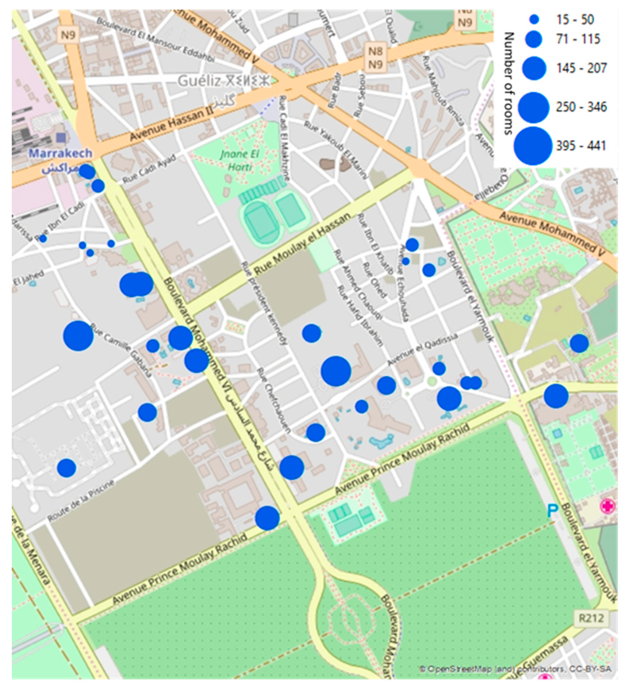
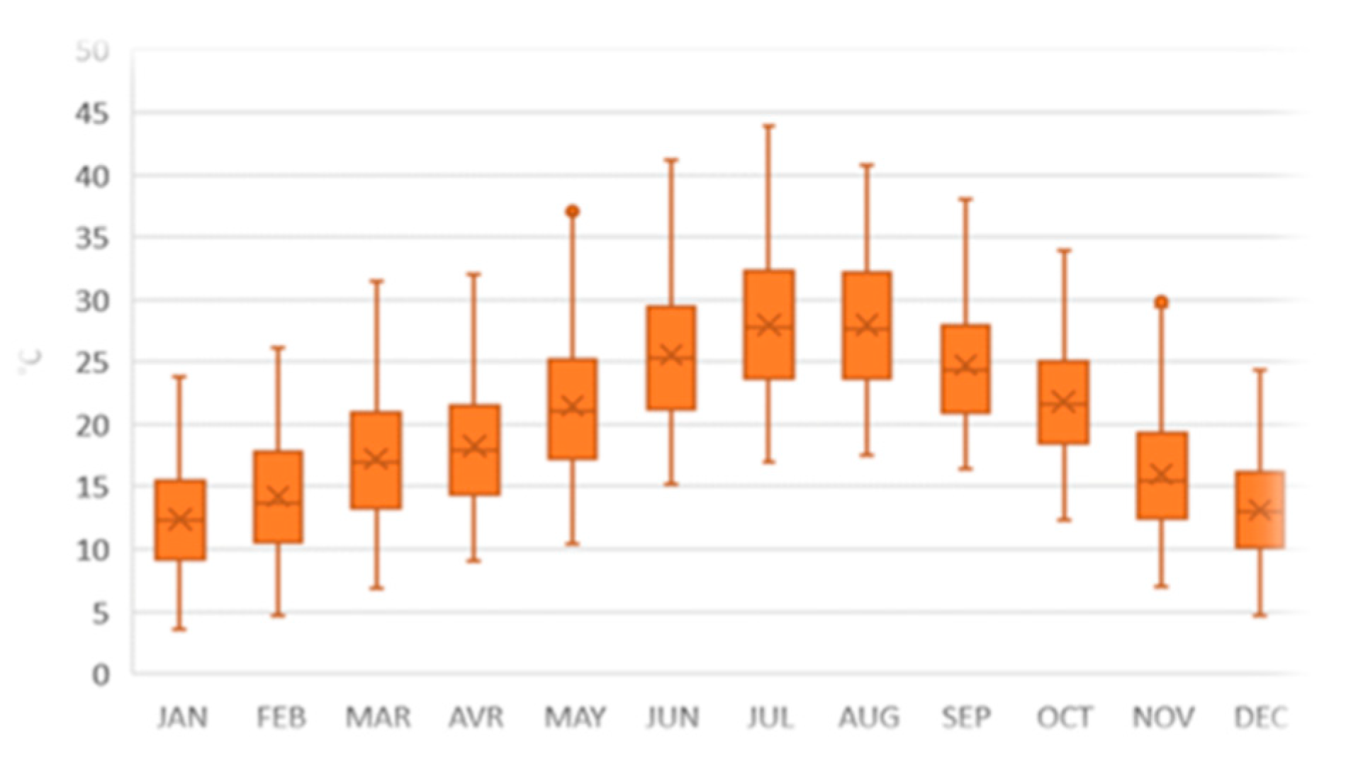
3. Case Study Description

The proposed methodology is employed in a feasibility study and the preliminarily design of a district cooling system the in city of Marrakech.

Marrakech is classified as BSh (hot semi-arid Steppe climate) under Köppen climate classification [25].

Marrakech climate data for a typical year are generated using the Meteonorm database (the standard periods are 1991–2010/1996–2015 for irradiation data and 2000–2009 for the other parameters).

In Figure 1 and Figure 2, the box and whisker graphs illustrate the hourly distribution of temperatures and humidity during each month.

It can be seen the temperature is above the water-freezing temperature all year long. The highest average temperature occurs during July. Relative humidity as an average is below 50% during the summer, which means a low need of dehumidification.

The total number of cooling degree days (CDD) and heating degree days (HDD) for Marrakech are 650 (base temperature 22 °C) and 606 (base temperature 18 °C).

In Marrakech, the cooling season is dominant. Space cooling is usually provided by means of electric air-conditioning equipment such as window units and split systems. Although not all residential buildings are equipped with air conditioning systems, the application of these systems has grown rapidly in the last years [26].

Selected Area for DC Network Implementation

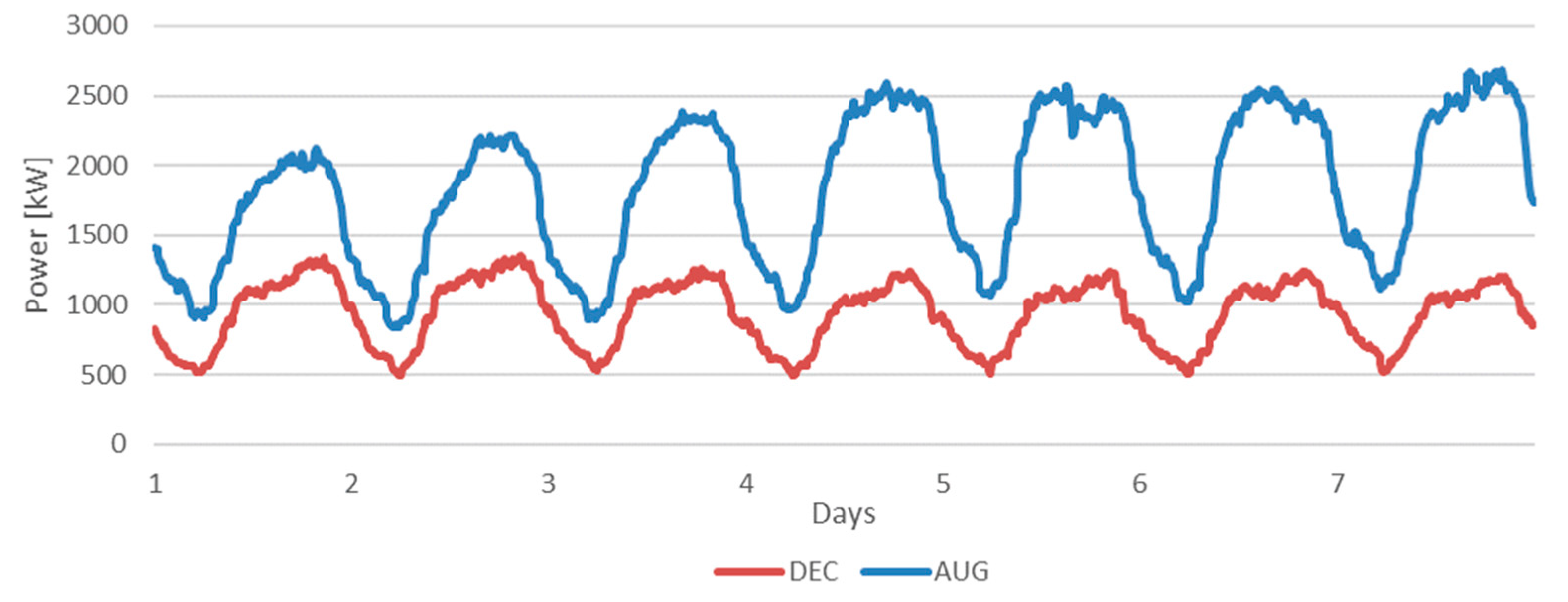
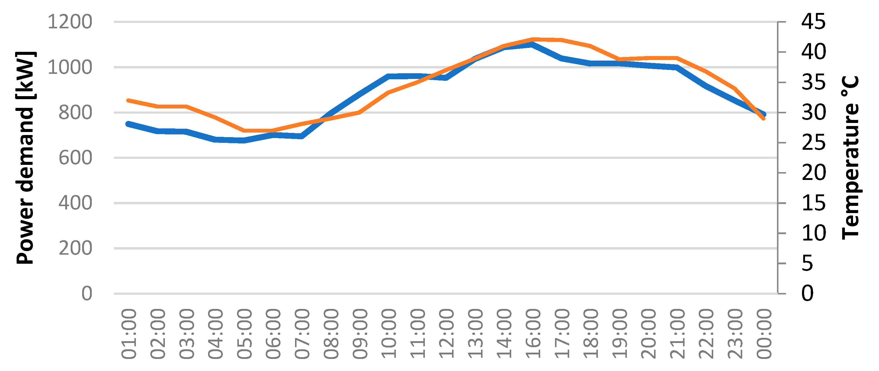
Marrakech is a city devoted to tourism with almost no industry and an office area that is not relevant. Regarding the air conditioning purposes, residential buildings usually use natural ventilation or split systems. Not all buildings benefit from air conditioning systems. However, almost all large buildings such as hotels, malls, hospitals, etc. provide space cooling and benefit from centralized cooling systems, e.g., chillers. In particular, hotel buildings, due to the high level of thermal comfort provided, are considered as one of the highest cooling demands among other types of buildings.

Two potential areas in Marrakech are namely Hivernage and Agdal. Most of the hotel buildings of the city are located in these two neighbourhoods. Since Hivernage hosts more hotels and its situated relatively close to the airport (which can be considered interesting for the future network extension), this neighbourhood is chosen as the area of study for the DC system. The area is situated in the north of Marrakech; in Figure 3, the location of the hotels in the district and room numbers (as an indication of the hotel size) are shown.

4. Results

In this section, the methodology is applied to the case study, and the results are presented. Therefore, the annual cooling energy need and its hourly profile are estimated.

District Cooling Demand and Profile Estimation

For the estimation of the cooling demand, a field survey has been performed. The monthly electricity consumption of hotels has been provided by the local utility provider.

In Figure 4, the sum of the monthly electricity consumption for a wide group of hotels in the area is illustrated for four years from 2014 to 2017 (December 2017 is not available). It can be seen clearly that peak electricity consumption occurs during August, and the lowest consumption occurs during March in all four years. Peak consumption (approximately 12,000 MWh in 2016 and 2017, and 11,000 MWh in other two years) is mainly due to the high electricity demand for cooling during the summer. On the other hand, low consumption during March is due to low or almost zero thermal needs (due to moderate outdoor temperature most of the time, passive strategies such as natural ventilation can bring the required thermal comfort). Although the number of bills varies each year, the minimum electricity consumption each year during March remains almost constant and equal to approximately 6000 MWh. Therefore, March can represent the month in which regardless of the occupancy rate and climatic conditions, the monthly electricity consumption is almost constant. Therefore, March is identified as the neutral month.

The decreasing consumption trend during June and July is probably due to the Ramadan period, as also confirmed by interviews with hotel administrators. When the occupancy rate drops sharply, some hotel sections would be closed, which results in lower consumption. Although the occupancy rate decreases dramatically during Ramadan, the electricity consumption during the Ramadan period is still more than the neutral month (when the occupancy rate is higher than Ramadan). This somehow is a confirmation of what stated in Section 1.2; that is, the electricity used for cooling in a high-standard hotel, as the case of Hivernage, is not strongly affected by occupancy rate.

The Ramadan period during each year is reported in

Table 2. Ramadan period from 2014 to 2017.

	2014	2015	2016	2017
Ramadan	28 June to 27 July	18 June to 17 July	6 June to 5 July	27 May to 25 June

.

To validate the result obtained, we have applied the methodology of the European Cooling Index (ECI) to perform a comparison [17]. We applied this methodology because of the lack of similar data for Morocco in the literature, and since the climate in Marrakech is similar to other European countries such as Spain and Italy [25], while comparison with other countries can be very uncertain [16].

The value calculated with the ECI index methodology is of the order of magnitude of 180 kWh/m²/year, while the value calculated with the proposed methodology is around 150 kWh/m²/year.

In addition, Jakubcionis and Carlsson [18] have estimated the European service sector space cooling potential through taking United States (US) consumption data as proxy. By employing this method for the case study, the obtained results (approximately 140 kWh/m²/year) are less than 7% different from the results obtained from the application of the proposed methodology.

Moreover, an estimation of the cooling energy demand of the existing hotels in the Marrakech climatic zone has been performed by Moroccan energy efficiency Agency (AMEE): the results obtained with our methodology are about 20% varying compared to AMEE estimation [27].

The building energy performance standard EN ISO 13790, for a single-building cooling demand estimation, considers a deviation of 50% to 150% from the actual results acceptable, due to several usually uncertain parameters [28]. Considering that the proposed methodology is for cooling demand estimation at the district level and for the planning phase of DCs, the deviations are in an acceptable range.

In addition, the hourly electricity consumption profile of available hotels shows a consumption pattern that strictly follows the variation of the external temperature. As an example, the hourly electricity consumption of one hotel in Marrakech in the first week of August 2017 and in the first week of December 2017 is shown in Figure 5. This behaviour confirms the hypothesis of considering the external conditions as the main influencing factor of the cooling demand for our case, although the method does not consider other influencing factors, as described in [29,30]. The peak in the winter is much lower than that in the summer, and occurs during the night-time, while in the summer, the peak occurs close to midday.

In Figure 6, the variation of the electric power of a hotel building is compared with the variation of hourly outdoor temperature during a typical summer day in Marrakech. It can be clearly seen that the hourly electricity consumption and outdoor temperature follow a very similar trend. However, the peak electric power occurs at around 15:00 when the solar irradiation is more intense, while the highest outdoor temperature is at around 17:00. When the outdoor temperature is near the thermal comfort range, the variation of electric power seems to be negligible. These behaviours affirm the dependence of the cooling power on the difference between the sol–air temperature and the set-point temperature.

Finally, based on surveys and climate analysis, it has been highlighted that most of the hotel buildings in Marrakech do not provide dehumidification, due to an acceptable level of relative humidity during the summer. Therefore, the effect of dry-bulb temperature and solar irradiation is considered to have the most influence on the overall cooling energy need of the district.

In order to consider the effect of solar irradiation on different orientations and slopes, the average of solar irradiation on a horizontal surface (representing the roof), and four orientations of vertical surfaces (representing the walls) is calculated. Since the four surfaces are vertical and this term would be zero, for simplification, it is considered negligible.

The surface solar absorbance and heat transfer coefficient terms for light colour horizontal and vertical surfaces are considered equal to 0.75 and 25 W/m²K, respectively [24].

Therefore, by considering an indoor set-point temperature equal to 22 °C (reported by hotels), the hourly load profile is estimated by distributing the total yearly demand (i.e., around 25 GWh/year) hourly and proportional to the difference of the sol–air temperature and indoor set-point temperature during the cooling season (the cooling season could be longer in Marrakech, however, to stay on the safe side and not overestimate the cooling load, it is considered from April to September), see Figure 7.

5. Preliminary Design and Evaluation Framework for DC Planning

In the following, a step-by-step framework aims to facilitate the preliminary design and feasibility evaluation of a district cooling system during the planning phase.

5.1. Preliminary Design of DC

Having the hourly cooling demand of the area under study, delta T (∆T) is usually the next key parameter to be assigned. Delta T is the difference between the supply and return temperatures:

$$\Delta T=T_{return}-T_{supply}$$

(14)

Basic theoretical thermodynamics shows that changes in temperature of the hot and cold sides of the chiller affects the coefficient of performance (COP) of the system. Therefore, after defining the temperatures, the average seasonal COP of the system should also be estimated using the selected chiller’s technical sheet information or more detailed correlations such as [31].

Having the hourly cooling energy need q, the specific heat C_p of the heat carrier fluid (e.g., water), and the design ∆T, the required flow rate $\dot{m}$ in each time step can be calculated as follows in Equation (15):

$$\dot{m}=\frac{q}{C_P\Delta T}$$

(15)

Then, the maximum piping diameter d in m for each piping branch can be calculated using Equation (16):

$$d=\sqrt{\frac{4\dot{V}}{\pi v}}$$

(16)

where $\dot{V}$ in m³/s is the maximum volumetric flow rate in each branch, which can be obtained by assuming the power to be proportional to the piping branches’ length, and v in m/s is the maximum allowable flow velocity (usually is considered between 2.5 m/s to 3 m/s depending on the future expansion of the district cooling network [32]).

To size the pump, the required pump head $\Delta p_{pump}$ in Pa should overcome the pressure drops in supply and return lines $\Delta p_{piping}$ plus the minimum pressure differential system (usually six meters of water) at the critical node of the system $\Delta p_{min}$, i.e., the point with the lowest pressure. Then, the electrical power of pump can be calculated by Equation (19):

$$\Delta p_{piping}=-\frac{8fL}{d^5{\pi }^2\rho }·{\dot{m}}^2$$

(17)

$$\Delta p_{pump}=\Delta p_{piping}+\Delta p_{min}$$

(18)

$$P_{el}=\frac{\Delta p_{pump}}{{\eta }_{pump}}·\dot{V}$$

(19)

where L is the length of the piping branches in m, $\rho$ is the density of the heat carrier in pipes in kg/m³, and ${\eta }_{pump}$ is the pump efficiency. $f$ is the friction factor in pipes that can be calculated using the Darcy–Weisbach formula, as shown in Equation (20):

$$f=8{\left[{\left(\frac{8}{R{e}_{D_h}}\right)}^{12}+\frac{1}{{\left(A+B\right)}^{1.5}})\right]}^{\frac{1}{12}}$$

(20)

where Re, A, and B can be calculated as follows:

$$A={\left[2.457ln\frac{1}{{(7/R{e}_{D_h})}^{0.9}+\left(0.27\epsilon /D_h\right)}\right]}^{16}$$

(21)

$$B={\left(\frac{37530}{R{e}_{D_h}}\right)}^{16}$$

(22)

$$Re=\frac{\rho VD}{\mu }$$

(23)

Then, the pumping electricity consumption can be estimated by employing equivalent full-load hours (EFLH). EFLH, which is measured in hours, is the ratio of annual cooling energy to the peak demand (24):

$$EFLH=\frac{Q_{cooling}}{q_{max}}$$

(24)

where Q_cooling is the annual cooling energy consumption in kWh/year, and q_max is the peak hourly consumption in kW.

The heat gains of the distribution system in W can be estimated using Equation (25). Then, by multiplying it with the total cooling season hours, the total energy gains in the piping system can be calculated:

$$q_L=\frac{T_f-T_s}{R_s+R_p}·L$$

(25)

where T_f is the average of the supply and return temperatures of fluid, T_s the average temperature of the soil (which can be calculated or can be approximately considered equal to the average annual air temperature), and L is the piping length. The thermal resistance of the soil $R_s$ in mK/W and thermal resistance of piping $R_p$ in mK/W should be calculated using Equations (26) and (27):

$$R_s=\frac{\ln (\frac{2b}{r_o})}{2\pi k_s}$$

(26)

$$R_p=\frac{\ln (\frac{r_o}{r_i})}{2\pi k_p}$$

(27)

where k_s and k_p are the thermal conductivity of the soil and pipe (including the insulation layer if present) respectively in W/mK, b is the depth at which pipes are buried in m, and r_i and r_o are the internal and external diameters of the pipe in m, respectively.

Sensitivity analysis in the next phases of the planning should be performed for the optimised design of components.

Considering the surveys performed, most of the existing individual systems in Marrakech hotels work between 7–12 °C. Therefore, starting from the customers’ required supply temperature and considering at least a 1 °C temperature offset in the heat exchanger and an 0.5 °C increase in temperature due to thermal gains in piping (0.05–0.1 °C/km), the supply temperature in a DC generation plant should be around 5.5 °C. Using the same procedure results in 11.5 °C for the return temperature. Thus, the average delta T of DCS is equal to 6 °C.

In the absence of industrial excess heat and sources of “free cooling” such as underground water in rivers and lakes, as well a gas distribution network, air-cooled or water-cooled chillers result in appropriate options for providing chilled water.

The two alternatives and the existing individual hotel building generation plants are compared in

Table 3. Comparison of possible generation plants’ COP.

Scenario	Heat Rejection Component	Average Seasonal COP
Individual air-cooled	Dry cooler	2.4
DC air-cooled	Dry cooler	3.4
DC water-cooled	Evaporative cooler (cooling tower)	5.1
	Treated greywater	3.8

according to their COP.

The maximum allowable velocity in a pipe is usually between 2.5–3.0 m/s [32]. Taking into account the potential increase in the number of buildings connected to the DC network and expansion plans in the future, the maximum allowable velocity is taken with an offset lower than the maximum allowable velocity of 2.8 m/s.

The piping system material is considered high-density polyurethane (HDPE), which brings advantages in terms of thermal performance, leakage, weight, and flexibility. A typical HDPE pipe’s conductivity is 0.4 W/mK, and the frictional losses are calculated for each main piping branch.

The soil temperature is estimated using the software TRNSYS®. The average temperature during the summer (from April to September) at one-meter depth (which is estimated as the buried piping depth) is equal to about 26 °C. Therefore, the thermal gains for each branch of the distribution system are calculated.

The volume of chilled water storage at 5.5 °C is selected to be equal to 3500 m³, which can answer about four hours of the average cooling demand.

Therefore, these four hours of thermal energy storage (TES) coverage are considered to occur during the peak electricity tariff hours, which can reduce the average electricity tariff of the DC system.

The main parameters’ metrics within the Marrakech DC system are summarized in Figure 8.

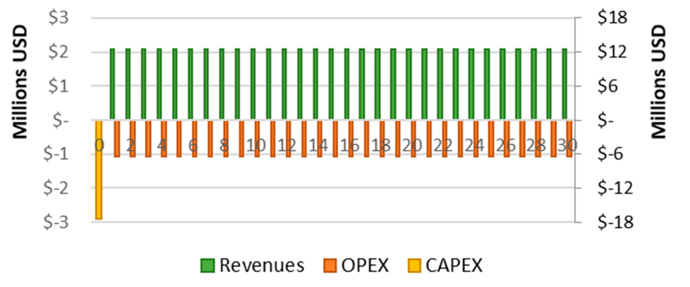
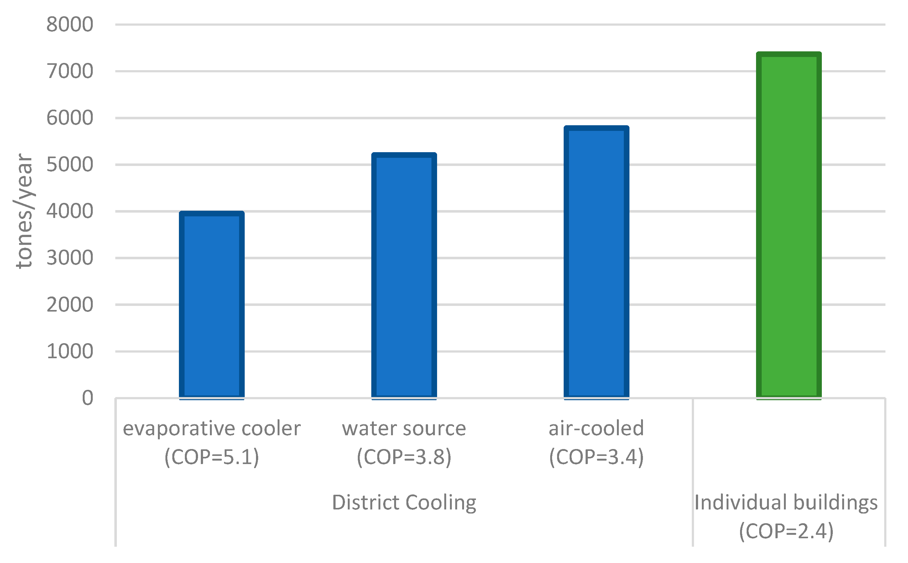
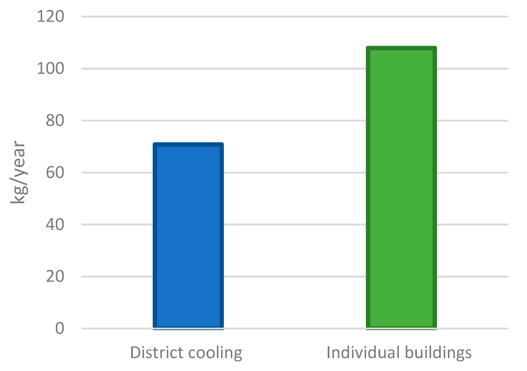
5.2. Economic and Environmental Evaluations.

Four main economic indicators can be considered to evaluate the economic feasibility of the DC project, namely net present value (NPV), internal rate of return (IRR), payback time (PBT), and return on investment (RoI).

Net present value (NPV) is the current value of the expected future cash flows (cumulative costs and incomes) over the lifetime of the system, as shown in Equation (28):

$$NPV={\displaystyle \sum }_{i=1}^n\frac{C{F}_i}{{\left(1+r\right)}^i}$$

(28)

where i is the year, r is the real discount rate (interest rate minus inflation rate), and CF_i in $/year is the cash flow in year i. The CF_i of each year is the summation of all expenditures—such as capital expenditures (CAPEX) and operational expenditures (OPEX)—and all the revenues—such as the cold purchase and subsidies—of that year.

CAPEX are the investments needed in the first years of the DC system, and include:

• all costs regarding the cooling plant such as building construction, chillers, cooling towers, and controls,
• distribution systems such as excavation, backfill, piping, pumps, and valves,
• thermal energy storage (TES),
• substations, and
• other costs such as cost of land, design, etc.

When actual costs are not available, they can be expressed based on the $/kWh cooling capacity that can be found in the literature. OPEX are the project running costs during the entire lifetime of the DC system (since the operation of system is only known under actual working conditions, operation and maintenance (O&M) costs are usually considered as a percentage of CAPEX on an annual basis). These costs depend on the system operation and equipment lifetimes. OPEX include:

• Operation and maintenance (O&M) such as maintenance, repairing and replacing the components, labour for operation, etc.,
• energy and power charge costs,
• water consumption costs,
• rent, and
• other costs such as administrative costs, insurance, etc.

Revenues are cold purchased to the customers, or include possible incentives and services.

The internal rate of return (IRR) is the discount rate that makes the NPV of all the cash flows equal to zero at the end of a specific year i (e.g., lifetime of the project). The payback time (PBT) is the year that the NPV would be equal to zero.

$$0={\displaystyle \sum }_{i=1}^n\frac{C{F}_i}{{\left(1+IRR\right)}^i}$$

(29)

Return on investment (RoI) demonstrates the efficiency of the investment by comparing the ratio present value of the gains (at the end of system lifetime) to investment (CAPEX):

$$RoI=\frac{NPV}{CAPEX}$$

(30)

Of course, for a DC system, the economics of the project is extremely site-specific, and depends on various local parameters. Thus, for the next stage of the project, more detailed economic input is required for the above-mentioned calculations.

The main influencing input parameters are divided into categories and quantified for both DC and individual buildings. Thus, capital expenditures (CAPEX), operating expenditures (OPEX), and revenues are estimated (in all calculations, value-added tax (VAT) is excluded).

Although some components may have a longer lifespan, the overall lifetime of a DC system in Marrakech is estimated to be 30 years.

The estimated price list is based on the local consultant survey, similar projects, the literature, and international consultants, as summarized in

Table A1. Capital expenditures (CAPEX) price list. TES: thermal energy storage.

Item		Price	Unit	Note
DC system	Generation plant	600,000	USD/MW	The price includes all costs related to and located in DC generation plant such as design, building construction, chillers, refrigerant, cooling towers, primary and secondary pumps, control system, electrical transformers, and water supply equipment for cooling towers.
	Distribution	300	USD/m	Per meter of pipe. The price includes excavation, backfill, surface restoration, high-density polyurethane (HDPE) pipes, valves, joint connection, and installation fee.
	TES	5000	USD/MWh	Chilled water tank with heat exchangers and pumps.
	Substations	25,000	USD/MW	All costs from main pipe to end-users boundary (heat exchanger) including small pipes, metering, valves, etc.
	Land	600	USD/m2	The estimated cost of land (more than 1000 m2) in the Hivernage area.
Standalone cooling systems (individual hotels cooling system)	Central cooling plant	620,000	USD/MW	The price includes chillers, pumps, cooling towers, control system, electrical/water supply equipment, valves, piping inside the mechanic room, and installation fee.

and

Table A2. Operating expenditures (OPEX) price list.

Item		Price	Unit	Note
DC system	Operations and maintenance (O&M)	2%	CAPEX/year	It includes all cost related to the maintenance of all the DC plant equipment and components including repair, replace, refill of refrigerant, and the labour fee.
	Electricity consumption	81	USD/MWh
	Power capacity charge	44,967	USD/MW
	Water consumption	0.6	USD/m3
	Land rent	4%	Land value/year	Land is assumed to be rented. The rent is estimated as a percentage of the land value.
Standalone cooling systems (individual hotels cooling system)	O&M	4%	CAPEX/year	The price includes all costs related to O&M of individual buildings central generation plant such as repair, replace, refill of refrigerant, and the labour fee. This cost exclude the O&M of the internal distribution system, since they would be still present in the case of a DC system as well.
	Electricity consumption	118	USD/MWh	It is calculated as the average hotel bill.
	Power capacity charge	44,967	USD/MW	The cooling-related power for individual buildings is higher than that of a DC (25% of power is related to cooling, and this is reduced based on COP ratios.

in Appendix A.

The investment cost for an individual hotel’s cooling plant is also estimated, including their O&M cost calculation. Usually, the cooling plant investment cost per cooling power in a DC system is lower than standalone cooling systems due to the advantages obtained in the economy of scale in a DC system.

The cost of electricity consumption and power capacity charge are calculated based on the total electricity used in all the DC components and the maximum electric power of the system. Since the electricity tariff changes during different hours of the day, the weighted average of electricity tariffs during a day is considered as the fixed electricity tariff. When thermal storage is present, it is considered to be employed during the peak electricity tariff to reduce the fixed electricity price and decrease the energy costs. As well, for water consumption, the associated cost due to leakages and/or the water used in cooling towers is calculated. In Marrakech, the electricity tariff for medium-voltage consumers is the same regardless of the size of the consumers. Thus, the electricity price for centralized chillers is the same as that for the individual small chillers. Nevertheless, one of the advantages of the DC system is that through eliminating the electricity consumption due to cooling, hotels connected to DC can decrease the fraction of the electricity bill due to the power capacity installed. In addition to that, due to contemporaneity effects, the peak demand of a DC system is anyway lower than the sum of the peak demand of single consumers.

Regarding the single hotels, it is assumed that individual cooling systems’ O&M costs include only the central cooling plant, and not their distribution system. This assumption is because the O&M of an internal distribution system in hotel buildings also still exists in the case of them being connected to a DC network.

The only revenue is from costumers’ cold purchase, and no other charge is applied. In order to figure out the cold tariff, expenditures (CAPEX and OPEX) for space cooling purposes, and accordingly, an approximation of the cost of cooling per each unit of energy is estimated for individual hotel buildings.

The estimated amount of outgoing cash, i.e., CAPEX (on the right vertical axis) and OPEX, and the incoming cash (on the left vertical axis), i.e., revenues for each year and during the lifetime of DC system are illustrated in Figure 9. The outgoing cash is considered negative, and the incoming cash is considered positive.

The real discount rate in the calculation of present values is assumed to be 2.5%. This value represents the public and private joint venture (50%–50%).

The summary of economic indicators for the Marrakech DC system is reported in

Table 4. Marrakech DC economic indicators. PBT: Payback Time, IRR: internal rate of return, ROI: return on investment.

Net Present Value (USD)	PBT (years)	IRR (30 years)	ROI
3,822,353	23	4.1%	21.9%

.

To account for CO₂ emissions, the electricity consumption should be converted into carbon dioxide equivalent (CO₂ emissions and other greenhouse gases than CO₂ in the production of electricity can be also considered) by using the corresponding emission factor.

A significant reduction in the consumption of environmentally damaging refrigerants such as chlorofluorocarbons (CFCs) and hydrofluorocarbons (HFCs) can be achieved by DC. To estimate the reduction in refrigerant emissions, the volume of leakages in chillers during the lifetime is usually reported as a percentage of the maximum cooling power of the chillers.

The water savings also can be estimated based on the heat rejection capacity requirement of chillers.

It should be added that the benefits due to employing thermal energy storage (TES) include reducing the chiller maximum design capacity and the average electricity tariff (shifting the generation from the peak tariff period to an off-peak tariff). In addition, employing the renewable energy sources (RES) will result in lower CO₂ emissions, and thus usually a lower electricity tariff.

Since the only energy source in both individual cooling systems and a DC system is electricity, the electricity consumption is converted into carbon dioxide equivalent (CO₂ emissions and other greenhouse gases than CO₂ in the production of electricity are also considered) by using an emission factor of 707.8 g/kWh_elec (for the year 2014) [27]. Therefore, the COP of each system is the main parameter in the CO₂ emissions variation in each system.

Figure 10 clearly shows that in terms of CO₂ emissions and electricity consumption, the district cooling system provides approximately 21% to 46% savings in comparison with individual systems.

The refrigerant emissions (R14a) for both the DC system (water-cooled chillers) and individual buildings (air-cooled) are estimated as well. Figure 11 shows that by employing the DC system, the refrigerant emissions can be reduced approximately by 34% per year in comparison with refrigerant leakages in individual cooling systems.

6. Discussion and Conclusions

District cooling represents an important solution to decrease the greenhouse gas emissions related to space cooling, in particular in urban contexts. However, its diffusion is still limited, and many difficulties arise in correctly sizing a DC plant due to the variability and amount of data required. In this paper, a measurement-based method to reduce these difficulties has been presented, which is based on easily retrievable data such as electricity bills. The proposed methodology can facilitate the demand estimation and therefore the planning of the DCSs.

The approach relies on the relationship between cooling demand and the seasonal variation of building electricity bills. The novelty of the study is that a typical approach used for district heating, such as the use of fuel consumption to estimate the demand, is adopted for district cooling. Since the amount of data required for single buildings within a district represent a challenging barrier, this approach can be effective in cases where the access to building envelope data is difficult.

An important hypothesis at the base of the methodology is that outdoor weather is considered to be the main influencing factor affecting the cooling demand profile. This assumption is in line with the scientific literature analysed and supported by the available field data, as shown in Section 4.

However, the scientific literature also demonstrates that this hypothesis is more applicable in cases where the district is constituted mainly by tertiary and commercial buildings, as done in this study. Indeed, the methodology is applied to the case study of a DC network project in the Hivernage district of Marrakech that includes more than 40 hotels. The results obtained are validated by comparison with other methodologies, as described in Section 4.

This assumption certainly represents a limit of the methodology, since the occupancy rate in residential buildings affects the cooling demand profile. Therefore, the application of the methodology to residential districts requires further analysis.

Finally, concerning the case study, although resulting in a positive RoI, the economic assessment suggests a deeper local analysis of component cost and tariff incentives, since the payback time of 23 years might only be attractive for public institutions, and not private investments. Indeed, the environmental evaluations demonstrate all the advantages of investing in a district cooling system, including peak electricity reduction, higher efficiency, and greenhouse gas emission reduction compared to the individual solutions. Hence, this result confirms that that the economic feasibility of DC systems is extremely context-related. The seasonal demand requires maximizing the investment return over an operating time that is much lower than the plant lifetime. Therefore, the higher the cooling season, the higher the time to scale the revenues, and the lower the cost for users that are more attracted to connect to the DC network.

In the future research works, by a more inclusive set of measured data such as hourly solar radiation and hourly cooling energy use of different typologies of commercial buildings, it is possible to extend the proposed methodology to other building types and estimate the related level of uncertainty. In addition, the focus can go beyond the cooling energy need and the proposed methodology can be employed in other climatic zones.

References

1. Rao, L.; Chittum, A.; King, M.; Yoon, T. Governance Models and Strategic Decision-Making Processes for Deploying Thermal Grids; International Energy Agency, 2017. Available online: https://www.districtenergy.org/HigherLogic/System/DownloadDocumentFile.ashx?DocumentFileKey=e24e4c4e-3cd8-825e-d1eb-518dc945632c&forceDialog=0 (accessed on 19 February 2018).
2. UNEP District Energy in Cities. Unlocking the Potential of Energy Efficiency and Renewable Energy. United Nations Environment, 2015. Available online: https://wedocs.unep.org/bitstream/handle/20.500.11822/9317/-District_energy_in_cities_unlocking_the_potential_of_energy_efficiency_and_renewable_ene.pdf?sequence=2&amp%3BisAllowed= (accessed on 19 February 2018).
3. The Future of Cooling. Opportunities for Energy-Efficient Air Conditioning; International Energy Agency, 2018; p. 90. Available online: https://webstore.iea.org/the-future-of-cooling (accessed on 01 December 2018).
4. Rismanchi, B. District energy network (DEN), current global status and future development. Renew. Sustain. Energy Rev. 2017, 75, 571–579. [Google Scholar] [CrossRef]
5. Rescue District Cooling and the Customers’ Alternative Costs (RESCUE WP2). 2014, p. 42. Available online: http://www.rescue-project.eu/ (accessed on 6 February 2018).
6. Ashrae District Cooling Guide; ASHRAE: Atlanta, GA, USA, 2013; ISBN 9781936504428, 9781936504435.
7. Resque Best Practice Examples of District Cooling Systems. 2015. Available online: http://www.rescue-project.eu/ (accessed on 16 January 2018).
8. Frayssinet, L.; Merlier, L.; Kuznik, F.; Hubert, J.L.; Milliez, M.; Roux, J.J. Modeling the heating and cooling energy demand of urban buildings at city scale. Renew. Sustain. Energy Rev. 2018, 81, 2318–2327. [Google Scholar] [CrossRef]
9. Zhao, H.X.; Magoulès, F. A review on the prediction of building energy consumption. Renew. Sustain. Energy Rev. 2012, 16, 3586–3592. [Google Scholar] [CrossRef]
10. Gustafsson, M.S.; Myhren, J.A.; Dotzauer, E. Mapping of Heat and Electricity Consumption in a Medium Size Municipality in Sweden. Energy Procedia 2017, 105, 1434–1439. [Google Scholar] [CrossRef]
11. Swing Gustafsson, M.; Myhren, J.A.; Dotzauer, E. Potential for district heating to lower peak electricity demand in a medium-size municipality in Sweden. J. Clean. Prod. 2018, 186, 1–9. [Google Scholar] [CrossRef]
12. Woods, P. Heat Networks: Code of Practice for the UK—Raising Standards for Heat Supply; CIBSE: London, UK, 2015; ISBN 9781906846626. [Google Scholar]
13. Commonwealth Energy Efficiency Opportunities in the Hotel Industry Sector, 2002; 1–43.
14. Priyadarsini, R.; Xuchao, W.; Eang, L.S. A study on energy performance of hotel buildings in Singapore. Energy Build. 2009, 41, 1319–1324. [Google Scholar] [CrossRef]
15. Tang, M.; Fu, X.; Cao, H.; Shen, Y.; Deng, H.; Wu, G. Energy performance of hotel buildings in Lijiang, China. Sustainability 2016, 8, 780. [Google Scholar] [CrossRef]
16. Wang, J.C. A study on the energy performance of hotel buildings in Taiwan. Energy Build. 2012, 49, 268–275. [Google Scholar] [CrossRef]
17. Dalin, P.; Nilsson, J.; Rubenhag, A. EcoHeatCool WP2: The European Cold Market. Work Packag. Deliv. Ecohaetcool EU Proj. 2005, p. 45. Available online: https://www.euroheat.org/wp-content/uploads/2016/02/Ecoheatcool_WP2_Web.pdf (accessed on 3 December 2018).
18. Jakubcionis, M.; Carlsson, J. Estimation of European Union service sector space cooling potential. Energy Policy 2018, 113, 223–231. [Google Scholar] [CrossRef]
19. DeRoos, J. Planning and programming a hotel. Cornell University School of Hospitality Administration The Scholarly Commons. 2011, pp. 321–332. Available online: http://scholarship.sha.cornell.edu/articles/310 (accessed on 11 January 2018).
20. Gang, W.; Augenbroe, G.; Wang, S.; Fan, C.; Xiao, F. An uncertainty-based design optimization method for district cooling systems. Energy 2016, 102, 516–527. [Google Scholar] [CrossRef]
21. Kohler, M.; Blond, N.; Clappier, A. A city scale degree-day method to assess building space heating energy demands in Strasbourg Eurometropolis (France). Appl. Energy 2016, 184, 40–54. [Google Scholar] [CrossRef]
22. Berger, M.; Worlitschek, J. A novel approach for estimating residential space heating demand. Energy 2018, 159, 294–301. [Google Scholar] [CrossRef]
23. Ciulla, G.; Lo Brano, V.; D’Amico, A. Numerical Assessment of Heating Energy Demand for Office Buildings in Italy. Energy Procedia 2016, 101, 224–231. [Google Scholar] [CrossRef]
24. ASHRAE. ASHRAE Fundamentals 2009; ASHRAE: Atlanta, GA, USA, 2009; ISBN 6785392187. [Google Scholar]
25. World Maps Of Köppen-Geiger Climate Classification. Available online: http://koeppen-geiger.vu-wien.ac.at/ (accessed on 6 May 2018).
26. Mansour, S.; Castel, V. Morocco 2014: Energy Policies Beyond IEA Countries; International Energy Agency Publications. 2014, p. 13. Available online: https://www.iea.org/publications/freepublications/publication/Morocco2014.pdf (accessed on 16 November 2018).
27. Règlement Thermique de Construction au Maroc, Moroccan Energy Efficiency Agency. 2014. Available online: http://architectesmeknestafilalet.ma/documentation_telechargements/Efficacit%C3%A9%20energetique/Reglement_thermique_de_construction_au_Maroc_-_Version_simplifiee.pdf (accessed on 6 June 2018).
28. EN ISO 13790. Energy Performance of Buildings. Calculation of Energy Use for Space Heating and Cooling; International Standard Association. 2008, p. 172. Available online: https://www.iso.org/standard/41974.html (accessed on 5 February 2018).
29. Bruno, R.; Arcuri, N.; Carpino, C. Cooling Energy Needs in Non-Residential Buildings Located in Mediterranean Area: A Revision of the Quasi-Steady Procedure. In Proceedings of the Third Building Simulation Applications Conference, Bozen, Italy, 8–10 February 2017. [Google Scholar]
30. Romani, Z.; Draoui, A.; Allard, F. Metamodeling the heating and cooling energy needs and simultaneous building envelope optimization for low energy building design in Morocco. Energy Build. 2015, 102, 139–148. [Google Scholar] [CrossRef]
31. Hydeman, M.; Gillespie, K.L.; Dexter, A.L. Tools and techniques to calibrate electric chiller component models. ASHRAE Trans. 2002, 108 Pt 1, 733–741. [Google Scholar]
32. Skagestad, B.; Mildenstein, P. District Heating and Cooling Connection Handbook; Netherlands Agency for Energy and the Environment: Dutch, The Netherlands, 1999; ISBN 905748 0263. [Google Scholar]
Figure 1. Monthly temperature distribution in Marrakech.
Energies 12 00944 g001
Figure 2. Monthly humidity distribution in Marrakech.
Energies 12 00944 g002
Figure 3. Hotels location in Hivernage and their number of rooms.
Energies 12 00944 g003
Figure 4. Sum of monthly electricity consumption of Marrakech hotels from 2014 to 2017. “n” shows the number of considered hotels in each year.
Energies 12 00944 g004
Figure 5. Hourly electricity consumption of a hotel building in Marrakech during a typical week in summer and a typical week in winter.
Energies 12 00944 g005
Figure 6. Electric power variations (thick blue line: right vertical axis) of a hotel building in Marrakech and outdoor temperature (thin orange line: left vertical axis) during a typical summer day.
Energies 12 00944 g006
Figure 7. Hourly cooling energy need distribution based on the sol–air temperature method.
Energies 12 00944 g007
Figure 8. DC system main parameters metrics.
Energies 12 00944 g008
Figure 9. Cash flow of DC system over its lifespan.
Energies 12 00944 g009
Figure 10. Annual equivalent CO2 emissions of generation plant alternatives.
Energies 12 00944 g010
Figure 11. Annual refrigerant emissions.
Energies 12 00944 g011