Optimal Sizing of Storage Elements for a Vehicle Based on Fuel Cells, Supercapacitors, and Batteries

Abstract

To achieve a vehicle-efficient energy management system, an architecture composed of a PEM fuel cell as the main energy source and a hybrid storage system based on battery banks and supercapacitors is proposed. This paper introduces a methodology for the optimal component sizing aiming at minimizing the total cost, achieving a cheaper system that can achieve the requirements of the speed profiles. The chosen vehicle is an urban transport bus, which must meet the Buenos Aires Driving Cycle, and the Manhattan Driving Cycle. The combination of batteries and supercapacitors allows a better response to the vehicle’s power demand, since it combines the high energy density of the batteries with the high power density of the supercapacitors, allowing the best absorption of energy coming from braking. In this way, we address the rapid changes in power without reducing the global efficiency of the system. Optimum use of storage systems and fuel cell is analyzed through dynamic programming.

1. Introduction

Today, one of the topics of interest in scientific research is the depletion of the planet’s natural resources. The energy that comes from fossil fuels such as coal and oil, among others, will be exhausted in the next future. Moreover, this type of energy produces environmental pollution and greenhouse gases, which are responsible for the biggest damage to the ozone layer. Energy consumption in the transport sector is known to be very large, around 29.5% of the total energy consumed [1]. In particular, vehicles are responsible for most of the energy consumed [2]. For this reason, environmental deterioration is one of the main causes of the development of energy management research in vehicles. Hybrid vehicles have been a step forward in this direction, and the advantages of hybridizing a system [3] can be summarized as:

• The vehicle can recover a fraction of the kinetic energy while braking (regenerative breaking)
• The main power source might be shut down during idle periods and low-load phases without compromising vehicle drivability
• The main power source can operate at high efficiency points independently of the vehicle trajectory.
• The main power source can be designed with a slightly lower capacity.

Articles like [4,5,6,7,8], use a battery as an auxiliary energy recovery system, while others as [9,10,11] use a supercapacitor for that purpose. Currently, there are combinations of both. Combining the energy density of the batteries with the power density of the supercapacitors increases fuel economy [12,13,14].

To replace combustion engines, other devices as fuel cells have been introduced [15,16,17]. According to [18], many previous studies have shown the effectiveness of fuel-cell-based vehicles. In addition, zero emissions and low noise generation make fuel cells a tempting energy converter for automotive powertrains. As an example of this, fuel cell-powered bus projects report that since 2011 there are approximately 100 of such buses distributed around the world.

Fuel cells have relatively high efficiency compared to internal combustion engines [19]. Ref. [20] contains a comparison between fuel cells and internal combustion engines in the transportation sector.

As shown in [21], the most common types of fuel cells on the market are proton exchange membrane fuel cells (PEMFC), direct methanol fuel cells, alkaline fuel cells, phosphoric acid fuel cells, molten carbonate fuel cells, solid oxide fuel cells, and microbial fuel cells. In this article, we will focus on the use of PEMFC. The sizing of the fuel cell systems and associated storage elements is a problem that must be treated with care, because its cost in the market is still high.

Usually, Fuel Cell Electrical Vehicles (FCEV) are composed of a fuel cell acting as main power source and an energy storage system (ESS). The ESS can contribute to improving the performance of an FCEV [22,23], reduce the FC size [24], improve the operating efficiency of the system [25,26], and extend the service life of the elements [27]. In FCEV, ESS is usually composed of a battery and/or supercapacitors. However, this hybridization involves a greater complexity of the system, which highlights the importance of energy management [28,29].

This paper proposes a methodology to obtain an optimal sizing of the ESS, composed of a battery and supercapacitors, in an urban transport FCEV. The combination of batteries and supercapacitors allows a better response to the vehicle’s power demand, since it combines the high energy density of the batteries with the high power density of the supercapacitors, allowing the best absorption of the energy coming from the braking. In this way, we address the rapid changes in power without reducing the global efficiency of the system.

Component optimal sizing aims to minimize the total cost while achieving the required performance. It is well-known that the vehicle performance depends a lot on the speed profile. For this reason, in this work two different urban driving profiles will be used as reference. In particular, the Buenos Aires Driving Cycle and the Manhattan Driving Cycle will be considered.

The proposed methodology will proceed as follows: firstly, the optimal energy evolution will be obtained using dynamic programming when following the considered speed profiles. This procedure will be repeated for different battery and supercapacitor sizes. Then, from the obtained results, optimal sizing will be determined.

The remainder of the paper is organized as follows: In Section 2, the vehicle architecture and the models of the components are described. In Section 3, the driving profiles are introduced and the theoretical amount of energy that can recover from regenerative braking is presented. Section 4 describes the ESS optimal sizing methodology based on dynamic programming. Section 5 presents the results of the sizing of the components in the considered vehicle with the proposed methodology. Finally, in Section 6, the main conclusions are drawn, introducing further research paths.

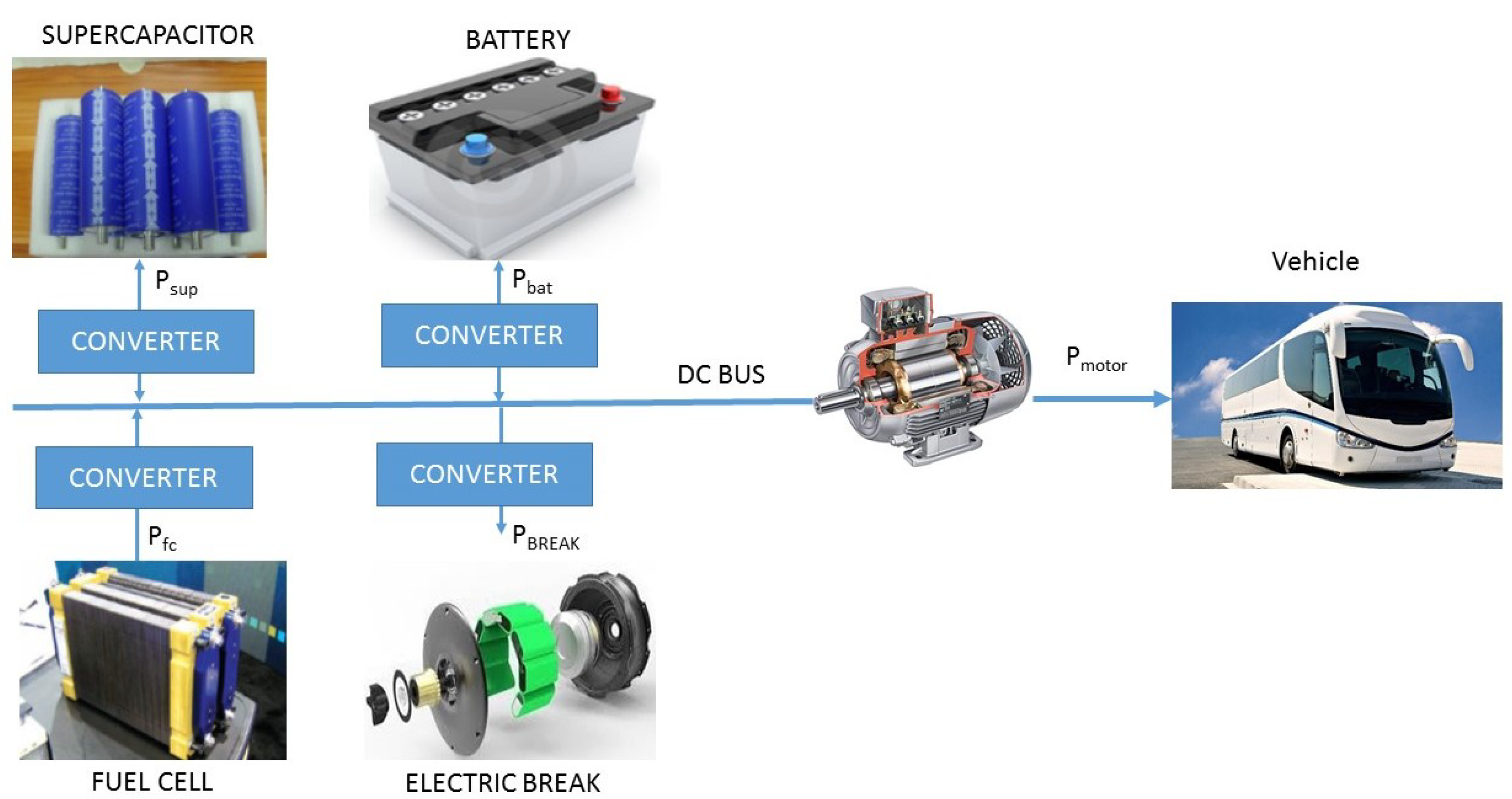
2. Vehicle Architecture

Vehicle architecture of HEV refers to the topological relationship and energy flow between its components [30,31]. The main configurations are the series, parallel, and series-parallel. Designing and selecting the architecture of an HEV’s is a critical procedure, as it influences future design, control, and optimization. As a first step, we will define the total power that the components of the vehicle’s propulsion system must deliver. The dynamics of the vehicle are based on the energetic balance of the forces that contribute to the movement of the vehicle, and those that oppose to it [32]. Then, we can express the mechanical power as a product of the forces and the speed of the vehicle. The inherent power of motion is deducted from the kinetic energy stored in it. The forces opposing the movement, are called dissipative forces, which are aerodynamic drag, frictional resistance to the ground and the resistance force due to the inclination of the road. Then, the mechanical power required to move the vehicle will be:

$$p_v={\displaystyle \frac{1}{2}}pv\left(s{c}_x\right)v^3+mgv{c}_{rr}+mgvsin\left(\alpha \right)+mv{\displaystyle \frac{dv}{dt}}$$

(1)

where m is the mass of the vehicle, $\alpha$ is the slope of the road, v is its speed, p is the air density, s is the front area of the vehicle, $c_x$ is the aerodynamic drag coefficient, g is gravity and $c_{rr}$ is the coefficient of rolling resistance. The parameters are based on a service bus, and are those shown in

Table 1. Parameters of the vehicle.

Name	Symbol	Value	Unit
Air density	p	1.2	kg/m${}^3$
Coefficient of resistance to movement	$c_{rro}$	0.008	s/u
Coefficient of resistance to movement	$c_{rrl}$	0.00012	s${}^2$/m${}^2$
Aerodynamic coefficient	$c_x$	0.65	s/u
Front area	s	8.06	m${}^2$
Total mass	m	14,000	kg
Gravity	g	9.8	m/s${}^2$

, being obtained from [33]. The total mass of the vehicle includes the mass of the chassis, the propulsion system, the components and the weight of the passengers. It should be noted that as the weight of the vehicle increases with the increase in the weight of its components and the number of occupants, more power is needed to reach the speed profile, because there are higher power peaks. Figure 1 shows the components of the propulsion system that will be part of the vehicle’s energy management. The main unidirectional source of energy is the fuel cell, which is connected to a DC converter. The storage elements (batteries and supercapacitor) are considered bidirectional, as they can deliver power to the movement, and at the same time, they can store the energy recovered from breaking. These elements are also associated with a DC converter. The speed profile can be placed as a power profile, and must be fulfilled by the sources. Then, the power balance can be expressed as:

$$p_v=p_{sup}+p_{bat}+p_{fc}+p_{break}$$

(2)

where $p_{sup}$ is the supercapacitor power, $p_{bat}$ is the battery power, $p_{fc}$ is the fuel cell power and $p_{break}$ is the power dissipated in the mechanical brake. As expressed in Equation (2), the sum of the powers of the elements must be equal to the mechanical power.

2.1. Battery Modelling

Electrochemical batteries are one of the key components in hybrid electric vehicles. Batteries, for specific energy management, will be characterized mainly in terms of power and energy. They are characterized by their nominal capacities, and by the state of charge (SOC), which describes the remaining energy stored in the battery, expressed as a percentage of its maximum capacity. Some desirable attributes of batteries for EV and HEV applications are high energy density and cycle life [34]. The energy density is a measure of the total amount of energy that a battery can store for a given mass. These elements can store considerable amounts of energy. Other features include long service life, low initial and replacement costs, high reliability, wide operating temperature range, and robustness. Battery operation is typically defined by a certain SOC window, whose limits are the minimum SOC during discharge and the maximum SOC during charging. Internal resistance is the factor that limits the battery’s charge and discharge efficiency. Resistance has different values under load and discharge conditions. Resistance and open-circuit voltage are non-linear functions of the battery SOC. A battery model can be derived from an equivalent circuit, where the battery is regarded as an open-circuit voltage source, in series with an internal resistor.

Depending on the amount of voltage/current, we connect a set of batteries, in series, in parallel, or a mixed connection series-parallel. For a series connection, the voltage supplied by the assembly is equal to the sum of the voltages. In parallel, the current increases as the sum of the number of batteries inserted. In both cases, the capacity always increases. According to [33], the equations for battery power charging and discharging should be taken into account as a function of SOC, where $p_{cb}$ is the charge power and $p_{db}$ is the discharge power

$$p_{cb}\left(k\right)=-{\displaystyle \frac{n_{bats}{u}_{cmax}^2-u_{oc}\left(k\right)u_{cmax}}{r_i}}{n}_{batp}$$

(3)

$$p_{db}\left(k\right)={\displaystyle \frac{-n_{bats}{u}_b{\left(k\right)}^2+u_{oc}\left(k\right)u_{cmin}}{r_i}}{n}_{batp}$$

(4)

where $u_b$ is the battery voltage, $u_{oc}$ is the battery open-circuit voltage, $r_i$ is the battery internal resistance, where $n_{batp}$ is the number of parallel cells and $n_{bats}$ is the number of serial cells and k is the discrete-time. The supercaps open-circuit voltage is a function of the battery charge. The total power of the battery will be the sum of $p_{db}$ and $p_{cb}$, and is called $p_{bat}^{*}$. The battery is also associated with a converter efficiency ${\delta }_{bat}$, which represents the losses in the converters and takes a value of 0.98. Then, we can define the total battery power $p_{bat}$ as shown.

$$p_{bat}\left(k\right)={\delta }_{bat}{p}_{bat}^{*}\left(k\right).$$

(5)

The considered battery is a prismatic Ni-MH one in a resin case. Battery parameters are shown in

Table 2. Battery parameters.

Parameter	Data
Manufacturer	PEVE
Shape	Prismatic
Case	Plastic
Cell capacity (Ah)	6.5
Cell voltage (V)	7.2
Specific energy (Wh/kg)	46
Specific power (W/kg)	1300
Mass (kg)	1.04
Operation temperature (°C)	−20 to 50
Cost (€/kg)	33.88

and taken from [35]:

2.2. Supercapacitor Model

Supercapacitor are energy accumulators. The specific power, or instantaneous power, that can deliver is greater than that of batteries, but their specific energy, or the amount of energy that can store is substantially less. In some cases, supercapacitors are used as primary ESSs, while in other cases, such as in this paper, they can be placed as a secondary storage system. This allows improvement of the performance of the main power system and the ESS. The equivalent circuit of supercapacitor consists of a capacitor that represents the capacitance and a series resistor that represents the ohmic losses in the electrodes and electrolyte [36].

In the model, we will redefine equations based on the capacitor state of energy (SOE). A detailed study of the process can be found in [34]. Then, the SOE is defined by:

$$SoE\left(k\right)={\displaystyle \frac{e_{sc}\left(k\right)}{e_{sc,t}}}$$

(6)

where $e_{sc,t}$ is the total storable energy and $e_{sc}$ is the instantaneous energy. Then, $e_{sc}$ is defined by:

$$e_{sc}\left(k\right)=\frac{1}{2}{c}_{sc}{q}_{sc}^2\left(k\right)$$

(7)

where $q_{sc}$ is the capacitor voltage expressed in (V), and $c_{sc}$ is the capacitance expressed in (F).

According to [34], the charging $p_{cs}$ and discharging power $p_{ds}$ is given by

$$p_{cs}\left(k\right)={\displaystyle \frac{n_{sc}{u}_{sc,max}(u_{sc}\left(k\right)-u_{sc,max})}{r_{sc}}}$$

(8)

$$p_{ds}\left(k\right)={\displaystyle \frac{n_{sc}{u}_{sc,min}(u_{sc}\left(k\right)-u_{sc,min})}{r_{sc}}}$$

(9)

where $n_{sc}$ is the number of elements, $u_{sc,max}$, and $u_{sc,min}$ are the supercapacitor voltage limits, $u_{sc}$ is the open-circuit voltage and $r_{sc}$ is the circuit resistance. A more detailed analysis and parameters can be found at [34]. The parameters used are from Maxwell 125 V Heavy transportation module, and are shown in

Table 3. Supercapacitor parameters.

Parameter	Data
Manufacturer	Maxwell Technologies
Packaging	Bulk
Cell capacitance (F)	3000
Rated Voltage (V)	125
Temperature (°C)	−40 to 65
Mass (kg)	1.3
Specific power (W/Kg)	1700
Specific energy (Wh/Kg)	2.3
$SO{E}_{max}$	1
$SO{E}_{min}$	0
Cost (€/Kg)	88.34

.

The power of the supercapacitor $p_{sup}^{*}$ is the sum of $p_{cs}$ and $p_{ds}$. The supercapacitor system is associated with an efficiency of the converter shown in Figure 1, ${\delta }_{sup}$, which represents the losses in the converters. In the current work, this parameter will take a value of 0.95. Then, the total output power of the supercapacitor system $p_{sup}$ is given by

$$p_{sup}\left(k\right)={\delta }_{sup}{p}_{sup}{\left(k\right)}^{*}.$$

(10)

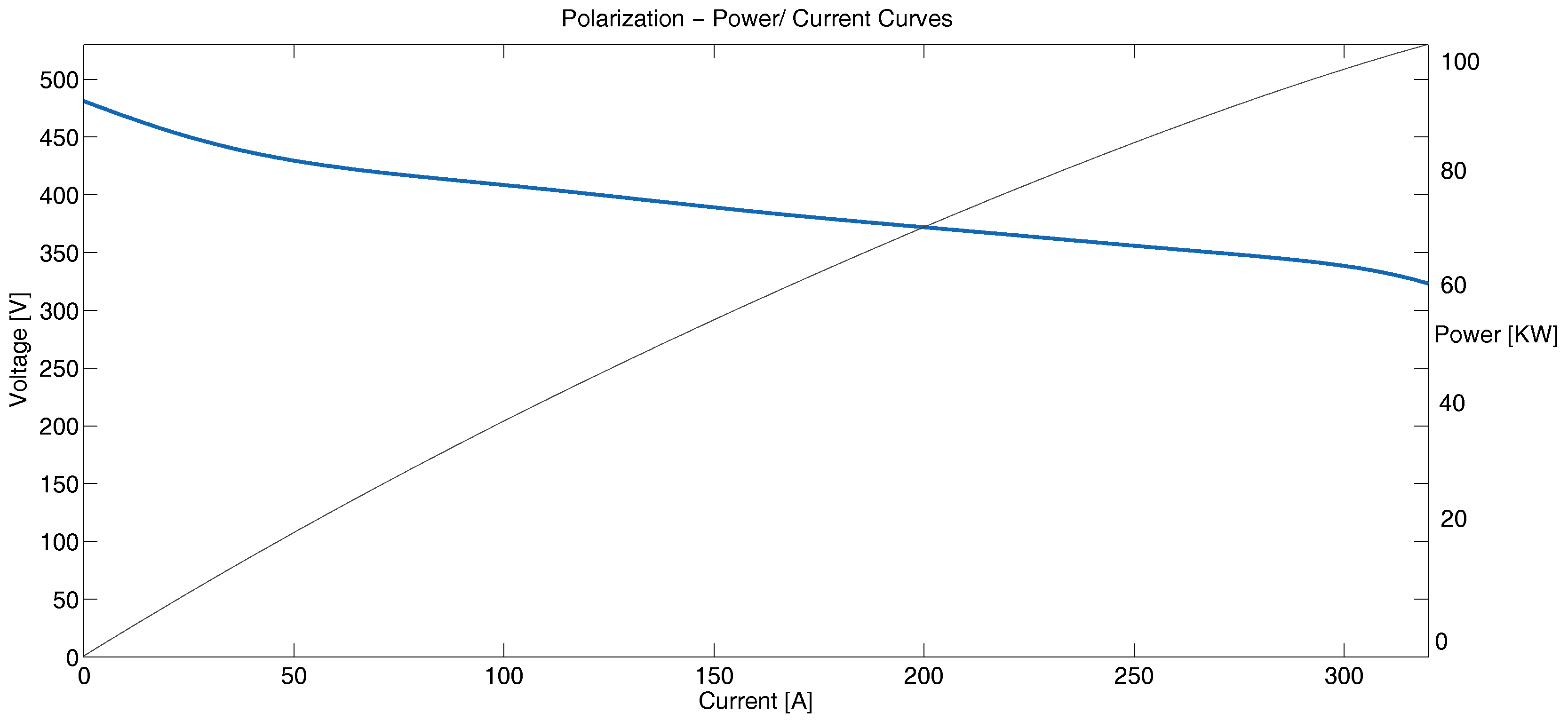
2.3. Fuel Cell Model

The PEMFC has two electrodes: The anode where the fuel is oxidized and the cathode where the oxidant is reduced [37]. The electrolyte simultaneously acts as an electrical insulator and a proton conductor. It also separates the cathode and anode reactions. Electrons go from the anode to the cathode through an external circuit generating electrical current, while protons do so through the electrolyte. In the cathode, electrons, protons, and oxidant are reduced, generating sub-products. Hydrogen is often used as an oxidizing agent and oxygen as reducing agent in this type of fuel cells.

The potential difference generated by a single unit or mono cell is less than one volt, so several mono-cells must be connected in series to obtain the appropriate voltage for the required application. However, although the fuel cell is the main part of a fuel cell system, the entire system typically involves the following subsystems:

• Supply of oxidant.
• Fuel supply.
• Heat management.
• Water management.
• Power conditioning, instrumentation, and controls.

The fuel and oxygen inlet lines to each cell are connected in parallel to achieve similar pressure in the anode and cathode. Impedance is a function of fuel pressure, membrane moisture, and catalyst status. To characterize the model to be used, we know that power is the product of current and potential. The power density is the product of the potential and current density, so it can be represented by:

$$p_{fc}=v_{fc}{i}_{fc}.$$

(11)

The power density is usually drawn with current density using the so-called polarization curves and indicate that there is a maximum power density that a fuel cell can reach. It is not always possible to operate the fuel cells at their maximum power levels. The polarization curve and power-current curve used in this work for the fuel cell are shown in Figure 2. In this work, we have taken the curve of the fuel cell for a BALLARD XD6 FCvelocity module fuel cell system, which is dimensionalized according to the maximum power of the driving profiles to be used, which are explained in the next section. Therefore, there is a maximum power that the cell can reach, because the efficiency of the fuel cell is directly proportional to the potential of the cell. Fuel cell efficiency is defined by:

$$n_{fc}=\frac{p_{fc}}{p_{H_2}}$$

(12)

where $p_{fc}$ is the electrical power produced and $p_{H_2}$ is the theoretical power associated with the hydrogen consumed, which is defined as

$$p_{H_2}=\frac{p_{fc}+p_{com}}{{\eta }_{therm}·{\eta }_{util}·{\eta }_{fci}}$$

(13)

where $p_{com}$ is the power that the compressor demands, ${\eta }_{therm}$ is thermodynamic efficiency (0.98 at 298 K), ${\eta }_{util}$ is the efficiency of cell use, defined as a relationship between the mass of fuel that reacted and the mass that entered in the fuel cell; and ${\eta }_{fci}$ is the efficiency of each cell, calculated as the relationship between the cell voltage $v_{fc}$, and the open-circuit voltage $E_{oc}$. This relationship can also be expressed as a function of cell voltage and current

$$n_{fc}=\frac{v}{1.482}\frac{i}{(i+i_{loss})}.$$

(14)

The losses of i, called $i_{loss}$ are usually small. Greater efficiency can be achieved with the same fuel cell, with significantly lower power density level. This means that for a required power, a fuel cell can be expanded (with a larger active area) and be more efficient [38].

An electric model characterizing the fuel cell can be obtained using voltage and current equations

$$u_{fc}=E_{oc}-u_{act}-u_{ohmic}$$

(15)

where $u_{fc}$ is the system voltage output, $u_{ohmic}$ is the voltage of ohmic losses, and $u_{act}$ is the activation voltage drop. $E_{oc}$, the open-circuit voltage, is defined by

$$E_{oc}=K_c[E_o+(T_{fc}-T_{ref})\frac{-{\alpha }_{Tref}}{zF}+{\displaystyle \frac{RT}{zF}}ln\left(P_{H_2}{P}_{O_2}^{1/2}\right)]$$

(16)

where ${\alpha }_{Tref}$ is a temperature constant, $E_o$ is the electromotive force under standard pressure conditions, $T_{ref}$ is the temperature of reference, $K_c$ is the rated voltage constant, $T_{fc}$ is the operating temperature, z is the electron transfer number, which can be obtained as shown in [39], $P_{H_2},P_{O_2}$ are the gas pressure, F is the Faraday constant and R is the gas constant. The activation drop, $u_{act}$, is given by:

$$u_{act}=\frac{1}{\tau s+1}N{A}_{nom}ln\left(\frac{i_{fc}}{i_o}\right)$$

(17)

where $\tau$ is the voltage time constant, and N is the number of cells. The ohmic voltage drop, $u_{ohmic}$ is expressed by:

$$u_{ohmic}=r_{internal}{i}_{fc}$$

(18)

where $i_{fc}$ is the cell output current and $r_{internal}$ is the inner resistance of fuel cell system. The parameters of the fuel cell stack are shown in

Table 4. HD 100 FCvelocity Ballard fuel cell parameters.

Parameter	Data
Maximum voltage	580 V
Maximum current	288 A
Number of cells	560
Operating temperature	330 ${}^{\circ }$K
Nominal air pressure	2.24 bar
Maximum power	100 kW
Mass	285 kg
Temperature of reference	298 ${}^{\circ }$K
Temperature constant	44.43
Cost	100 k€

. Finally, the hydrogen consumption is defined by:

$$m_{H_2}=\frac{N{M}_{H_2}i\lambda }{nF}$$

(19)

where $m_{H_2}$ is the mass of hydrogen consumed, $M_{H_2}$ is the molar mass of hydrogen, $\lambda$ is the ratio of excess hydrogen and n is the number of electrons acting on the reaction.

3. Driving Profiles

A driving cycle consists of a speed profile which defines the route that must follow the vehicle. Some types of vehicles track specific cycles, such as urban transport, which follow and predefined urban routes. Different driving cycles have been created that represent the driving conditions of vehicles with greater accuracy [40]. For example, the $ECE15$, which is the European cycle, whose main problem is the smooth accelerations; the USFTP 72 cycle, which represents the conditions of circulation in the Angeles; the USFTP 75, used for emissions certification in the USA.

However, in this paper we will present two specific driving cycles, the transport Driving Cycle in Buenos Aires (BADC), and the Manhattan Driving Cycle (Manhattan DC), because they are driving cycles designed for city buses, such as those indicated in Table 1, in which the driving conditions of these buses are considered. They have several stops and decelerations, which allows recovery of a significant amount of energy.

3.1. Buenos Aires City Driving Cycle

For the construction of the Buenos Aires Driving Cycle (BADC), 30 h of GPS data have been acquired, which are related to 51 bus trips covering a total of 313.6 km. The BADC was validated on a reference diesel bus widely used in Buenos Aires, and comparing the results obtained from fuel consumption to those reported by the bus line operator. The speed profile is shown in Figure 3, and its main characteristics are presented in

Table 5. BADC driving cycle parameters.

Parameter	Value
Total cycle time	1864 s
Average Speed	3.92 m/s
Maximum speed	15.6 m/s
Maximum acceleration	9.2155 × 10${}^{-5}$ m/s${}^2$
$e_v^{+}$	22,678.62 kJ
$e_v^{-}$	11,870.63 kJ

.

Using Equation (1), we can obtain the instantaneous power needed to follow this profile. The equation allows us to obtain the power values, $p_v^{+}$, which are the instantaneous values that need to be delivered to produce the movement. The sum of these power values, for the complete profile, becomes the energy needed to produce movement, $e_v^{+}$. We can also obtain the power values that we can recover by means of regenerative braking, $p_v^{-}$. Analogously, the total sum of these power values, for the complete profile, will be the energy recovered by braking $e_v^{-}$. In the same way, the equation allows us to obtain the maximum instantaneous power that must be contributed $p_{maxv}^{+}$, and the maximum instantaneous power that can be recovered from braking $p_{minv}^{-}$, which is useful for dimensionalizing the storage systems.

Using the ratio indicated in Equation (19), we can obtain the maximum amount of energy that can be recovered when there are no losses. For the BADC, this amount is 52.34%.

$$\%recovery=\frac{e_v^{-}}{e_v^{+}}.$$

(20)

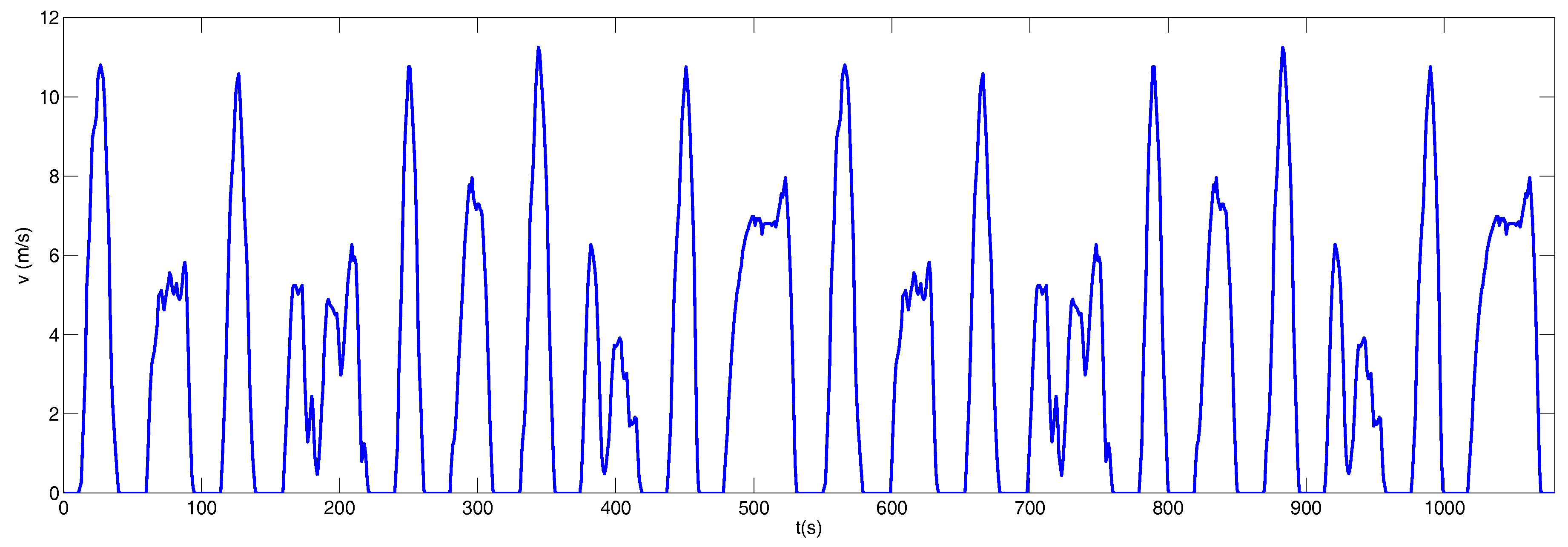
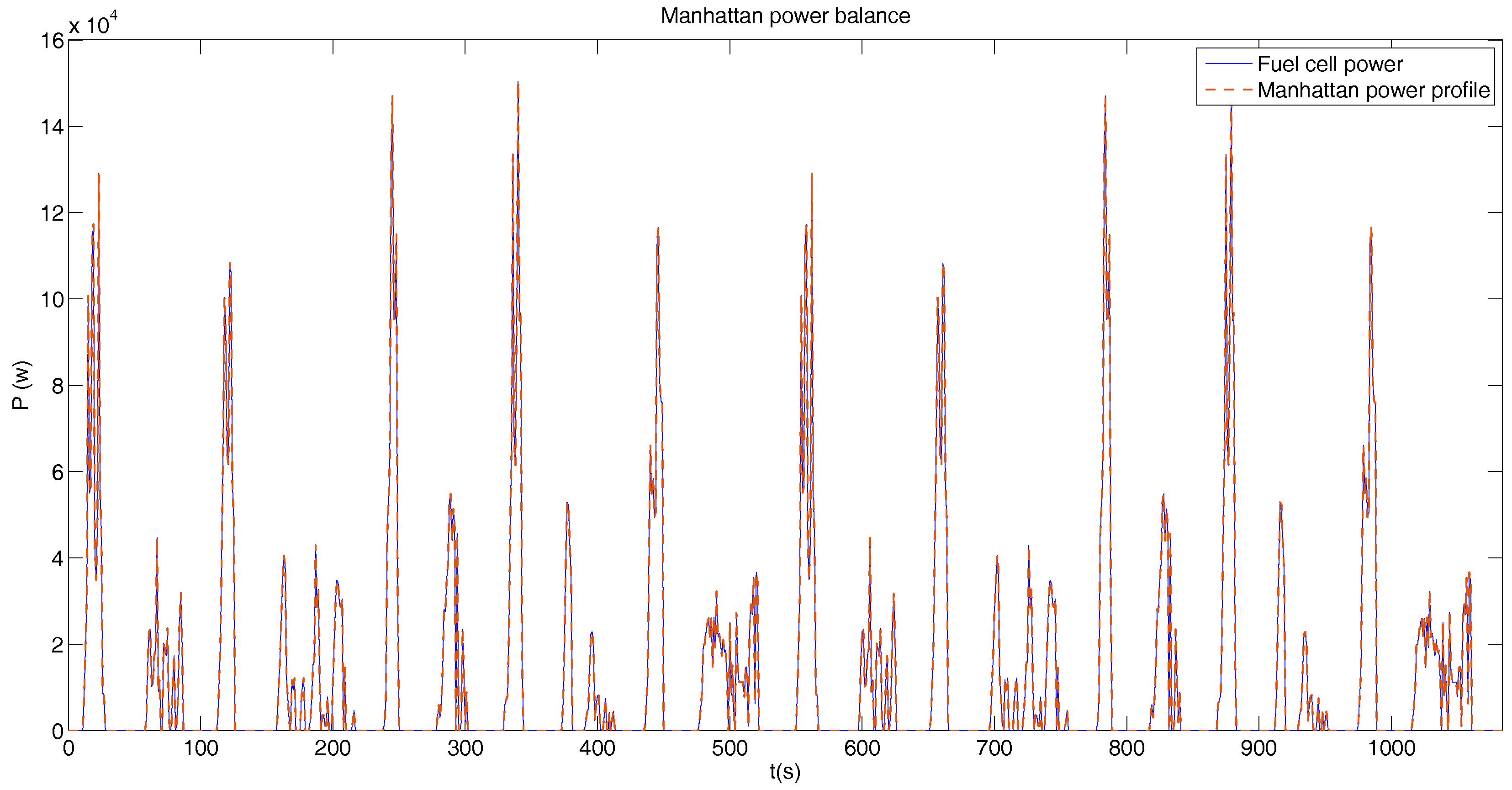
3.2. Manhattan Driving Cycle

This driving cycle used for bus testing in New York has a profile travel distance of 3.30 km, with a maximum acceleration of 2.04 ${\displaystyle \frac{m}{s^2}}$ and a driving time of 1089 s. Figure 4 shows the Manhattan profile velocity cycle.

Table 6. Manhattan Driving Cycle parameters.

Parameter	Value
Total cycle time	1089 s
Average Speed	3.033 m/s
Maximum speed	11.24 m/s
Maximum acceleration	2.044 m/${\mathrm{s}}^2$
$e_v^{+}$	13,747.04 kJ
$e_v^{-}$	8090.08 kJ

shows the most relevant parameters of the profile.

In the same way as for the BADC profile, and using ratio Equation (20), the maximum amount of energy that can be recovered from braking for this profile is 58.84%.

4. Dynamic Programming

Dynamic programming is a very powerful numerical tool for solving optimal control problems, as indicated in [41,42]. One of the advantages over other methods is that the solution of the optimal control can be found in the complete time horizon. However, in some cases the computational effort grows exponentially with the number of state variables and inputs of the dynamic system. When the problem includes state constraints, any control input trajectory is limited to keep the system operating in the space delimited by them.

The optimal problem for the energy management in vehicles is posed in a constant time interval, with fixed initial conditions and a speed profile known to priori. The proposed optimal control problem can be generically formulated considering the cost function

$$J=h_N\left(x\left(N\right)\right)+\sum _{k=0}^{N-1}{h}_k(x\left(k\right),u\left(k\right))$$

(21)

where the first term $h_N\left(x\left(N\right)\right)$, refers to the final cost. The second term $h_k(x\left(k\right),u\left(k\right))$, refers to the cost of reaching a proposed state $x\left(k\right)$, applying a control signal $u\left(k\right)$, in an instant k, considering that system dynamics is represented in discrete-time state space as

$$x(k+1)=f_k(x\left(k\right),u\left(k\right)).$$

(22)

Please note that second term of Equations (21) and (22) depend on k, therefore their value varies with each iteration.

In case of the vehicle energy system, the states, $x\left(k\right)$, are the battery SOC, the supercapacitor SOE, and the fuel cell energy $e_{fc}$, while $u\left(k\right)$ are the power of the elements $p_{sup}$, $p_{bat}$, $p_{fc}$, and $p_{break}$.

Then, the discrete-time model of the system is defined by

$$x_1(k+1)=SO{C}_{bat}\left(k\right)+{\displaystyle \frac{p_{bat}\left(k\right)}{e_{bat}}}$$

(23)

$$x_2(k+1)=So{E}_{sup}\left(k\right)+{\displaystyle \frac{p_{sup}\left(k\right)}{e_{sc}}}$$

(24)

$$x_3(k+1)=e_{fc}\left(k\right)+p_{fc}\left(k\right).$$

(25)

Excessive computational cost can be avoided by expressing the final system as follows. To make this reduction, the power ratio shown in Equation (2) is taken into account.

$$x_1(k+1)=SO{C}_{bat}\left(k\right)+{\displaystyle \frac{p_v\left(k\right)-p_{fc}\left(k\right)-p_{sup}\left(k\right)-p_{break}\left(k\right)}{e_{bat}}}.$$

(26)

$$x_2(k+1)=So{E}_{sup}\left(k\right)+{\displaystyle \frac{p_{sup}\left(k\right)}{e_{sc}}}.$$

(27)

Constraints will be imposed on the battery SOC and supercapacitor SOE, as state restrictions, as follows

$$0.4\le SO{C}_{bat}\left(k\right)\le 0.8$$

(28)

$$0\le So{E}_{sup}\left(k\right)\le 1$$

(29)

$$SO{C}_{bat,0}=SO{C}_{bat,N}$$

(30)

$$So{E}_{sup,0}=So{E}_{sup,N}$$

(31)

where $SO{C}_{bat,0}$, is the SOC of the battery at the initial instant and $SO{C}_{bat,N}$ is the SOC of the battery at the end of the driving cycle. In the same way $So{E}_{sup,0}$ is the SOE of supercapacitor at the initial instant and $So{E}_{sup,N}$ is the SOE of the supercapacitor at the end of the driving cycle.

The safety threshold [0.4, 0.8] applied to the battery SOC, which theoretically could vary in the ranges [0, 1] as the supercapacitor, is included to extend its useful life, avoiding deep discharges. Constraints on control signals, $u\left(k\right)$, are also included as follows

$$P_{lowerbat}\le P_{bat}\left(k\right)\le P_{maxbat}$$

(32)

$$P_{lowersup}\le P_{sup}\left(k\right)\le P_{maxsup}$$

(33)

$$P_{lowerfc}\le P_{fc}\left(k\right)\le P_{maxfc}.$$

(34)

The maximum and lower power and energy values will be taken from the tables indicated in the models of the elements.

4.1. Cost Function

When defining the particular expression of the cost function, Equation (21), for the energy management system, we will take into account the following considerations:

• The operational life of the elements.
• The amount of hydrogen consumed.

In the case of the operational life of elements, such as batteries, the parameters that are evaluated to characterize the main causes for degradation are: (a) temperature, (b) depth of discharge, and (c) rate of discharge [43,44,45,46,47,48,49]. Degradation can be avoided by limiting rapid power changes and preventing the instantaneous value from reaching the maximum value, which would result in deep discharges. In the case of the fuel cell, high current peaks and rapid variation in current should be avoided [38,50,51,52].

Finally, the cost function according to the control objectives is defined with the following terms.

• To preserve the operational life of the elements (state of health of the elements) abrupt variations

  (a)

  in the power delivered by the fuel cell $p_{fc}\left(k\right)-p_{fc}(k-1)$ and batteries $p_{bat}\left(k\right)-p_{bat}(k-1)$ and

  (b)

  in the SOC of the battery $SO{C}_{bat}\left(k\right)-SO{C}_{bat}(k-1)$,53], should be avoided [54].

• The amount of hydrogen consumed by the fuel cell, expressed as a function of the power delivered, $p_{fc}\left(k\right)$, which determines the economic cost should be minimized.

Thus, the cost function is finally defined as

$$\begin{array}{c}\hfill J=w_{u1}{[p_{bat}\left(k\right)-p_{bat}(k-1)]}^2+w_{u2}{[p_{fc}\left(k\right)-p_{fc}(k-1)]}^2+w_{SOH}{p}_{bat}{\left(k\right)}^2+\\ \hfill w_{soc}{[SO{C}_{bat}\left(k\right)-SO{C}_{bat}(k-1)]}^2+w_{\alpha }{p}_{fc}{\left(k\right)}^2\end{array}$$

(35)

where the weights $w_{\alpha }$, $w_{u1}$, $w_{u2}$, $w_{SOH}$, $w_{soc}$, have been determined based on of a sweep of these coefficients as explained in the following section.

4.1.1. Coefficient Sweep for BADC

Once the structure of the cost function was defined, we should proceed to make a sweeping of the weights to determine the Pareto front that allows choosing those that allow reduction of the power delivered by the fuel cell in order to reduce hydrogen consumption, as proposed in [55]. In addition, the one that allows a smoother variation of the SOC of the battery to preserve its useful life should be selected. To adjust the cost function coefficients based on sweeping of the weights, an initial sizing of the system is required to solve the control problem proposed in the previous section. This sizing is done with a storage element size shown in

Table 7. Initial sizing for the calculation of pareto coefficients.

Component	Mass	Power	Energy
Battery	8 kg	10.4 kW	368 Wh
Supercapacitor	12 kg	20.4 kW	27.6 Wh

. The reason for choosing this initial size of the storage system is that the literature recommends that the size of the storage system be about 30% of the size of the main source. The fuel cell used is the one detailed in Table 4.

It is considered that the sum of the weights $w_{\alpha }$, $w_{u1}$, $w_{u2}$, $w_{SOH}$, $w_{soc}$, will always satisfy

$$w_{\alpha }+w_{u1}+w_{u2}+w_{SOH}+w_{soc}=1$$

(36)

The coefficients $w_{u2}$ and $w_{\alpha }$, affect the behavior of the fuel cell and the $w_{u1}$, $w_{SOH}$, $w_{soc}$ coefficients affect the behavior of the battery. Then, it starts with a value of the coefficients $w_{u2}=0$ and $w_{\alpha }=0$, while the coefficients of the terms referring to the battery are maximum with a value of $w_{u1}=0.33$, $w_{SOH}=0.33$, and $w_{soc}=0.33$. In this first case, the condition of Equation (36) is fulfilled. In a second iteration, the coefficients related to the fuel cell take the values of $w_{u2}=0.05$ and $w_{\alpha }=0.05$, with an increase of 0.05 with respect to the first iteration. The coefficients related to the battery take the value of $w_{u1}=0.3$, $w_{SOH}=0.3$, and $w_{soc}=0.3$. All the coefficients related to the battery have the same value that is calculated by:

$$w_{u1}=w_{SOH}=w_{soc}={\displaystyle \frac{1}{3}}-{\displaystyle \frac{(w_{\alpha }+w_{u2})}{3}}$$

(37)

In this case, the second iteration also complies with Equation (35). In the last iteration with the increase of 0.05 to the fuel cell related coefficients in each new iteration, the coefficients have the values of $w_{u2}=0.4$, $w_{\alpha =0.4}$, $w_{u1}=0.067$, $w_{SOH}=0.067$, and $w_{soc}=0.067$. All combinations (iterations) of the coefficients can be seen in

Table 8. Variation in the weight of the cost function for BADC.

Weights					Energy
$w_{u2}$	$w_{u1}$	$w_{SOH}$	$w_{soc}$	$w_{\alpha }$	Battery (%)	Supercapacitor (%)	Fuel cell (%)
0	0.33	0.33	0.33	0	13.24	23.84	19.41
0.05	0.3	0.3	0.3	0.05	16.79	27.74	23.31
0.1	0.267	0.267	0.267	0.1	18.00	29.35	24.78
0.15	0.23	0.23	0.23	0.15	18.76	29.48	25.25
0.2	0.2	0.2	0.2	0.2	18.99	29.57	25.32
0.25	0.167	0.167	0.167	0.25	19.68	29.80	25.73
0.3	0.13	0.13	0.13	0.3	19.96	30.15	26.22
0.35	0.1	0.1	0.1	0.35	20.96	30.19	26.72
0.4	0.067	0.067	0.067	0.4	21.71	30.84	27.22

. For each of these combinations of coefficients, there is an amount of energy contributed by each element of the propulsion system. The power generated by the fuel cell, battery and supercapacitor must be equal to the power needed for motion fulfilling Equation (2). For a better understanding, the energy of each element will be expressed as a percentage. In the case of the battery and supercapacitor, this percentage will be the amount of energy they give to the system with respect to the maximum possible that they can recover in braking, calculated in Equation (20) for the BADC profile. As mentioned, the SOC and energy of these elements are equal at the beginning and at the end, being the energy recovered from the braking, equal to the energy delivered. In the case of the fuel cell, the percentage of energy saved by hybridization is shown compared to a pure fuel cell system without storage elements. These results, for each iteration of weights can also be observed in Table 8. In the last configuration of coefficients shown in Table 8, it is observed that there is the lowest fuel consumption with a fuel cell energy consumption reduction of 27.22%. In the same configuration, the power delivered by the battery is the highest in the table with 21.71%. Being one of the control objectives that the variation of the SOC is not abrupt, it is necessary to choose a configuration of weights in which the variation of the SOC is not the highest. For this reason, the configuration of coefficients chosen will be (a) $w_{\alpha }=0.3$, (b) $w_{u1}=0.13$, (c) $w_{u2}=0.3$, (d) $w_{SOH}=0.13$, (e) $w_{soc}=0.13$, where the power delivered by the battery is 19.96%, being the same lower than 21.71% which is the maximum value. In this configuration, the energy savings delivered by the fuel cell is 26.22%. As it can be seen, the fuel saving is still significant in this configuration, being only 1% less than the maximum saving case. This configuration of coefficients achieves a better balance of the proposed control objectives. Please note that the criterion for choosing the coefficients is based on the fact that the energy delivered by the battery is not the maximum and that the variation between the maximum consumption in the use of the fuel cell and the chosen value should be similar to 1%.

Figure 5 and Figure 6 illustrate the increase in fuel savings when the amount of power recovered by the storage elements increases for each combination of cost function coefficients. Figure 5 presents this relationship for the fuel cell and battery, while Figure 6 shows this relationship for the fuel cell and supercapacitors. Figure 5 shows in the lower left-hand corner, the case in which the coefficients take the values of $w_{\alpha }=0$, $w_{u1}=0.33$, $w_{u2}=0$, $w_{SOH}=0.33$, and $w_{soc}=0.33$. For this case, the energy reduction delivered by the fuel cell is 19.41%, while the energy recovered by the battery is 13.24% and for the supercapacitor is 23.84%. This is the case where the fuel cell delivers the most energy to the system. In the upper right corner, there is the case where the coefficients take a value of $w_{\alpha }=0.4$, $w_{u1}=0.067$, $w_{u2}=0.4$, $w_{SOH}=0.067$, and $w_{soc}=0.067$. For this case, the energy reduction delivered by the fuel cell is 27.22%, and the energy recovered by the battery is 21.71% and for the supercapacitor is 30.84%. This is the case where the fuel cell delivers the smallest amount of energy. The intermediate cases are taken from Table 8. In Figure 6, the same cases as for Figure 5 are shown, with the difference that the power delivered by the supercapacitor and not that of the battery is shown.

When the fuel cell delivers less energy to the movement, and the battery also delivers less energy (of the regenerative brake’s recovered power), due to the weights of the cost function, the supercapacitor delivers an increasing amount of energy when other sources are restricted. The indicated behavior between the supercapacitor and the fuel cell is shown in Figure 6.

4.1.2. Coefficient Sweep for Manhattan Driving Cycle

For the Manhattan Driving Cycle, the procedure is similar to BADC. The design of the propulsion system is the same as for the previous case. Once the cost function is known, we vary the weight tuning, to find the best combination between the use of its elements, focusing on hydrogen saving, and preserving the useful life of the elements.

The variation in the weights of the cost function is similar to that of the BADC profile, and a summary of the region of interest is shown in

Table 9. Variation in the weight of the cost function for Manhattan DC.

Weights					Energy
$w_{u2}$	$w_{u1}$	$w_{SOH}$	$w_{soc}$	$w_{\alpha }$	Battery (%)	Supercapacitor (%)	Fuel cell (%)
0	0.33	0.33	0.33	0	11.02	25.66	19.57
0.05	0.3	0.3	0.3	0.05	13.20	25.89	20.33
0.1	0.267	0.267	0.267	0.1	14.52	26.36	21.16
0.15	0.23	0.23	0.23	0.15	15.51	27.89	22.73
0.2	0.2	0.2	0.2	0.2	15.84	28.08	23.56
0.25	0.167	0.167	0.167	0.25	16.43	28.47	23.76
0.3	0.13	0.13	0.13	0.3	17.21	28.83	24.38
0.35	0.1	0.1	0.1	0.35	18.15	29.23	24.58
0.4	0.067	0.067	0.067	0.4	21.29	30.72	25.19

.

Figure 7 shows the behavior of the battery with respect to the fuel cell saving. In this profile, with the combination of coefficients $w_{\alpha }=0$, $w_{u1}=0.33$, $w_{u2}=0$, $w_{SOH}=0.33$, and $w_{soc}=0.33$, the energy delivered by the battery is 11.02%, the energy delivered by the supercapacitor is 25.66%, while the reduction in fuel cell use is 19.57%. This is the lower left-hand corner of Figure 7, which corresponds to the case where the fuel cell delivers the most energy to the movement. With the combination of coefficients $w_{\alpha }=0.4$, $w_{u1}=0.067$, $w_{u2}=0.4$, $w_{SOH}=0.067$, and $w_{soc}=0.067$, the energy delivered by the battery is 21.29%, the energy delivered by the supercapacitor is 30.72%, while the reduction in fuel cell use is 25.19%, which corresponds to the upper right-hand corner of Figure 7 and the case where the fuel cell delivers the least amount of energy to movement.

Figure 8 shows the behavior of the fuel cell saving and supercapacitors for the same cases in Figure 7, summarized in Table 9.

As for the BADC profile, with the latest configuration of coefficients from Table 9, the energy delivered by the battery is 21.19%, while the reduction in fuel cell usage is 25.19%. In this case, the fuel economy is maximum and the variation of the battery SOC is also highest. For this reason, to have a smaller variation in the SOC of the battery, we use the configuration of coefficients (a) $w_{\alpha }=0.2$, (b) $w_{u1}=0.2$, (c) $w_{u2}=0.2$, (d) $w_{SOH}=0.2$, (e) $W_{soc}=0.2$, where the energy delivered by the battery is 15.84% and the reduction in the use of the fuel cell is 23.56%. In this way, we have a smaller variation of the SOC, and the fuel saving is about 1% of the maximum possible.

5. Results

Considering BADC and Manhattan profiles as case studies, the power profile for each driving cycle will be simulated. The combination of power generated by the fuel cell, and the energy recovered by the ESS, should be sufficient to reach the power profile, derived from the velocity profile. Additionally, to the parameters shown in Table 2, Table 3 and Table 4, we will use for each profile the coefficients resulting from the sweeping of parameters of the cost function corresponding to each one. The control problem is the same as described in Section 4. When the mass of ESS is equal to zero, the power will be generated with the fuel cell only, and that will be a first case of analysis. In this first case, we must properly dimensionalize the fuel cell to reach the required velocity at all times. In a second case, we will use the ESS, as mentioned above. To properly dimensionalizing of the system, in Table 3 and Table 4, power and energy are expressed as a function of mass. Then, we will increase their mass to analyze the optimal configuration and price.

5.1. Fuel Cell Operation Only

For the proposed analysis, no batteries or supercapacitors is assumed. The fuel cell provides all the power needed to reach both profiles. The cost of power production for high volume cells is 1 €/W.

5.1.1. Buenos Aires Driving Cycle

For this profile, we will use a fuel cell system with a power of 200 kW, with a cost of 200 k€. In this case study, the fuel cell must be able to fulfill the highest power peaks. This is the reason for using a system of 200 kW of total power. Figure 9 shows the power profile derived from the BADC speed cycle and the power delivered by the fuel cell.

In red, we can see the power required to fulfill the speed profile. In blue, the instantaneous power delivered by the cell. The graphs in blue and red are the same, because they have the same power values at each instant. As it can be observed, with this fuel cell sizing, we can also fulfill the profile. Then, the total cost of the propulsion system to achieve the BADC profile with fuel cell operation will be 2000 k€.

5.1.2. Manhattan Driving Cycle

For this profile, we will use the same configuration of fuel cell than in BADC profile. The maximum power of the system will be 200 kW, whose cost is 200 k€. Figure 10 shows in red, the power derived from the Manhattan velocity profile, and in blue, the power delivered by the fuel cell system. The values of instantaneous power as for the previous case are the same, so the blue and red graphs are the same.

As in the previous case, with this dimensionalizing, we were able to reach the required speed. The cost of the propulsion system is 2000 k€.

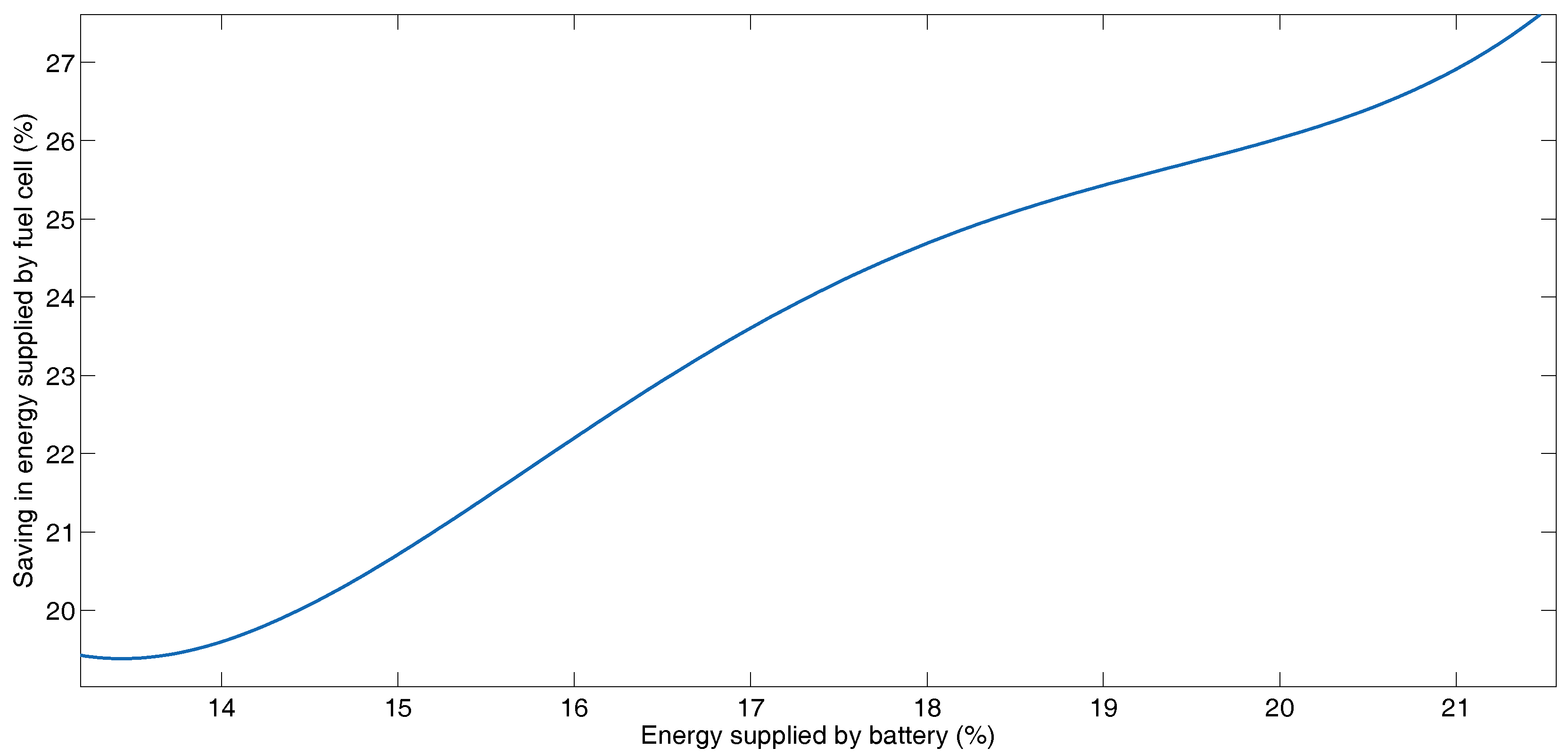
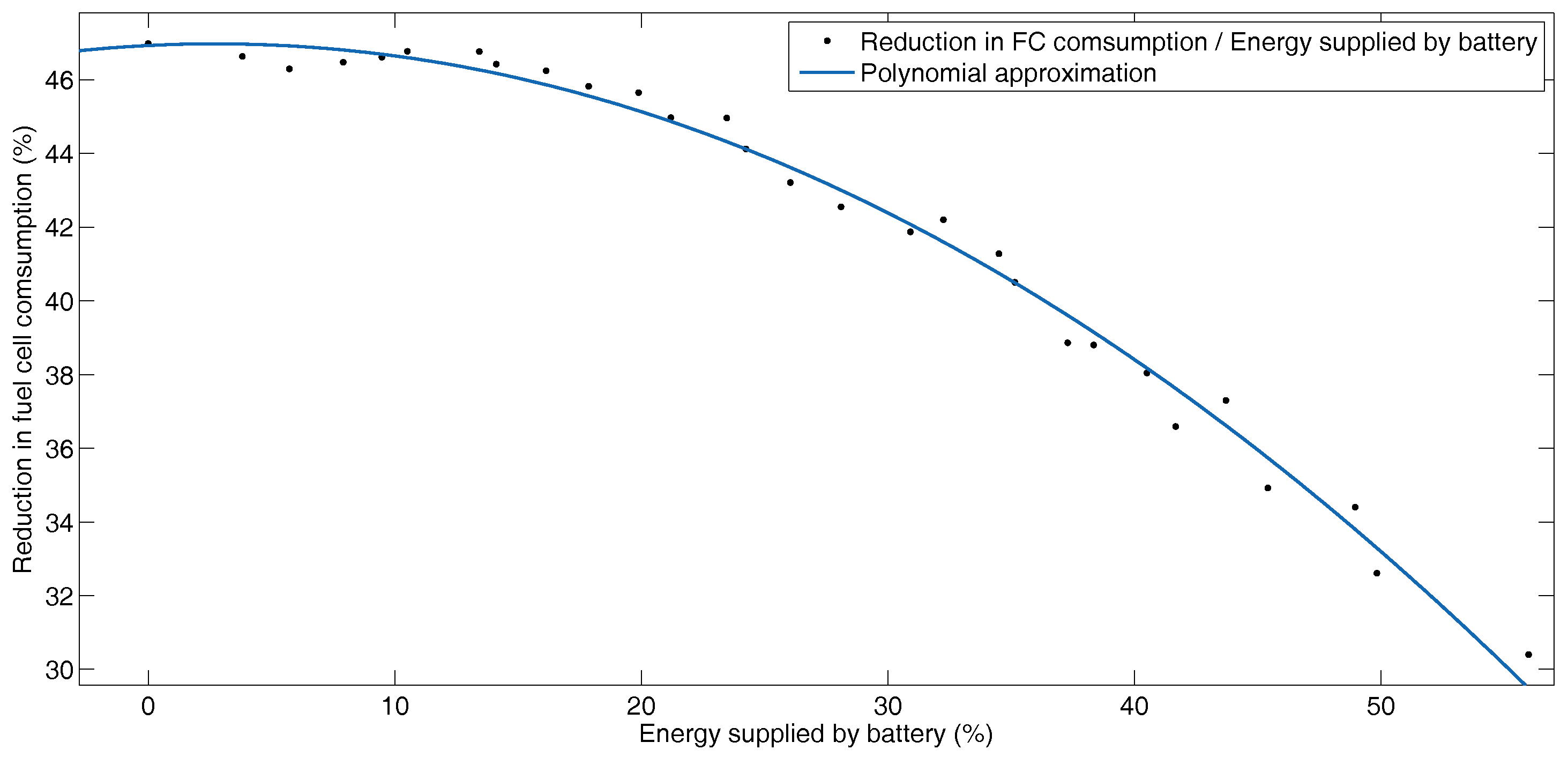
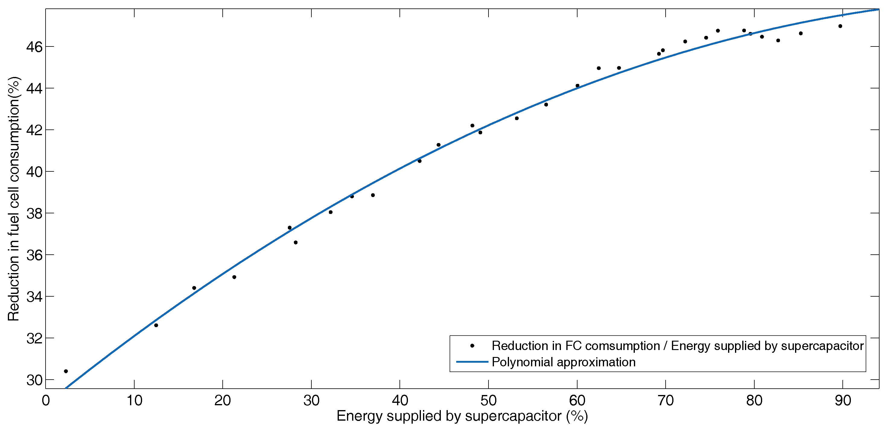
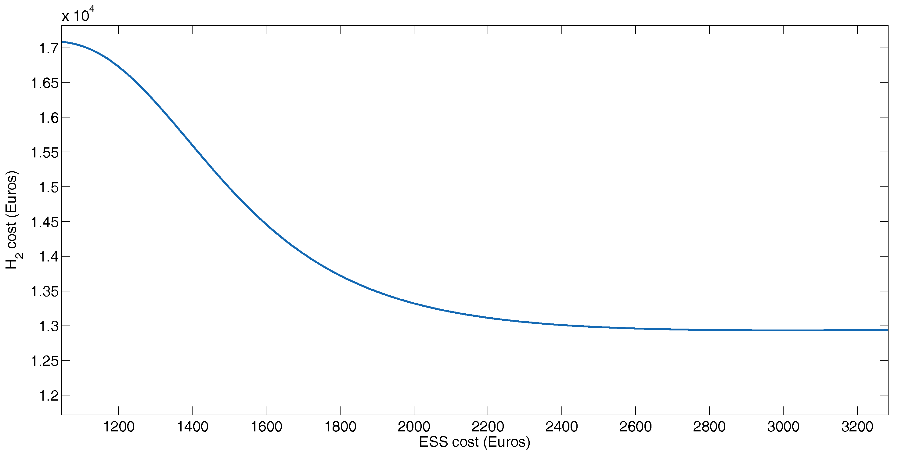
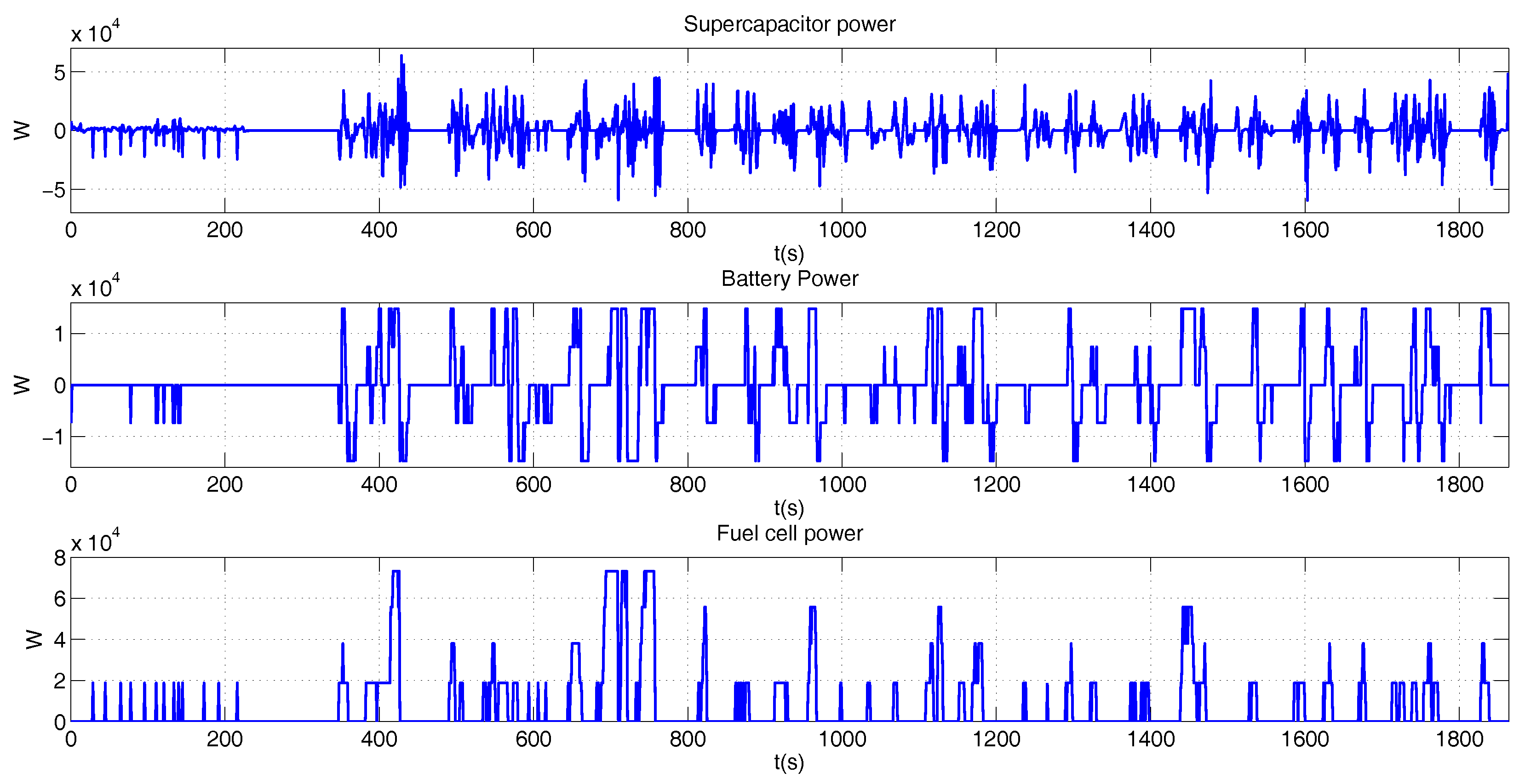
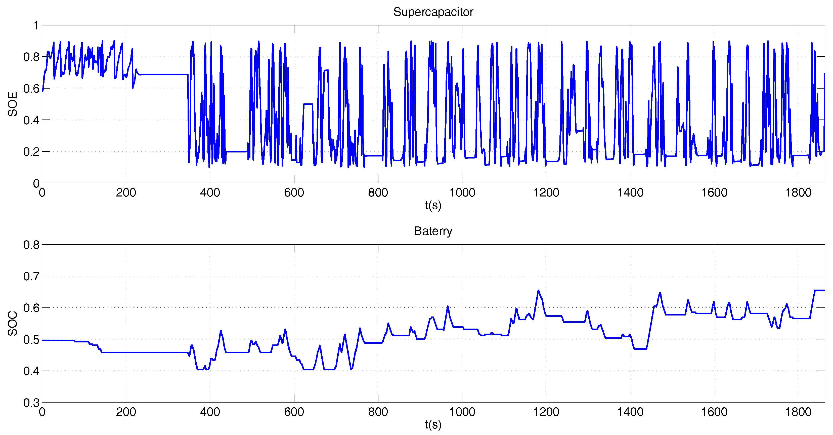
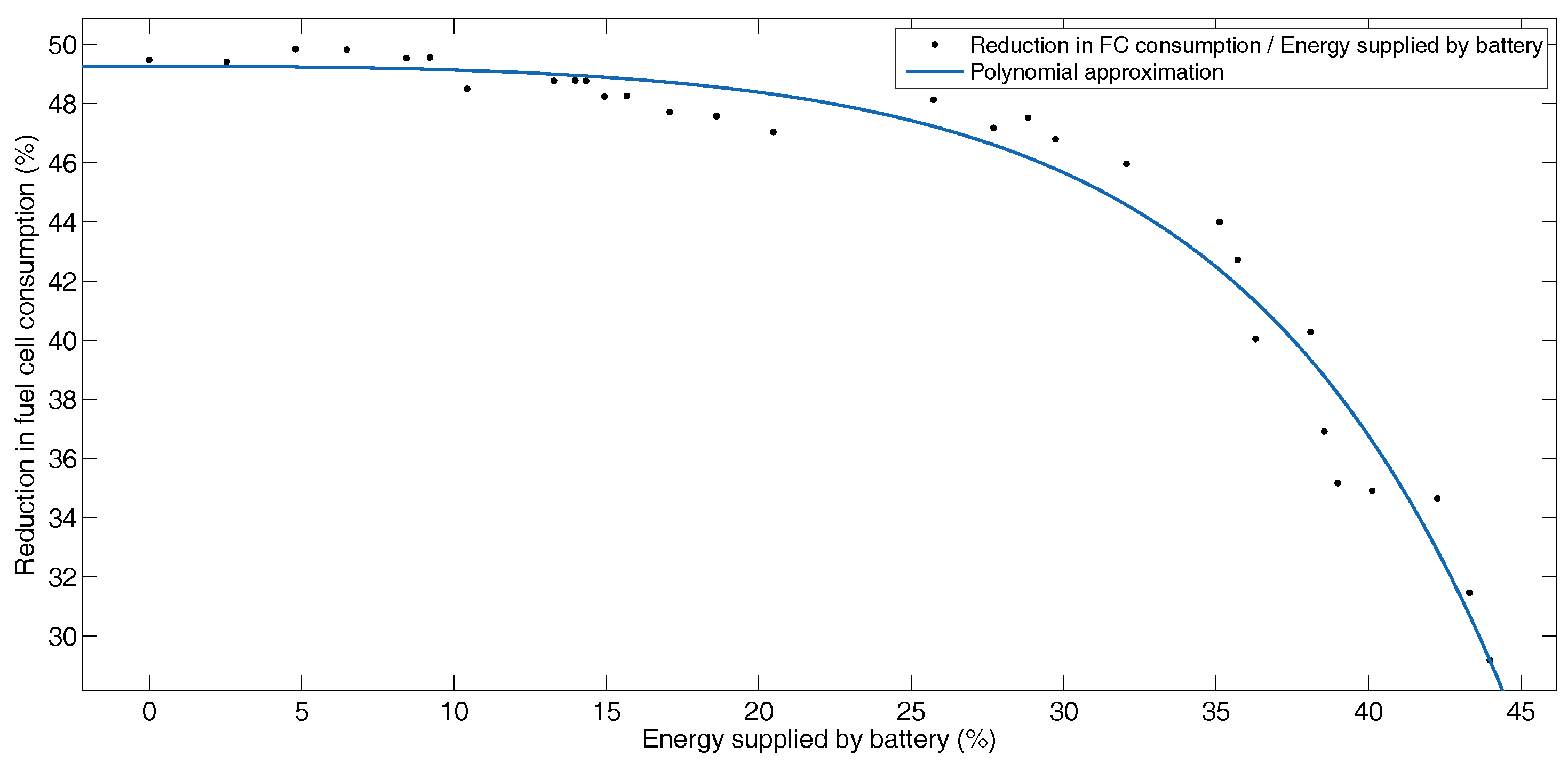
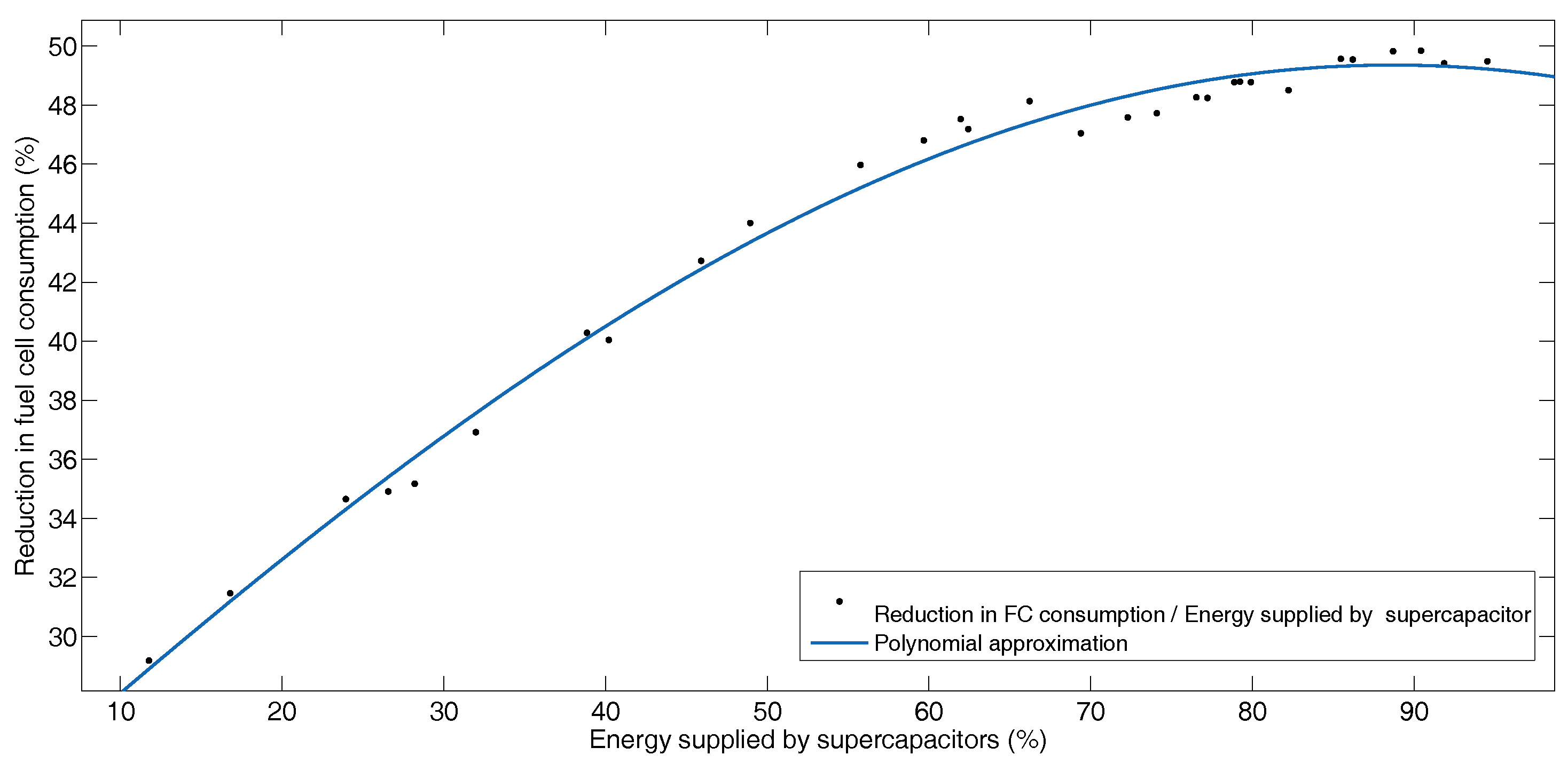
5.2. Hybrid Operation

When the mass of ESS increases, we can increase their capacity in power and energy and provide a significant reduction in fuel cell use. This will allow the fuel cell not to give the maximum power peaks of each profile, but to be able to give the average power of each one. The analysis of this variation, expressed in percentages of energy supplied by the storage elements and in the reduction of fuel cell use, will be presented below. Furthermore, the power profile of battery, supercapacitor, and fuel cell will also be plotted for a particular ESS mass value. Finally, in each profile, the monetary cost involved in increasing the power of the ESS will be reported in a graph.

BADC Driving Profile

During the sizing process, the total mass of the storage elements should be constant

$$m_{bat}+m_{sup}=m_{ess}$$

(38)

where $m_{ess}$ is the total mass and is constant and $m_{bat}$ and $m_{sup}$ are the ones that are going to vary. As indicated, supercapacitors allow recovery of a greater amount of power from braking, but they are more expensive than the battery. If the storage system is composed only of supercapacitors, the power of the fuel cell used in the system decreases, but the momentary cost of the storage system increases. Then, the objective is to find the mass of batteries and supercapacitors to reduce the cost of the storage system, but without forgetting the objectives of fuel economy control and SOC variation. For this reason, the case where the storage system has the lowest cost will not be optimal. This optimal case will depend on the compendium of the cost of the storage system and the other control objectives. A system with only supercapacitors ($m_{bat}=0$) is initially dimensionalized and mass is added to the batteries in each iteration. This is done to decrease the cost associated with the storage system in each iteration and to know how the fuel saving varies. Then, the initial configuration will be $m_{bat}=0$ and $m_{sup}=m_{ess}$. In order to fulfill with the power profile using the fuel cell described in Table 4, the minimum mass of supercapacitors should be 30 kg. Otherwise, if it is lower, the power profile is not fulfilled.

In the total mass, the mass of each element varies with respect to the other as follows. For example, in case 1: (a) When the mass of the supercapacitor is 30 kg, the battery mass should be 0 kg; (b) when the mass of the supercapacitor is 29 kg, the battery mass should be 1 kg. For each mass variation in batteries or supercapacitors, there is a new cost involved, and a new power and energy capacity. For example, for the same examples, in case 1, the cost of the battery is 0 €, while that of the supercapacitor is 2650 €. For case 2, the cost of the battery is 33.87 €, while the cost of the supercapacitor is 2561.67 €. As we can see, the total mass remains constant, but the economic value varies for each case. The final case will be when we have 28 kg of battery and 2 kg of supercapacitors, with a cost of 948.39 €, and 176.67 €, respectively. The configuration of 29 kg of batteries and 1 kg of supercapacitors is not considered, because with this configuration the power profile derived from the speed profile is not fulfilled. The weight, power and cost of the fuel cell remains constant for each configuration of batteries and supercapacitors in this scenario. The weight of the battery, supercapacitor and fuel cell, is added to the total mass for calculating the power profile, shown in Equation (1), to achieve a more realistic scenario. The cost of fuel cell FCveloCity-HD is 100 k€.

Contrarily to the case without hybridization, if the mass of the storage elements is different from 0, with a certain minimum value, we can reduce the size of the fuel cell. For the first case, where the mass of the supercapacitor is 30 kg ($m_{sup}=30$) and the mass of the battery is 0 kg ($m_{bat}=0$) the reduction in fuel cell usage is the highest with 46.98%. The cost of the storage system for this same case is also the highest with a value of 2650 €. For the last possible case, in which the mass of the supercapacitors is 2 kg ($m_{sup}=2$) and the mass of the battery is 28 kg ($m_{bat}=28$) the reduction in the consumption of the fuel cell is 30.4% and the storage system has the lowest cost, with 1125.05 €. Although 1125.05 €, is the cheapest cost of the storage system, the reduction in fuel cell usage is only 30.4%, while the battery delivers 55.98% of energy, being the same the highest of all configurations. This causes the variation of the SOC to be increased.

Figure 11 shows graphically the reduction in fuel cell consumption as a percentage of energy, compared to the percentage of energy recovered by the battery for each configuration. Even though the percentage of energy recovered by the battery increases, the reduction in fuel cell consumption decreases because the mass of the supercapacitors decreases. This shows that although the mass of the battery increases, the system does not absorb large peaks of power, so the fuel cell must provide more power. Figure 12 shows the same behavior of the fuel cell with the supercapacitor. Since supercapacitors have a high power density, they allow the system to recover the highest power peaks of the profile and the reduction in fuel cell consumption increases.

Figure 13 shows the variation of hydrogen consumption Equation (19) in relation to the cost of the storage system. The BADC profile has 1864 seconds of operation (31.06 min). A bus normally rolls 15 h per day. In one day, it would roll 29 times the profile, in one month it would roll 870 times and in a year 10.585 times.

In the Y axis of the Figure 13, the variation of the cost of hydrogen is indicated for a year of operation of the bus, and in the X axis the cost of the storage system is indicated. From the figure, it can be observed that with the lowest cost of the storage system (1125.05 €), a greater amount of hydrogen is consumed. This corresponds to the point of 28 kg of batteries and 2 kg of supercapacitors. Increasing the cost of the storage system reduces the consumption of hydrogen. In the maximum point the cost is 2650 € with 30 Kg of supercapacitors and 0 Kg of batteries.

However, it can be observed that from 2200 €, with the increase in the mass of the storage system, the decrease in hydrogen consumption is almost linear. This point corresponds to 9 Kg of batteries and 21 Kg of supercapacitors. According to this analysis, this will be the optimum point. In this configuration, the fuel cell consumption reduction is 45.82% (average reduction in fuel cell consumption for BADC mass variation), and 87.54% of the energy from the regenerative brake is recovered.

Therefore, for case 1 with a storage element cost of 2650 €, the energy delivered by the fuel cell is 53.02%. For the case 2 with a storage element cost of 2595.54 €, the energy delivered by the fuel cell is 53.37%. While for the last case, with a storage system cost of 1125.05 €, the fuel cell delivers 69.55% of energy to the movement. It can be observed how the fuel cell delivers a greater amount of energy, given the price decrease of the total storage system. In this sense, when we decrease the size of the supercapacitor system, the power can be recovered from regenerative braking decreases, and therefore, the fuel cell must provide more power to achieve the profile.

Figure 14 shows the supplied power by each element, while Figure 15, shows the battery SOC and supercapacitor SOE variation. The SOC has a slower variation than the SOE, due to the penalty of the cost function.

The sum of the battery, supercapacitor, and fuel cell powers in Figure 15 are equal to the power required to reach the BADC speed profile.

5.3. Manhattan Driving Profile

In the case of the Manhattan profile, the maximum power is higher than BADC. To satisfy Equation (38) and the initial condition of starting only with mass of supercapacitors ($m_{bat}=0$ and $m_{sup}=m_{ess}$), the minimum mass of supercapacitors must be 32 kg. With this initial mass, the control problem is feasible. In the first case must start with a mass of supercapacitors of 32 kg, and 0 kg of batteries, with a total cost of 2826.67 €. The fuel cell is the same as for the BADC profile, in cost and maximum power. The second case, to keep the total mass of 32 kg constant, we use 31 kg of supercapacitors and 1 kg of batteries, with a total cost of 2772.20 €, and so on in the other cases. The last case is with 29 kg of batteries and 3 kg of supercapacitors, with a cost of 1247.26 €. The configuration of 30 kg batteries and 2 kg supercapacitors is not possible, because the control problem is not feasible.

Figure 16 shows that the increase in the mass of the batteries and the decrease in the mass of the supercapacitors produces a decrease in the value of the reduction in the consumption of the fuel cell. Therefore, even though the energy recovered from battery for the braking increases, the fuel consumption increases.

Figure 17 shows the energy contributed to the movement by the supercapacitors and the reduction in fuel cell consumption. With a higher mass of supercapacitors, fuel consumption decreases, even if the battery mass is reduced.

Figure 18 shows in the X axis the cost of the storage system, while in the Y axis, the cost of the hydrogen consumption. In the same way as for the BADC, the duration of the Manhattan profile is 1089 s (18.15 min). In a year, a bus rolls 18,250 times the profile.

On the left side of the figure, can be observed that the cost of the storage system is lower, and hydrogen consumption is higher. The figure begins with a cost of 1247.26 € for the storage system and 18 K€ for hydrogen consumption. This is given with 29 Kg of batteries and 3 Kg of supercapacitors. Moving to the right of the figure, it is observed that as the cost of the storage system increases, the consumption of hydrogen decreases. With 32 kg of supercapacitors and 0 Kg of batteries, hydrogen consumption will be the lowest with almost 12.500 K€, while the cost of the storage system will be maximum with 2826.67 €. However, can be seen that from a value of 2200 €, the reduction in hydrogen consumption is almost linear. Then, the configuration of 12 Kg of batteries and 20 Kg of supercapacitors, is the optimal point of dimensionalizing. In this configuration, the fuel cell delivers 52.28% of the total energy of the movement.

In the optimal point, can be recovered 91.17% of the braking energy. The reduction of the fuel cell consumption is 47.72% (average reduction in fuel cell consumption for Manhattan Driving Cycle mass variation) and the cost is 2.173.12 €. As for the BADC, the case of the minimum cost was not taken into account as the optimal case because the energy delivered by the battery is the maximum and increases the variation of the SOC.

Figure 19 shows the power of each propulsion system element for the desired configuration, in addition Figure 20 presents the SOC and SOE variation.

In the same way, as for the previous case, the SOC variation is softer than SOE, due to the penalization conditions imposed on the cost function for the battery. Also, the sum of the three instantaneous powers reach the power required for the Manhattan speed profile.

6. Conclusions

In the considered HEV, the propulsion system without the use of energy storage elements requires a fuel cell system capable of generating all the power required for the BADC profile and Manhattan in each case. This means that the cost is high, as it is 200 k€, in each case (only fuel cell system). The inclusion of energy storage elements such as batteries and supercapacitors allows us to reduce fuel cell usage and reduce fuel cell size. For both profiles, the fuel cell can be dimensionalized with 100 kW of power instead of 200 kW, with a cost of 100 k€. Then, the increase in mass on ESS allows reduction of the consumption of hydrogen from the fuel cell. With higher mass of supercapacitors, greater savings in fuel consumption and reduction in power generated by the fuel cell are achieved. In the same way, the cost of the storage system is higher. For this reason, it is concluded that for both profiles the pure use of supercapacitors allows greater savings of hydrogen, but makes the storage system more expensive. The inclusion of batteries allows this cost to be reduced, but at the same time increases the use of the fuel cell.

A larger battery size allows the SOC to vary less abruptly, which helps to improve the operational life of the batteries. Several mass configurations of the storage elements were simulated to find the best cost of the storage system compared with a maximum quantity (supercapacitor system only), and at the same time, reduce the hydrogen consumption. In this way, we can take advantage of the battery’s energy density and supercapacitor power density characteristics. For the BADC speed profile, the optimal configuration was 9 Kg of batteries, and 21 Kg of supercapacitors. In this case, the energy recovered by the ESS is 87.54%, while the energy delivered by the fuel cell is 54.18%. The reduction of the cost, with the configuration (most expensive case), where only supercapacitors are presented as an ESS system, is 18.52%. For the Manhattan speed profile, the optimal configuration was 12 Kg of batteries, and 20 Kg of supercapacitors. In this case, the energy recovered by the ESS is 91.17 %, while the energy delivered by the fuel cell is 52.28%. The reduction of the cost, with the configuration (most expensive case), where only supercapacitors are presented as an ESS system, is 23.12%.

The behavior of the system with increasing mass of the storage elements is similar in both profiles. Its inclusion can be considered a significant contribution to hydrogen savings, and improves fuel cell efficiency.

As future work, additional objectives will be considered as the battery and fuel life degradation following the ideas proposed in [56] as well as the effect of the uncertainty to include robustness in the sizing.

References

1. Jia, S.; Peng, H.; Liu, S.; Zhang, X. Review of Transportation and Energy Consumption Related Research. J. Transp. Syst. Eng. Inf. Technol. 2009, 9, 6–16. [Google Scholar] [CrossRef]
2. Mahlia, T.; Saidur, R.; Memon, L.; Zulkifli, N.; Masjuki, H. A review on fuel economy standard for motor vehicles with the implementation possibilities in Malaysia. Renew. Sustain. Energy Rev. 2010, 14, 3092–3099. [Google Scholar] [CrossRef]
3. Sciarretta, A.; Guzzella, L. Control of hybrid electric vehicles. IEEE Control Syst. 2007, 27, 60–70. [Google Scholar] [CrossRef]
4. Mesbahi, T.; Khenfri, F.; Rizoug, N.; Chaaban, K.; Bartholomeüs, P.; Moigne, P.L. Dynamical modeling of Li-ion batteries for electric vehicle applications based on hybrid Particle Swarm–Nelder–Mead (PSO–NM) optimization algorithm. Electr. Power Syst. Res. 2016, 131, 195–204. [Google Scholar] [CrossRef]
5. Hu, X.; Moura, S.J.; Murgovski, N.; Egardt, B.; Cao, D. Integrated Optimization of Battery Sizing, Charging, and Power Management in Plug-In Hybrid Electric Vehicles. IEEE Trans. Control Syst. Technol. 2016, 24, 1036–1043. [Google Scholar] [CrossRef] [Green Version]
6. Hoke, A.; Brissette, A.; Smith, K.; Pratt, A.; Maksimovic, D. Accounting for Lithium-Ion Battery Degradation in Electric Vehicle Charging Optimization. IEEE J. Emerg. Sel. Top. Power Electron. 2014, 2, 691–700. [Google Scholar] [CrossRef]
7. Redelbach, M.; Özdemir, E.D.; Friedrich, H.E. Optimizing battery sizes of plug-in hybrid and extended range electric vehicles for different user types. Energy Policy 2014, 73, 158–168. [Google Scholar] [CrossRef] [Green Version]
8. Sakti, A.; Michalek, J.J.; Fuchs, E.R.; Whitacre, J.F. A techno-economic analysis and optimization of Li-ion batteries for light-duty passenger vehicle electrification. J. Power Sources 2015, 273, 966–980. [Google Scholar] [CrossRef]
9. Hemi, H.; Ghouili, J.; Cheriti, A. Combination of Markov chain and optimal control solved by Pontryagin’s Minimum Principle for a fuel cell/supercapacitor vehicle. Energy Convers. Manag. 2015, 91, 387–393. [Google Scholar] [CrossRef]
10. Zou, Z.; Cao, J.; Cao, B.; Chen, W. Evaluation strategy of regenerative braking energy for supercapacitor vehicle. ISA Trans. 2015, 55, 234–240. [Google Scholar] [CrossRef] [PubMed]
11. Rodatz, P.; Paganelli, G.; Sciarretta, A.; Guzzella, L. Optimal power management of an experimental fuel cell/supercapacitor-powered hybrid vehicle. Control Eng. Pract. 2005, 13, 41–53. [Google Scholar] [CrossRef]
12. Ayad, M.; Becherif, M.; Henni, A. Vehicle hybridization with fuel cell, supercapacitors and batteries by sliding mode control. Renew. Energy 2011, 36, 2627–2634. [Google Scholar] [CrossRef]
13. Shen, J.; Dusmez, S.; Khaligh, A. Optimization of Sizing and Battery Cycle Life in Battery/Ultracapacitor Hybrid Energy Storage Systems for Electric Vehicle Applications. IEEE Trans. Ind. Inform. 2014, 10, 2112–2121. [Google Scholar] [CrossRef]
14. Choi, M.E.; Lee, J.S.; Seo, S.W. Real-Time Optimization for Power Management Systems of a Battery/Supercapacitor Hybrid Energy Storage System in Electric Vehicles. IEEE Trans. Veh. Technol. 2014, 63, 3600–3611. [Google Scholar] [CrossRef]
15. Thounthong, P.; Chunkag, V.; Sethakul, P.; Davat, B.; Hinaje, M. Comparative Study of Fuel-Cell Vehicle Hybridization with Battery or Supercapacitor Storage Device. IEEE Trans. Veh. Technol. 2009, 58, 3892–3904. [Google Scholar] [CrossRef]
16. Hannan, M.; Azidin, F.; Mohamed, A. Hybrid electric vehicles and their challenges: A review. Renew. Sustain. Energy Rev. 2014, 29, 135–150. [Google Scholar] [CrossRef]
17. Hemi, H.; Ghouili, J.; Cheriti, A. A real time fuzzy logic power management strategy for a fuel cell vehicle. Energy Convers. Manag. 2014, 80, 63–70. [Google Scholar] [CrossRef]
18. Fotouhi, A.; Yusof, R.; Rahmani, R.; Mekhilef, S.; Shateri, N. A review on the applications of driving data and traffic information for vehicles energy conservation. Renew. Sustain. Energy Rev. 2014, 37, 822–833. [Google Scholar] [CrossRef]
19. Hu, X.; Murgovski, N.; Johannesson, L.M.; Egardt, B. Optimal Dimensioning and Power Management of a Fuel Cell; Battery Hybrid Bus via Convex Programming. IEEE/ASME Trans. Mechatron. 2015, 20, 457–468. [Google Scholar] [CrossRef]
20. Sharaf, O.Z.; Orhan, M.F. An overview of fuel cell technology: Fundamentals and applications. Renew. Sustain. Energy Rev. 2014, 32, 810–853. [Google Scholar] [CrossRef]
21. Fatás, E.; Pérez-Flores, J.C.; Ocón, P. Pilas de combustible: una alternativa limpia de producción de energía. Revista Española de Física 2013, 27, 26–34. [Google Scholar]
22. Tie, S.F.; Tan, C.W. A review of energy sources and energy management system in electric vehicles. Renew. Sustain. Energy Rev. 2013, 20, 82–102. [Google Scholar] [CrossRef]
23. Ren, G.; Ma, G.; Cong, N. Review of electrical energy storage system for vehicular applications. Renew. Sustain. Energy Rev. 2015, 41, 225–236. [Google Scholar] [CrossRef]
24. Gao, L.; Dougal, R.A.; Liu, S. Power enhancement of an actively controlled battery/ultracapacitor hybrid. IEEE Trans. Power Electron. 2005, 20, 236–243. [Google Scholar] [CrossRef]
25. Schupbach, R.M.; Balda, J.C.; Zolot, M.; Kramer, B. Design methodology of a combined battery-ultracapacitor energy storage unit for vehicle power management. In Proceedings of the 34th Annual Power Electronics Specialist Conference, Acapulco, Mexico, 15–19 June 2003; Volume 1, pp. 88–93. [Google Scholar] [CrossRef]
26. Nielson, G.; Emadi, A. Hybrid energy storage systems for high-performance hybrid electric vehicles. In Proceedings of the 2011 IEEE Vehicle Power and Propulsion Conference, Chicago, IL, USA, 6–9 September 2011; pp. 1–6. [Google Scholar] [CrossRef]
27. Qu, X.; Wang, Q.; Yu, Y. Power Demand Analysis and Performance Estimation for Active-Combination Energy Storage System Used in Hybrid Electric Vehicles. IEEE Trans. Veh. Technol. 2014, 63, 3128–3136. [Google Scholar] [CrossRef]
28. Chen, Z.; Mi, C.C.; Xu, J.; Gong, X.; You, C. Energy Management for a Power-Split Plug-in Hybrid Electric Vehicle Based on Dynamic Programming and Neural Networks. IEEE Trans. Veh. Technol. 2014, 63, 1567–1580. [Google Scholar] [CrossRef]
29. Jeong, J.; Kim, N.; Lim, W.; Park, Y.I.; Cha, S.W.; Jang, M.E. Optimization of power management among an engine, battery and ultra-capacitor for a series HEV: A dynamic programming application. Int. J. Automot. Technol. 2017, 18, 891–900. [Google Scholar] [CrossRef]
30. Sabri, M.M.; Danapalasingam, K.; Rahmat, M. A review on hybrid electric vehicles architecture and energy management strategies. Renew. Sustain. Energy Rev. 2016, 53, 1433–1442. [Google Scholar] [CrossRef]
31. Wu, G.; Zhang, X.; Dong, Z. Powertrain architectures of electrified vehicles: Review, classification and comparison. J. Frankl. Inst. 2015, 352, 425–448. [Google Scholar] [CrossRef]
32. Feroldi, D.; Serra, M.; Riera, J. Energy management strategies based on efficiency map for fuel cell hybrid vehicles. J. Power Sources 2009, 190, 387–401. [Google Scholar] [CrossRef]
33. Carignano, M.G.; Adorno, R.; van Dijk, N.; Nieberding, N.; Nigro, N.; Orbaiz, P. Assessment of Energy Management Strategies for a Hybrid Electric Bus. In Proceedings of the 5th International Conference on Engineering Optimization, Iguassu Falls, Brazil, 19–23 June 2016. [Google Scholar]
34. Feroldi, D.; Carignano, M. Sizing for fuel cell/supercapacitor hybrid vehicles based on stochastic driving cycles. Appl. Energy 2016, 183, 645–658. [Google Scholar] [CrossRef]
35. Aditya, J.P.; Ferdowsi, M. Comparison of NiMH and Li-ion batteries in automotive applications. In Proceedings of the Vehicle Power and Propulsion Conference, Harbin, China, 3–5 September 2008; pp. 1–6. [Google Scholar]
36. Parvini, Y.; Siegel, J.B.; Stefanopoulou, A.G.; Vahidi, A. Supercapacitor electrical and thermal modeling, identification, and validation for a wide range of temperature and power applications. IEEE Trans. Ind. Electron. 2016, 63, 1574–1585. [Google Scholar] [CrossRef]
37. Hoogers, G. Fuel Cell Technology Handbook; CRC Press: Boca Raton, FL, USA, 2002. [Google Scholar]
38. Barbir, F. PEM Fuel Cells: Theory and Practice; Academic Press: Cambridge, MA, USA, 2013. [Google Scholar]
39. Zhou, R.; Zheng, Y.; Jaroniec, M.; Qiao, S.Z. Determination of the electron transfer number for the oxygen reduction reaction: from theory to experiment. ACS Catal. 2016, 6, 4720–4728. [Google Scholar] [CrossRef]
40. Tzirakis, E.; Pitsas, K.; Zannikos, F.; Stournas, S. Vehicle emissions and driving cycles: comparison of the Athens driving cycle (ADC) with ECE-15 and European driving cycle (EDC). Glob. NEST J. 2006, 8, 282–290. [Google Scholar]
41. Bellman, R. Dynamic programming; Dover Publications: Mineola, NY, USA, 2003. [Google Scholar]
42. Bertsekas, D.P.; Bertsekas, D.P.; Bertsekas, D.P.; Bertsekas, D.P. Dynamic Programming and Optimal Control; Athena Scientific: Belmont, MA, USA, 1995; Volume 1. [Google Scholar]
43. Haifeng, D.; Xuezhe, W.; Zechang, S. A new SOH prediction concept for the power lithium-ion battery used on HEVs. In Proceedings of the Vehicle Power and Propulsion Conference, Dearborn, MI, USA, 7–11 September 2009; pp. 1649–1653. [Google Scholar]
44. Zou, C.; Manzie, C.; Nešić, D.; Kallapur, A.G. Multi-time-scale observer design for state-of-charge and state-of-health of a lithium-ion battery. J. Power Sources 2016, 335, 121–130. [Google Scholar] [CrossRef]
45. Ouyang, M.; Feng, X.; Han, X.; Lu, L.; Li, Z.; He, X. A dynamic capacity degradation model and its applications considering varying load for a large format Li-ion battery. Appl. Energy 2016, 165, 48–59. [Google Scholar] [CrossRef] [Green Version]
46. Wang, J.; Liu, P.; Hicks-Garner, J.; Sherman, E.; Soukiazian, S.; Verbrugge, M.; Tataria, H.; Musser, J.; Finamore, P. Cycle-life model for graphite-LiFePO4 cells. J. Power Sources 2011, 196, 3942–3948. [Google Scholar] [CrossRef]
47. Hu, X.; Johannesson, L.; Murgovski, N.; Egardt, B. Longevity-conscious dimensioning and power management of the hybrid energy storage system in a fuel cell hybrid electric bus. Appl. Energy 2015, 137, 913–924. [Google Scholar] [CrossRef]
48. Johannesson, L.; Murgovski, N.; Ebbesen, S.; Egardt, B.; Gelso, E.; Hellgren, J. Including a battery state of health model in the HEV component sizing and optimal control problem. IFAC Proc. Vol. 2013, 46, 398–403. [Google Scholar] [CrossRef]
49. Ebbesen, S.; Elbert, P.; Guzzella, L. Battery State-of-Health Perceptive Energy Management for Hybrid Electric Vehicles. IEEE Trans. Veh. Technol. 2012, 61, 2893–2900. [Google Scholar] [CrossRef]
50. Das, V.; Padmanaban, S.; Venkitusamy, K.; Selvamuthukumaran, R.; Blaabjerg, F.; Siano, P. Recent advances and challenges of fuel cell based power system architectures and control—A review. Renew. Sustain. Energy Rev. 2017, 73, 10–18. [Google Scholar] [CrossRef]
51. Dicks, A.; Rand, D.A.J. Fuel Cell Systems Explained; Wiley Online Library: Hoboken, NJ, USA, 2018. [Google Scholar]
52. Kongkanand, A.; Mathias, M.F. The priority and challenge of high-power performance of low-platinum proton-exchange membrane fuel cells. J. Phys. Chem. Lett. 2016, 7, 1127–1137. [Google Scholar] [CrossRef] [PubMed]
53. Li, L.; You, S.; Yang, C.; Yan, B.; Song, J.; Chen, Z. Driving-behavior-aware stochastic model predictive control for plug-in hybrid electric buses. Appl. Energy 2016, 162, 868–879. [Google Scholar] [CrossRef]
54. Song, Z.; Hofmann, H.; Li, J.; Hou, J.; Han, X.; Ouyang, M. Energy management strategies comparison for electric vehicles with hybrid energy storage system. Appl. Energy 2014, 134, 321–331. [Google Scholar] [CrossRef]
55. Sockeel, N.; Shi, J.; Shahverdi, M.; Mazzola, M. Pareto Front Analysis of the Objective Function in Model Predictive Control Based Power Management System of a Plug-in Hybrid Electric Vehicle. In Proceedings of the 2018 IEEE Transportation Electrification Conference and Expo (ITEC), Long Beach, CA, USA, 13–15 June 2018; pp. 1–6. [Google Scholar]
56. Sockeel, N.; Shi, J.; Shahverdi, M.; Mazzola, M. Sensitivity Analysis of the Battery Model for Model Predictive Control: Implementable to a Plug-In Hybrid Electric Vehicle. World Electr. Veh. J. 2018, 9, 45. [Google Scholar] [CrossRef]
Figure 1. Vehicle architecture.
Energies 12 00925 g001
Figure 2. Polarization and power-current curve of fuel cell.
Energies 12 00925 g002
Figure 3. BADC driving cycle.
Energies 12 00925 g003
Figure 4. Manhattan Driving Cycle.
Energies 12 00925 g004
Figure 5. Saving in energy supplied by fuel cell and energy supplied by batteries for the different combination of coefficients of the cost function for BADC.
Energies 12 00925 g005
Figure 6. Saving in energy supplied by fuel cell and energy supplied by supercapacitor for the different combination of coefficients of the cost function for BADC.
Energies 12 00925 g006
Figure 7. Saving in energy supplied by fuel cell and energy supplied batteries for the different combination of coefficients of the cost function for Manhattan Driving Cycle.
Energies 12 00925 g007
Figure 8. Saving in energy supplied by fuel cell and energy supplied batteries for the different combination of coefficients of the cost function for Manhattan Driving Cycle.
Energies 12 00925 g008
Figure 9. Power profile BADC with only fuel cell operation.
Energies 12 00925 g009
Figure 10. Power profile Manhattan with only fuel cell operation.
Energies 12 00925 g010
Figure 11. Reduction in fuel cell consumption versus energy supplied by battery for BADC profile.
Energies 12 00925 g011
Figure 12. Reduction in fuel cell consumption versus energy supplied by supercapacitor for BADC profile.
Energies 12 00925 g012
Figure 13. Cost of the storage and power delivered by fuel cell system in BADC profile.
Energies 12 00925 g013
Figure 14. Power of the propulsion system for the BADC profile.
Energies 12 00925 g014
Figure 15. SOC and SOE for the BADC profile.
Energies 12 00925 g015
Figure 16. Reduction in fuel cell consumption versus energy supplied by battery for Manhattan profile.
Energies 12 00925 g016
Figure 17. Reduction in fuel cell consumption versus energy supplied by supercapacitor for Manhattan profile.
Energies 12 00925 g017
Figure 18. Cost of the storage system in Manhattan profile.
Energies 12 00925 g018
Figure 19. Power of the propulsion system for the Manhattan profile.
Energies 12 00925 g019
Figure 20. SOC and SOE for the Manhattan profile.
Energies 12 00925 g020