Intelligent Control of Wind-Assisted PHEVs Smart Charging Station

 , , ,
, , ,  , ,
, ,
Abstract
:1. Introduction
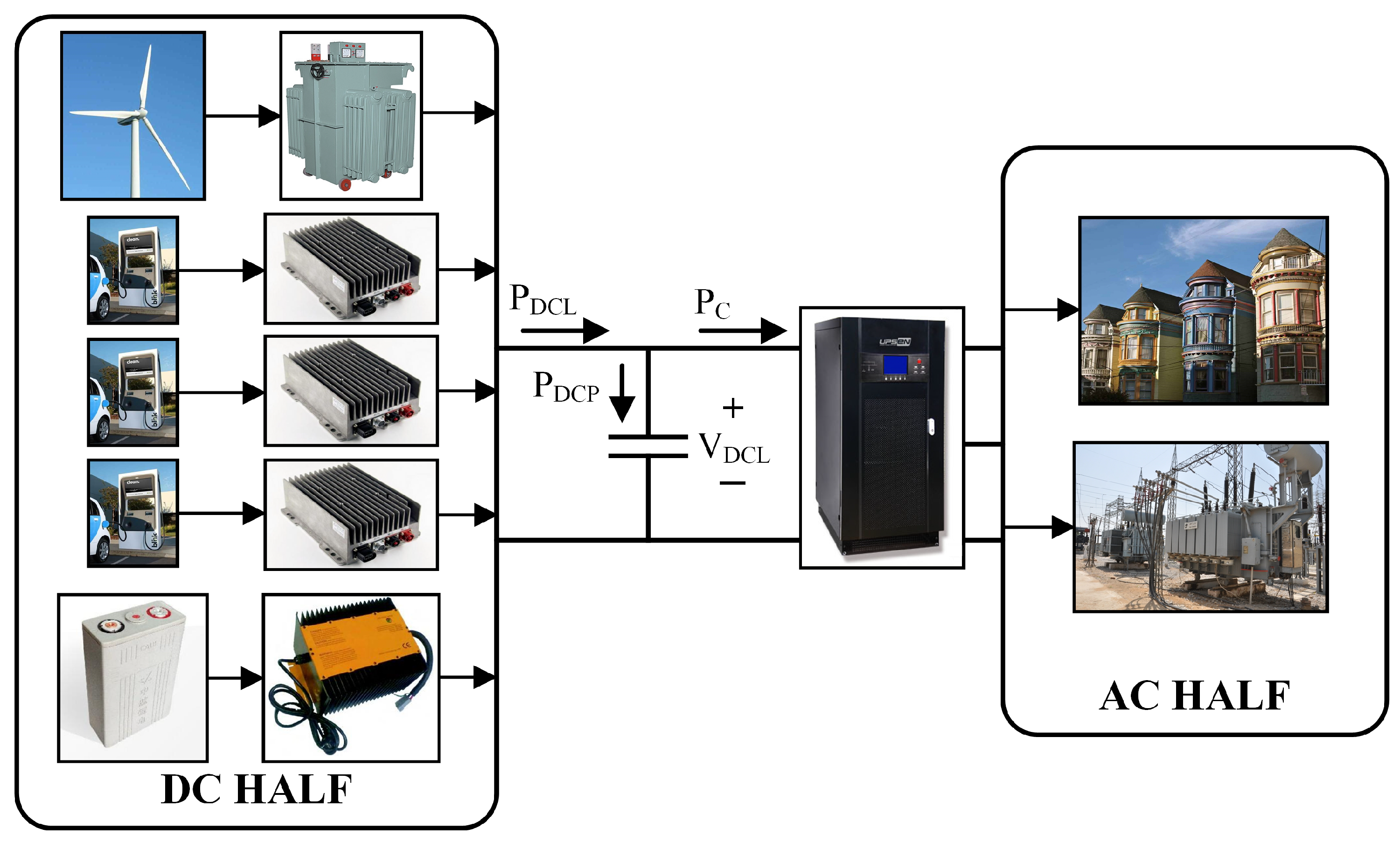
2. Proposed Charging Station Description
DC-Link Voltage Sensing
3. Control of System Components
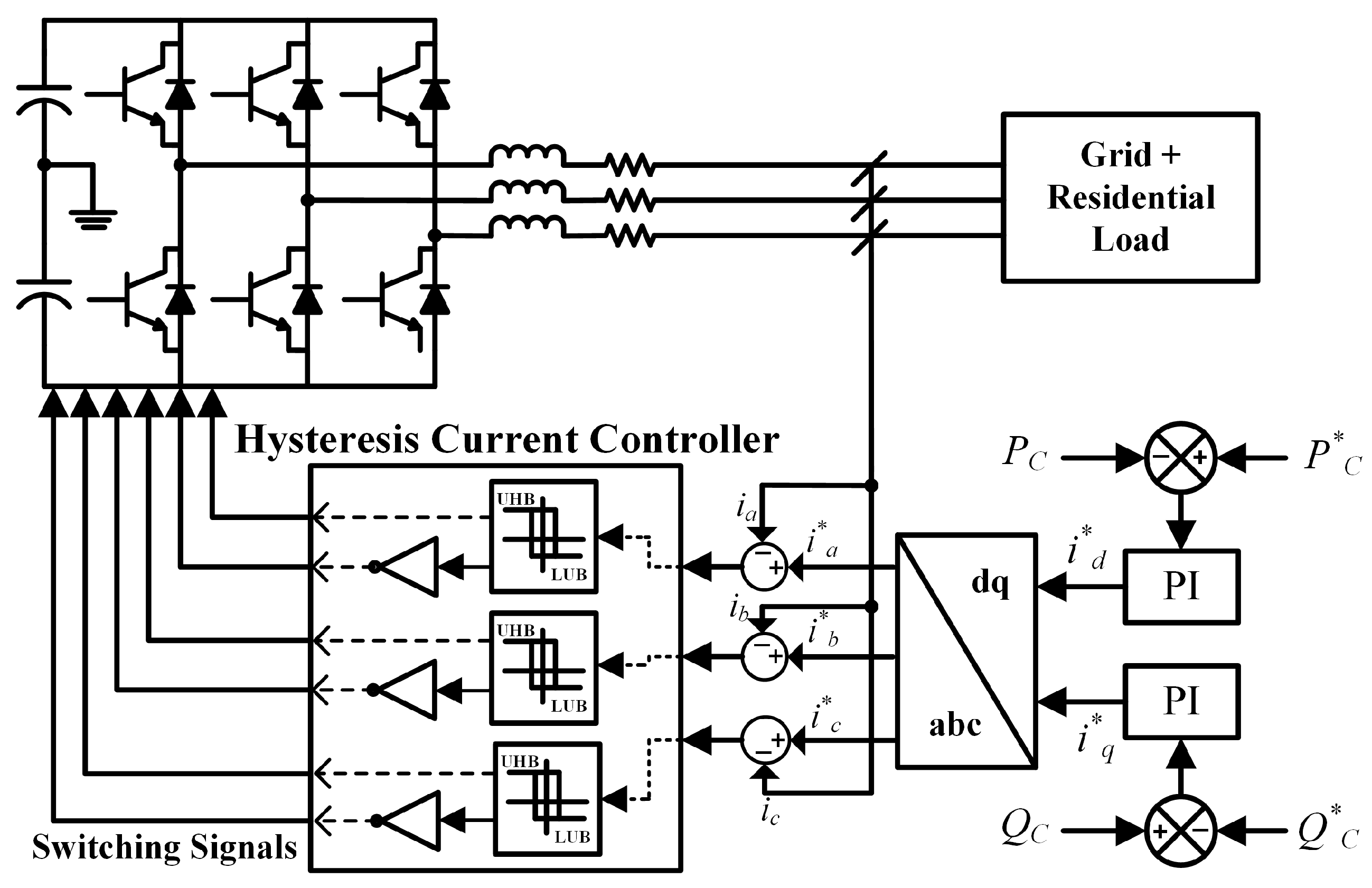
3.1. DC/AC Bi-Directional Converter
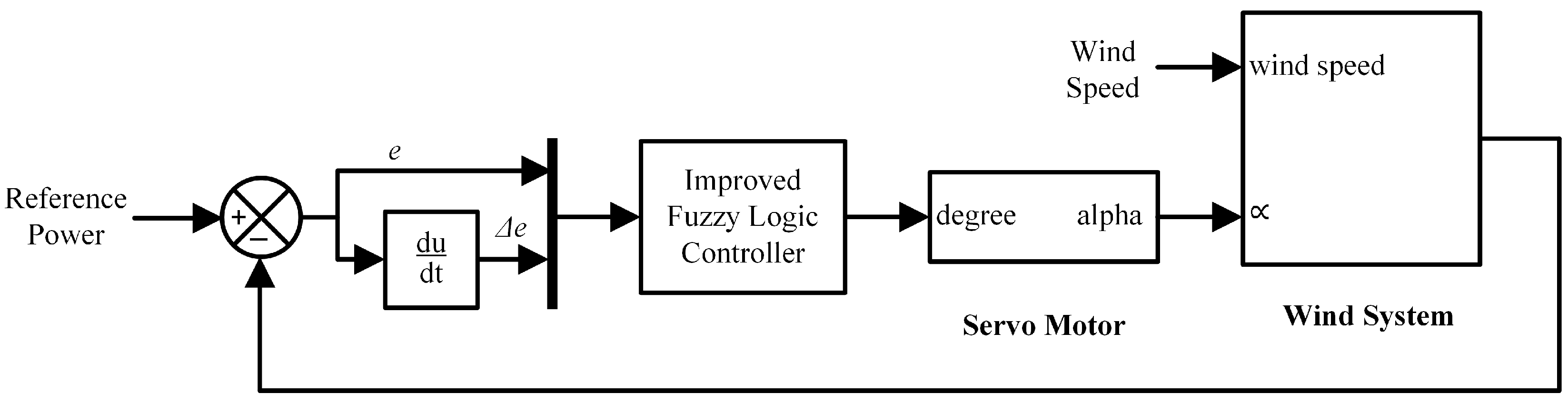
3.2. PMSG and MSWT (MPPT) Boost Converter Control
4. Energy Management System (EMS)
4.1. Operations of EMS
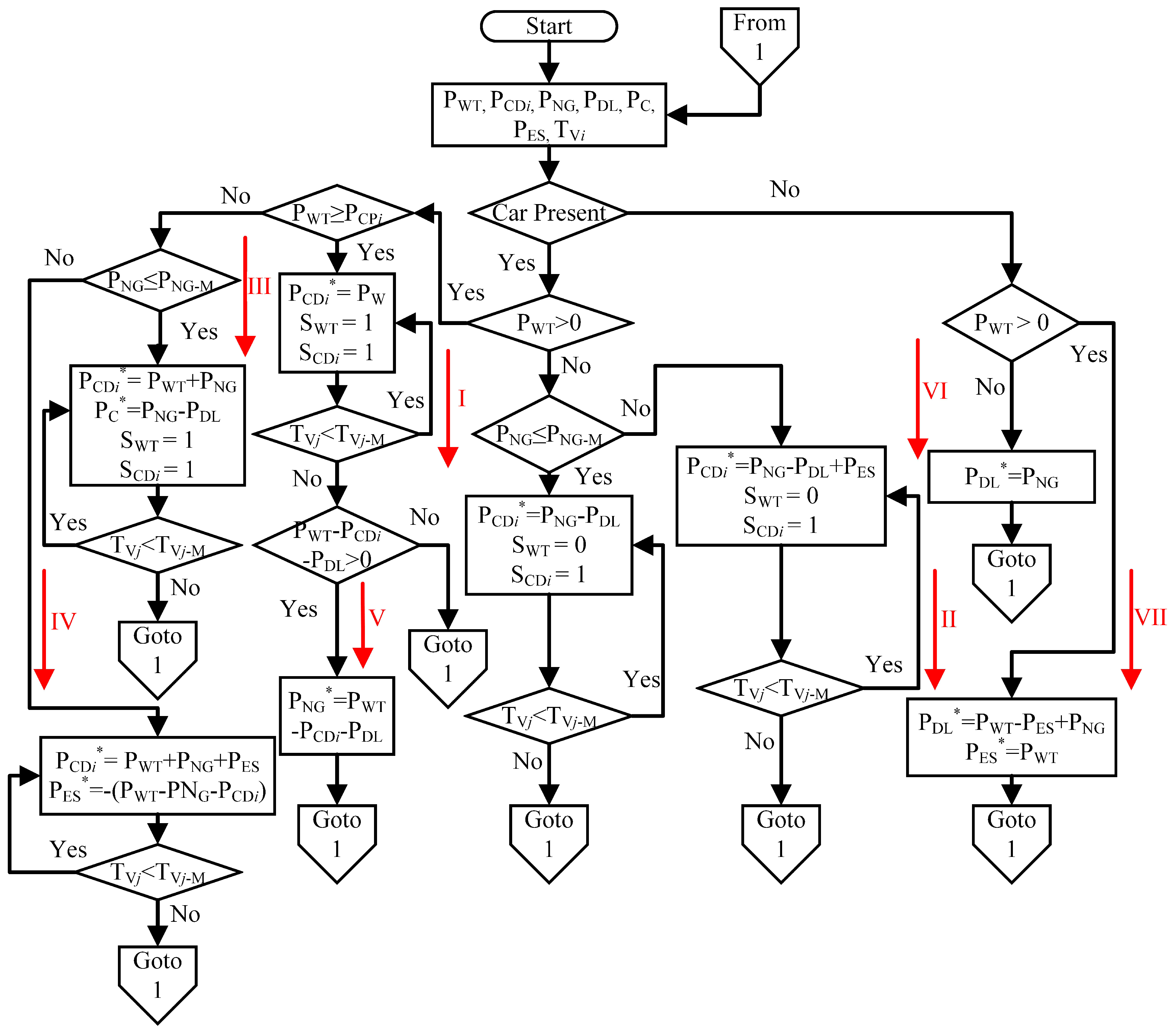
4.1.1. Generalized Algorithm
- Read the target values of , and .
- Check whether the car is present, or, if not present, then go to the next step, otherwise move to step number 13.
- Once it has been confirmed that the car is present, then get the status of the WT output power. If power is available from the WT system, then it moves to the next step; otherwise go to step 10.
- Check the power of the WT output. If it is greater than the charging point demanded (i.e., ), then go to the next step, otherwise go to step 7.
- All the WT generated power is being supplied to the corresponding charging point. Here, it will be tested if either the battery is fully charged or not (i.e., ). If, yes, then moveto the next step, otherwise keep this condition ‘on’ until the battery has been fully charged.
- Once the battery has been fully charged, then pay attention to the power balance equation and check any excess power in the system. If the condition is true, then the excess power will be delivered to NG, else go to step 1.
- Now, check the status of NG power; if it is less than the maximum power rating of NG, then move to the next step, otherwise go to step 9.
- Deliver the required power to the CD. The CD demand is shared between the WT and NG. Check whether the battery is fully charged or not. If, yes, then go to step 1, otherwise follow the target mechanism until the battery has been fully charged. Then go to step 1.
- As CP demand is not satisfied by the WT and NG, so, the remaining power is fulfilled by the ESS. It will charge the battery until it has been fully charged.
- As WT power is not available, here, the status of power demand left for NG will determine whether it is greater than its highest rating of power or not. If yes, then move to next step, else go to step 12.
- The acquired power for CDs is delivered under the sharing of NG and WT. So, charge the battery until its maximum SOC, then move to 1.
- The required power of CDs has been fulfilled by the contribution of NG, WT and ESS. So, charge the battery until its SOC reaches its maximum value, then go to step 1.
- As PHEV is not present, the WT output power will be checked. If PWT is greater than zero, it means that all the WT power is being delivered to DL and ESS charging. Go to step 1, else go to the next step.
- The DL demand is satisfied by the contribution of NG and ESS without incorporating WT. Go to step 1.
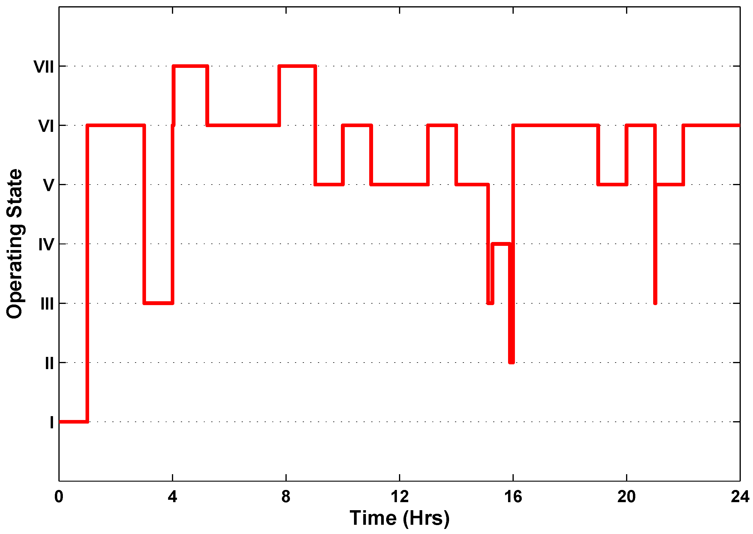
4.1.2. Operating States
5. Results and Discussion
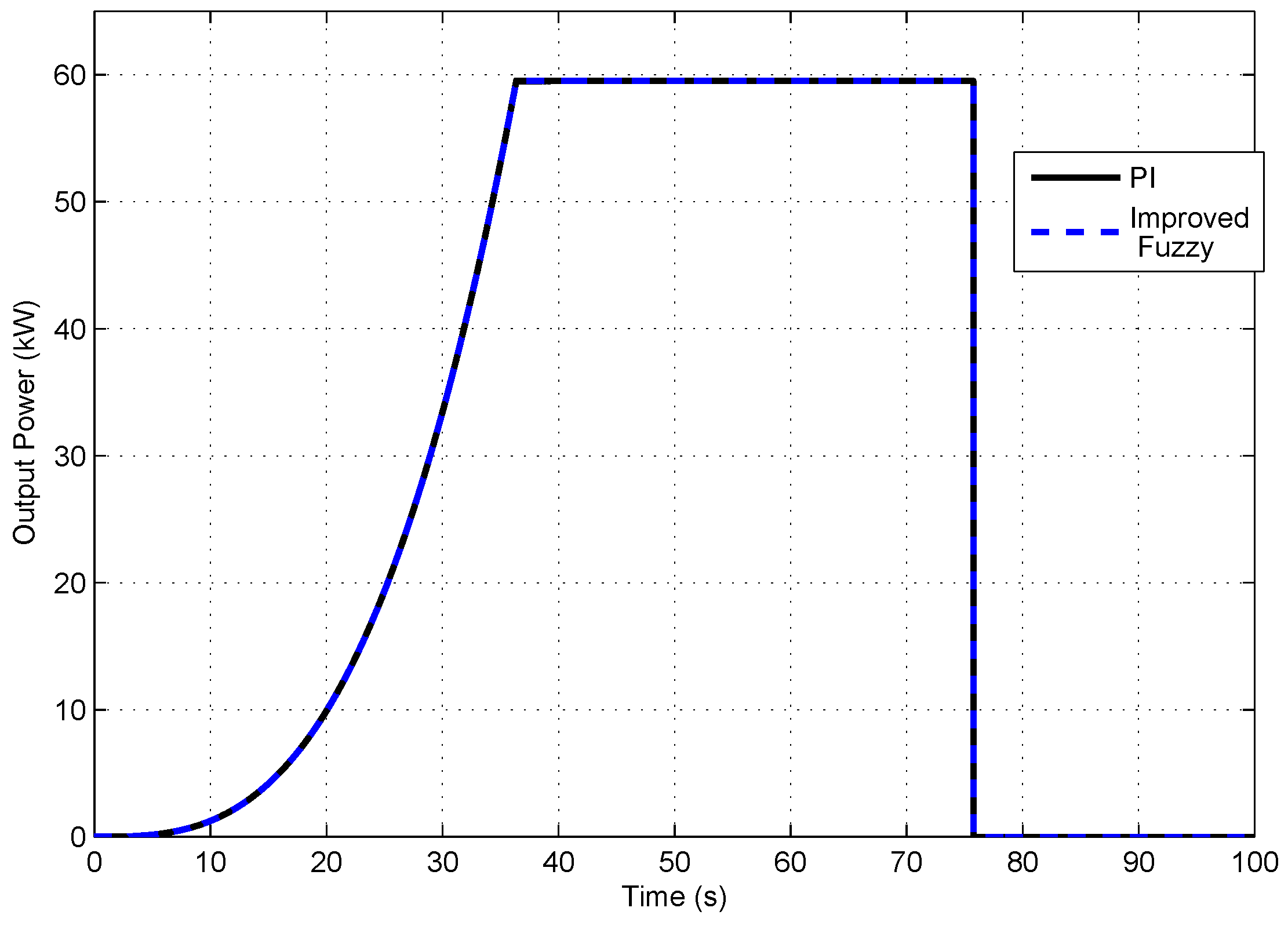
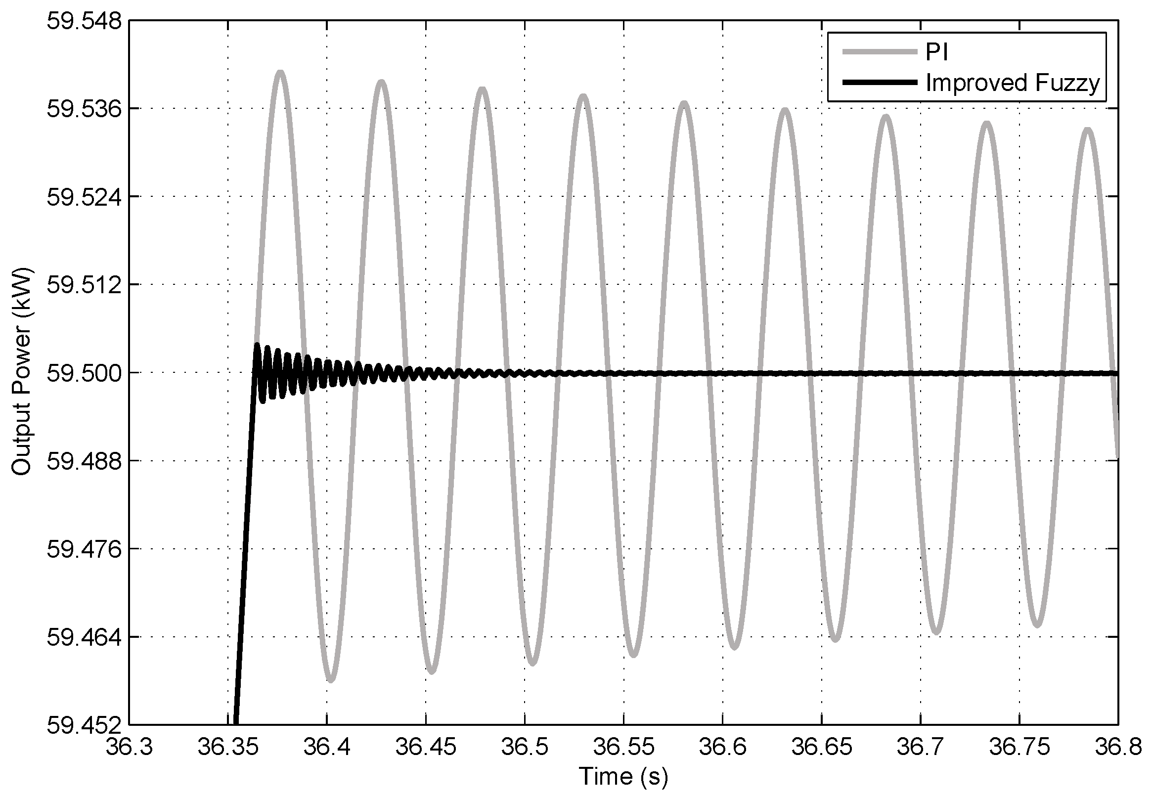
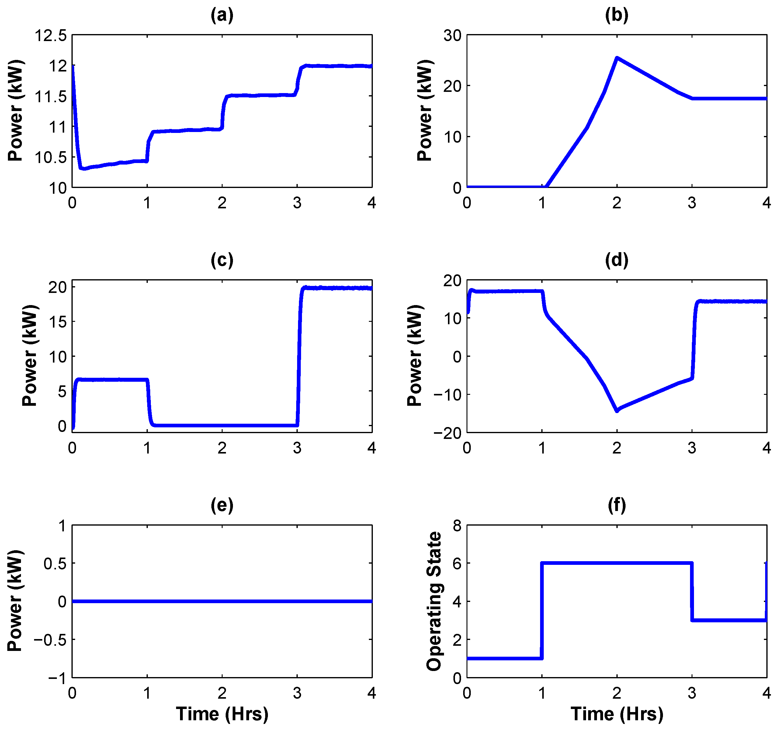
5.1. MATLAB Simulation
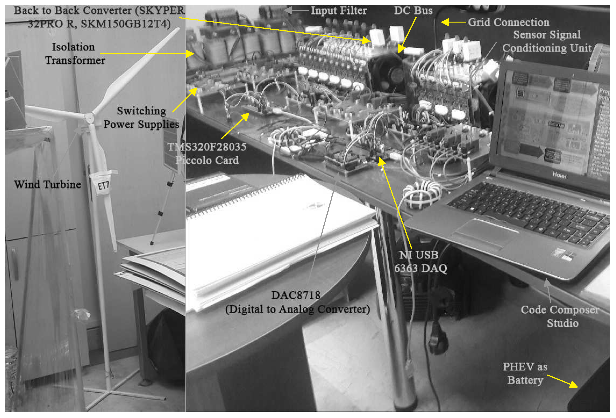
5.2. Experimental Verification
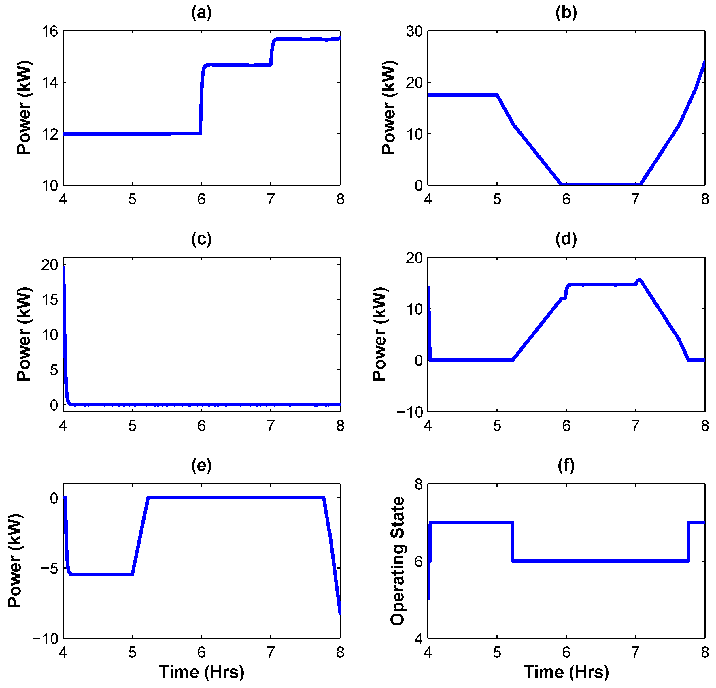
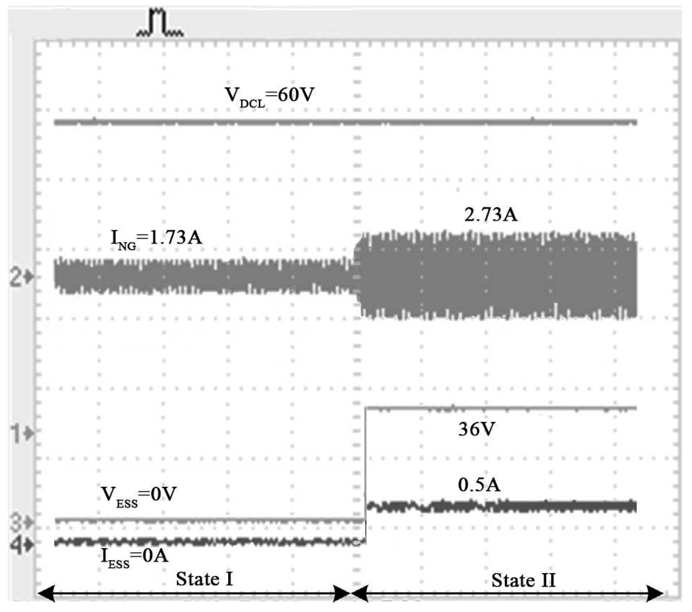
5.2.1. Experimental Results for States I–II
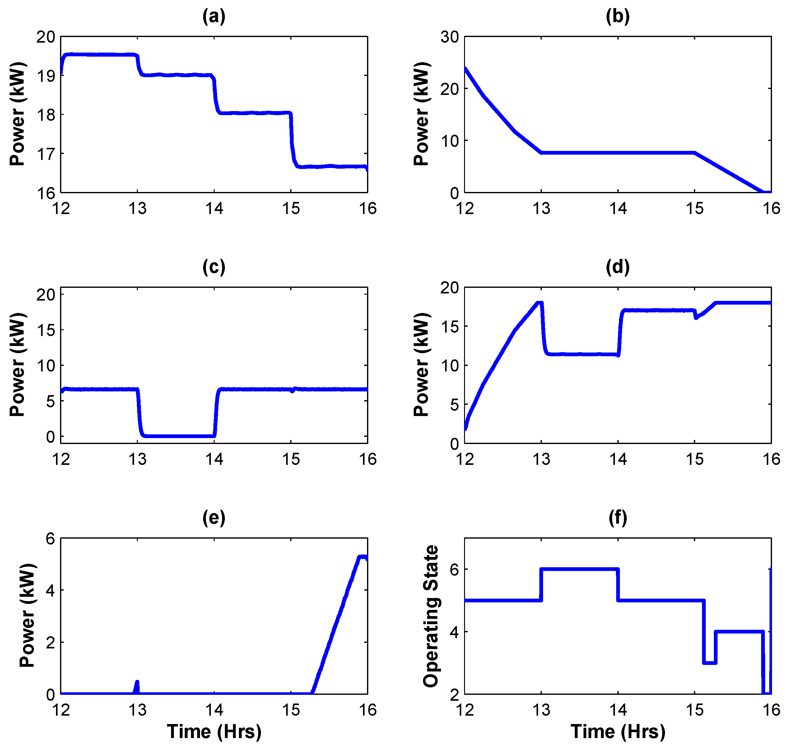
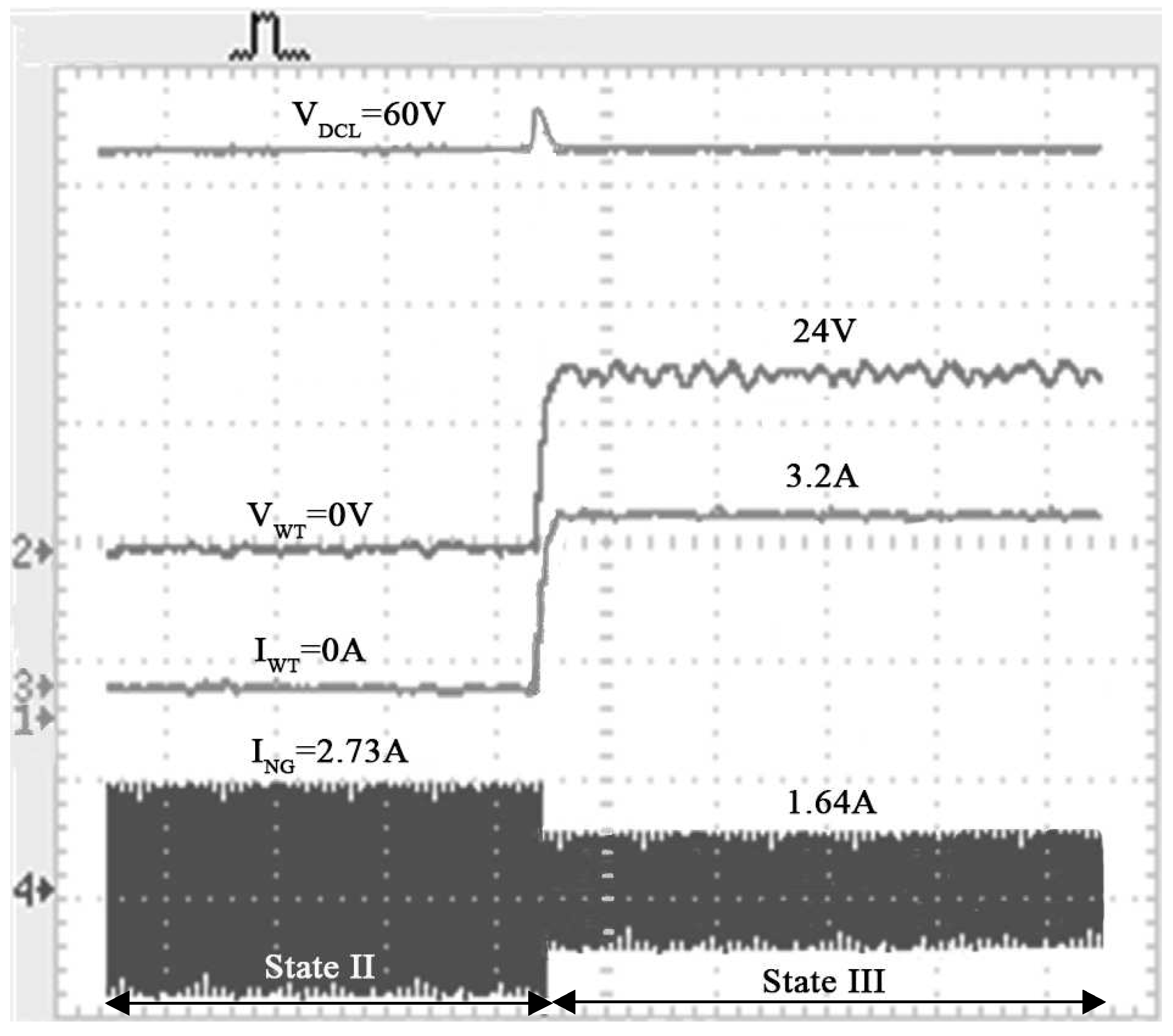
5.2.2. Experimental Results for State II–III
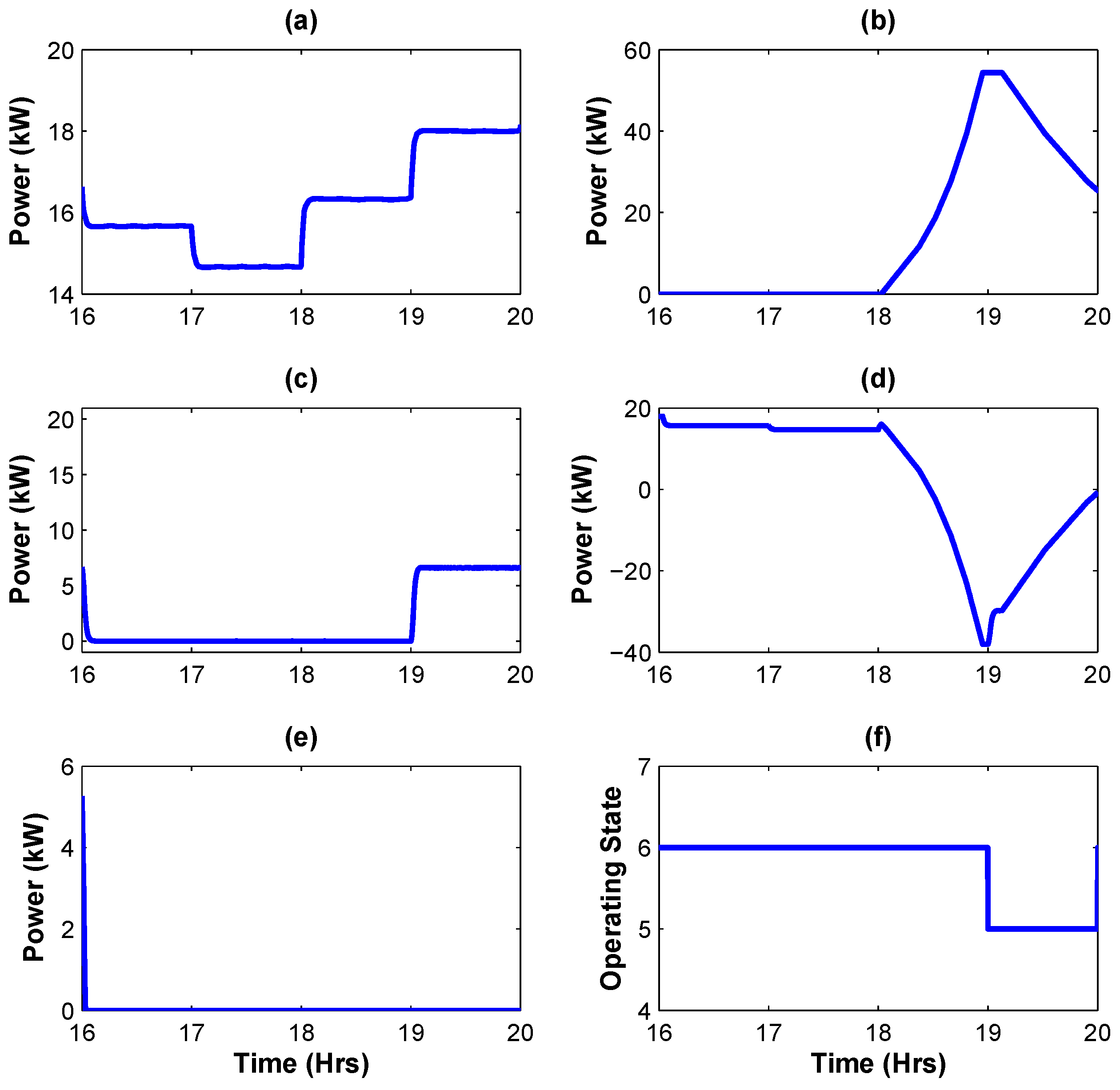
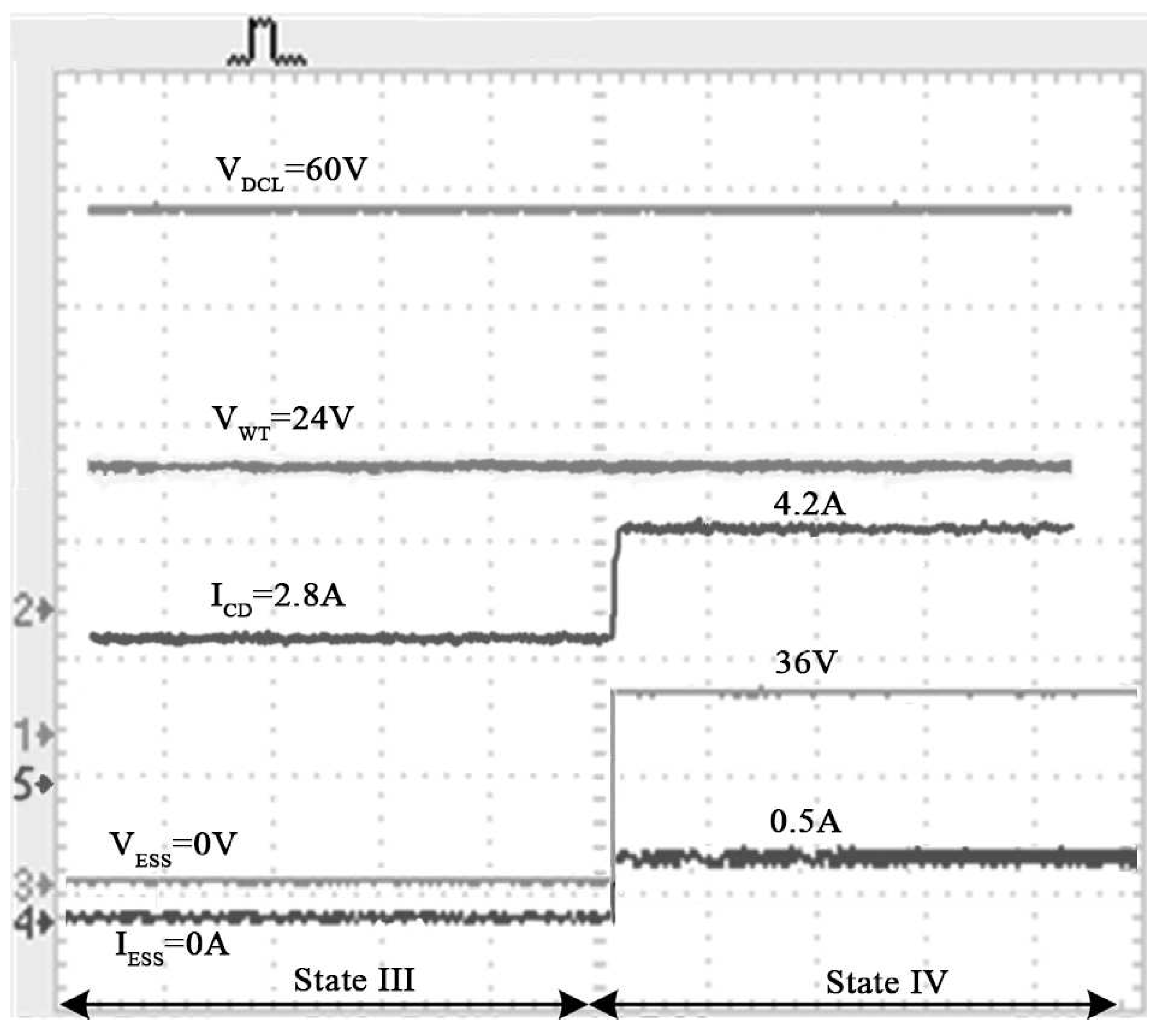
5.2.3. Experimental Results for State III–IV
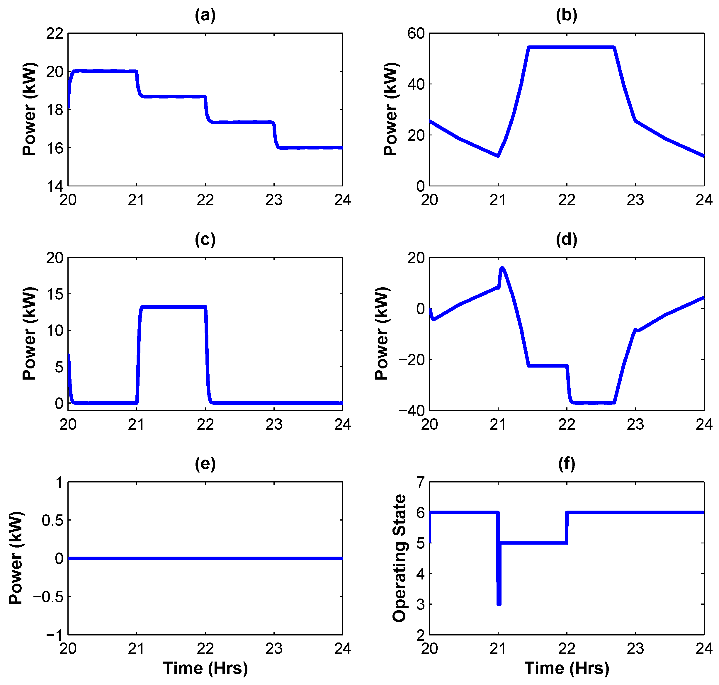
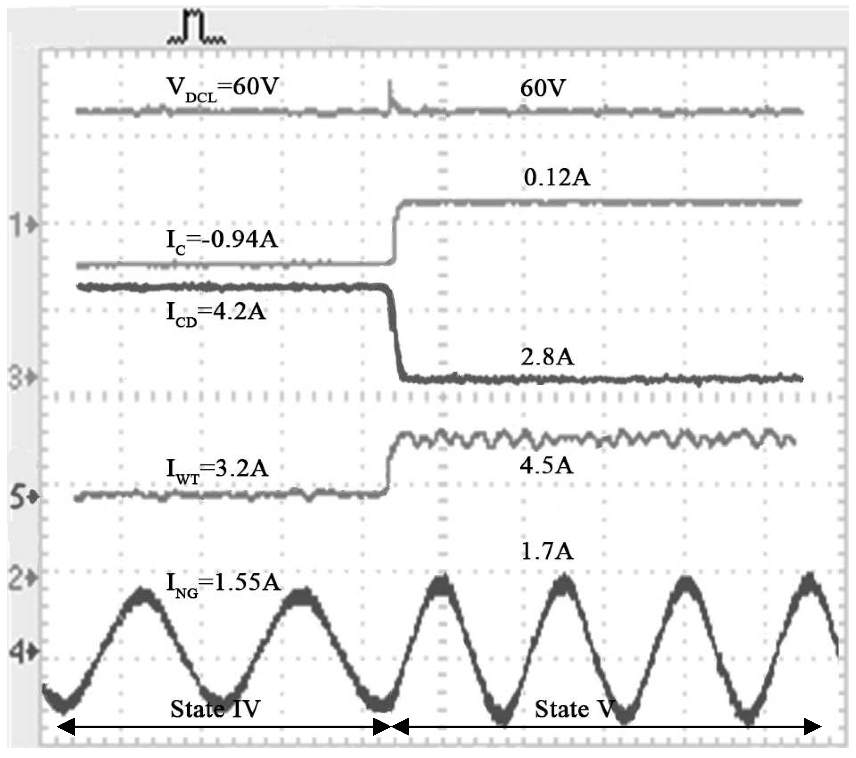
5.2.4. Experimental Results for State IV–V
5.2.5. Experimental Results for State V–VI
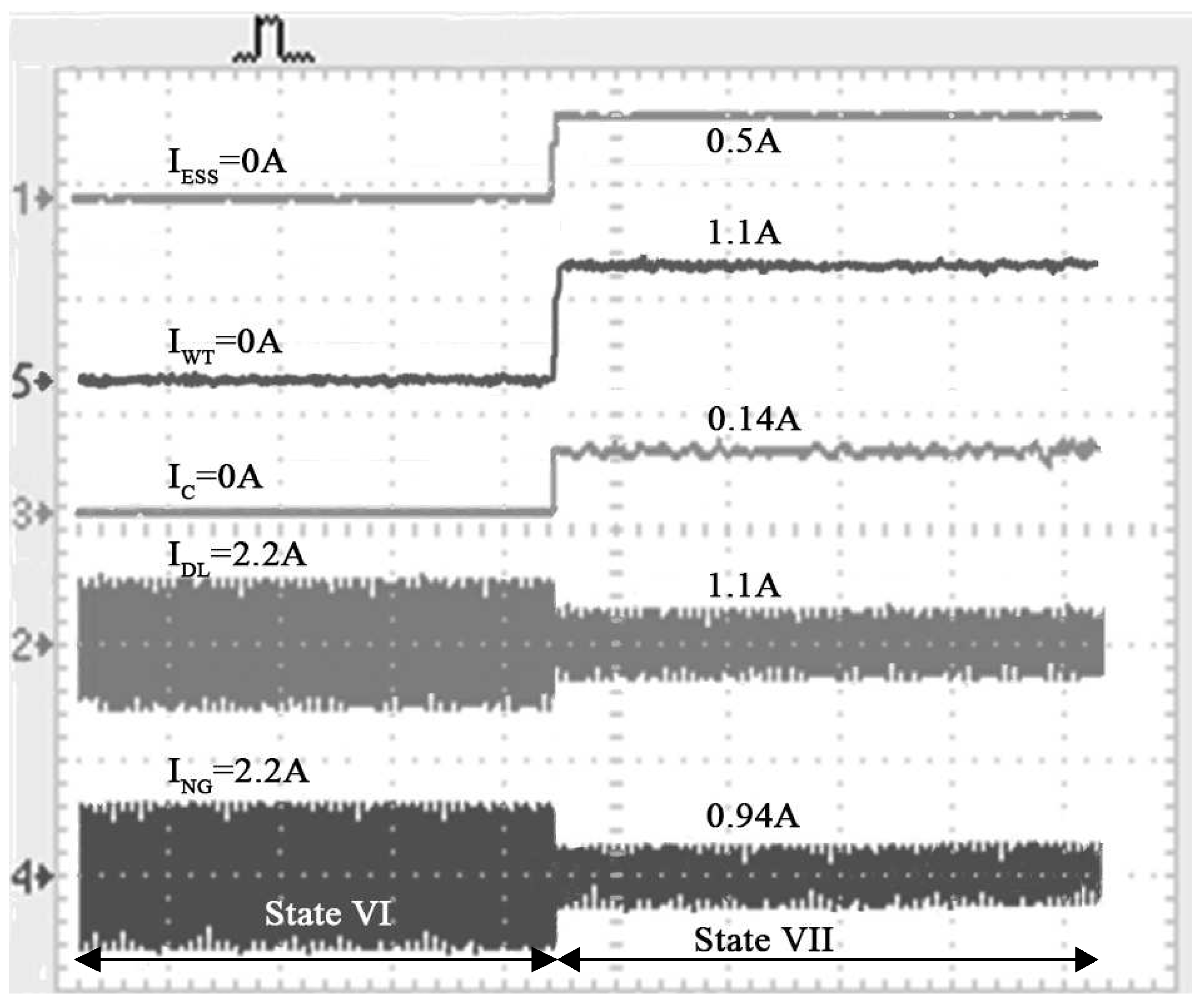
5.2.6. Experimental Results for State VI–VII
6. Conclusions
Author Contributions
Funding
Acknowledgments
Conflicts of Interest
Abbreviations
| Air density | |
| V | Wind speed |
| R | Rotor radius |
| Power coefficient | |
| Torque coefficient | |
| Pitch angle | |
| Tip-speed ratio | |
| Rotor power | |
| Rotor speed | |
| Stator flux | |
| Rotor flux | |
| Stator winding voltage | |
| Rotor winding voltage | |
| Stator winding currents | |
| Rotor winding currents | |
| Self-inductance of the stator and rotor | |
| Mutual inductance between windings | |
| Resistance of the stator and rotor | |
| Frequency of the grid | |
| p | Number of pole pairs |
| Cut-in wind speed | |
| Cut-off wind speed | |
| Rated wind speed | |
| Wind turbine output power | |
| Output power of i-th charging dock | |
| Domestic load power consumption |
References
- Das, T.; Aliprantis, D.C. Small-signal stability analysis of power system integrated with PHEVs. In Proceedings of the IEEEEnergy 2030 Conference, Atlanta, GA, USA, 17–18 November 2008; pp. 1–4. [Google Scholar]
- Duvall, M.; Knipping, E.; Alexander, M.; Tonachel, L.; Clark, C. Environmental assessment of plug-in hybrid electric vehicles. EPRI July 2007, 1, 1–56. [Google Scholar]
- Adams, R.B. Analysis of Spread Moorings By Dimensionless Functions. In Proceedings of the Offshore Technology Conference, Houston, TX, USA, 18–21 May 1969; Volume 2, pp. 77–88. [Google Scholar] [CrossRef]
- Saberbari, E.; Saboori, H. Evaluating PHEV impacts on domestic distribution grid in terms of power losses and voltage drop. In Proceedings of the 2014 19th Conference on Electrical Power Distribution Networks (EPDC), Tehran, Iran, 6–7 May 2014; pp. 52–58. [Google Scholar]
- Goli, P.; Shireen, W. PV Integrated Smart Charging of PHEVs Based on DC Link Voltage Sensing. IEEE Trans. Smart Grid 2014, 5, 1421–1428. [Google Scholar] [CrossRef]
- Preetham, G.; Shireen, W. Photovoltaic charging station for plug-in hybrid electric vehicles in a smart grid environment. In Proceedings of the 2012 IEEE PES Innovative Smart Grid Technologies (ISGT), Washington, DC, USA, 16–20 January 2012; pp. 1–8. [Google Scholar]
- Zhao, J.; Kucuksari, S.; Mazhari, E.; Son, Y.J. Integrated analysis of high-penetration PV and PHEV with energy storage and demand response. Appl. Energy 2013, 112, 35–51. [Google Scholar] [CrossRef]
- Nagarajan, A.; Shireen, W. Grid connected residential photovoltaic energy systems with Plug-In Hybrid electric Vehicles (PHEV) as energy storage. In Proceedings of the IEEE PES General Meeting, Providence, RI, USA, 25–29 July 2010; pp. 1–5. [Google Scholar]
- Green, R.C.; Wang, L.; Alam, M. The impact of plug-in hybrid electric vehicles on distribution networks: A review and outlook. Renew. Sustain. Energy Rev. 2011, 15, 544–553. [Google Scholar] [CrossRef]
- Shao, S.; Pipattanasomporn, M.; Rahman, S. Challenges of PHEV penetration to the residential distribution network. In Proceedings of the 2009 IEEE Power & Energy Society General Meeting, Calgary, AB, Canada, 26–30 July 2009; pp. 1–8. [Google Scholar]
- Rutherford, M.J.; Yousefzadeh, V. The impact of electric vehicle battery charging on distribution transformers. In Proceedings of the 2011 Twenty-Sixth Annual IEEE, Applied Power Electronics Conference and Exposition (APEC), Fort Worth, TX, USA, 6–11 March 2011; pp. 396–400. [Google Scholar]
- Erol-Kantarci, M.; Mouftah, H.T. Management of PHEV batteries in the smart grid: Towards a cyber-physical power infrastructure. In Proceedings of the 2011 IEEE 7th International Wireless Communications and Mobile Computing Conference (IWCMC), Istanbul, Turkey, 4–8 July 2011; pp. 795–800. [Google Scholar]
- Heydt, G. The Impact of Electric Vehicle Deployment on Load Management Straregies. IEEE Trans. Power Appar. Syst. 1983, PAS-102, 1253–1259. [Google Scholar] [CrossRef]
- Giges, N.S. Wind-Powered Charging Stations Coming Soon. Available online: https://www.asme.org/engineering-topics/articles/renewable-energy/wind-powered-charging-stations-coming-soon (accessed on 3 March 2019).
- Ghanbarzadeh, T.; Baboli, P.T.; Rostami, M.; Moghaddam, M.P.; Sheikh-El-Eslami, M.K. Wind farm power management by high penetration of PHEV. In Proceedings of the 2011 IEEE Power and Energy Society General Meeting, Detroit, MI, USA, USA, 24–29 July 2011; pp. 1–5. [Google Scholar]
- Short, W.; Denholm, P. A Preliminary Assessment of Plug-in Hybrid Electric Vehicles on Wind Energy Markets; National Renewable Energy Laboratory: Lakewood, CO, USA, 2006.
- Goli, P.; Shireen, W. Wind powered smart charging facility for PHEVs. In Proceedings of the 2014 IEEE Energy Conversion Congress and Exposition (ECCE), Pittsburgh, PA, USA, 14–18 September 2014; pp. 1986–1991. [Google Scholar]
- Dallinger, D.; Gerda, S.; Wietschel, M. Integration of intermittent renewable power supply using grid-connected vehicles—A 2030 case study for California and Germany. Appl. Energy 2013, 104, 666–682. [Google Scholar] [CrossRef]
- Hassan, S.Z.; Kamal, T.; Mumtaz, S.; Khan, L. A Road to Wind Based PHEVs Smart Charging Station. In Proceedings of the 2015 13th International Conference on Frontiers of Information Technology (FIT), Islamabad, Pakistan, 14–16 December 2015; pp. 41–46. [Google Scholar] [CrossRef]
- Sagosen, Ø.; Molinas, M. Large scale regional adoption of electric vehicles in Norway and the potential for using wind power as source. In Proceedings of the 2013 International Conference on Clean Electrical Power (ICCEP), Alghero, Italy, 11–13 June 2013; pp. 189–196. [Google Scholar]
- Mets, K.; De Turck, F.; Develder, C. Distributed smart charging of electric vehicles for balancing wind energy. In Proceedings of the 2012 IEEE Third International Conference on Smart Grid Communications (SmartGridComm), Tainan, Taiwan, 5–8 November 2012; pp. 133–138. [Google Scholar]
- Kamal, T. Adaptive Control of Fuel Cell and Design of Power Management System (PMS) for PHEVs/EVs Charging Station in a Hybrid Power System. Ph.D. Thesis, COMSATS Institute of Information Technology Abbottabad-Pakistan, Abbottabad, Pakistan, 2014. [Google Scholar]
- The 2014 Accord Plug-In. 2014. Available online: https://www.cnet.com/roadshow/reviews/2014-honda-accord-plug-in-hybrid-review/ (accessed on 3 March 2019).
- IEEE Standard for Interconnecting Distributed Resources with Electric Power Systems. Available online: https://ieeexplore.ieee.org/document/1225051 (accessed on 3 March 2019).


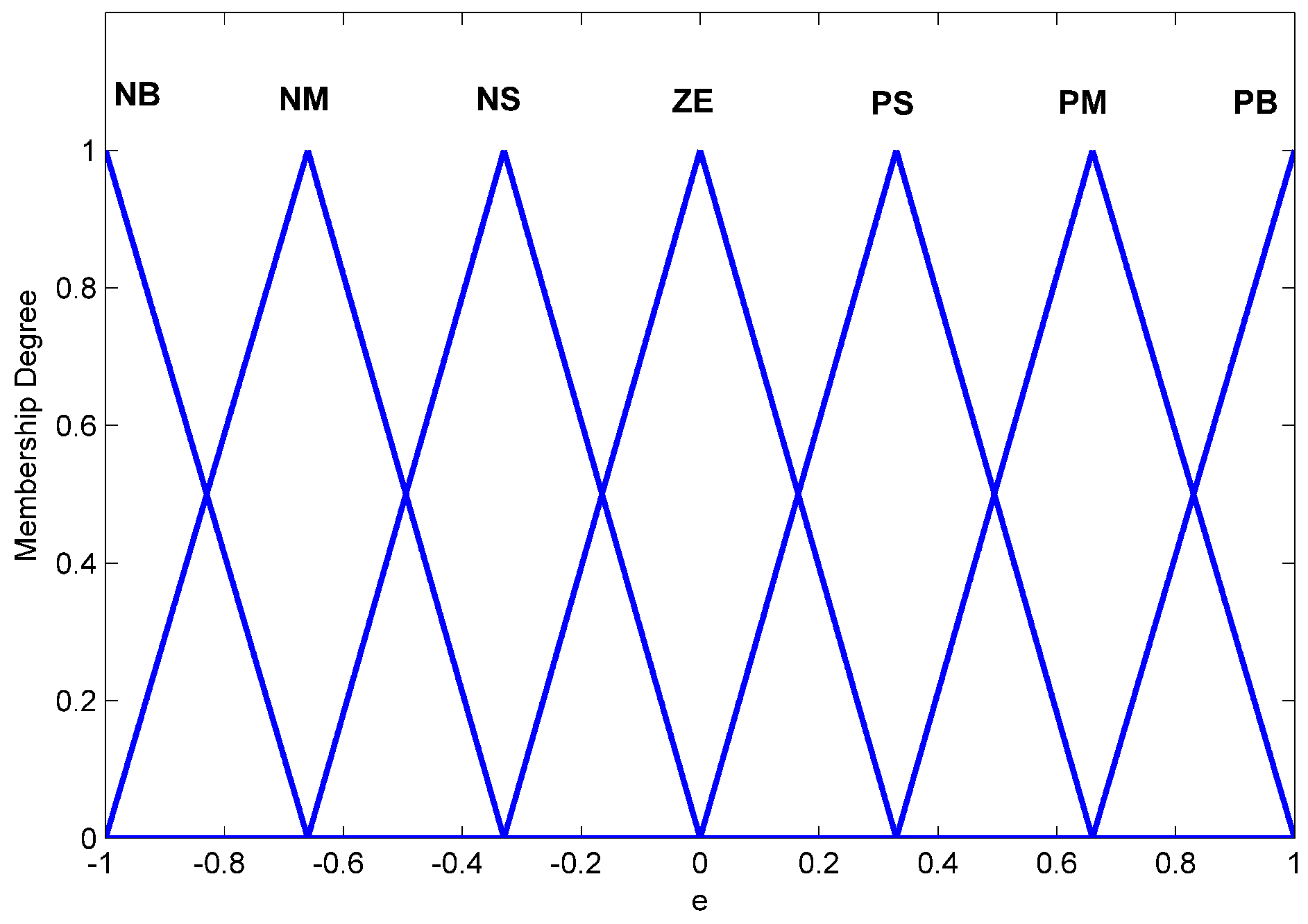
| e | |||||||
|---|---|---|---|---|---|---|---|
| NB | NM | NS | ZE | PS | PM | PB | |
| NB | PB | PM | PS | ZE | PB | PB | PB |
| NM | PM | PM | PS | ZE | PM | PM | PM |
| NS | PS | PS | PS | ZE | PS | PS | PS |
| ZE | ZE | ZE | ZE | ZE | NS | NS | ZE |
| PS | NS | NS | NB | NB | NS | NS | NS |
| PM | NM | NB | NB | NB | NM | NM | NM |
| PB | NB | NB | NB | NB | NB | NB | NB |
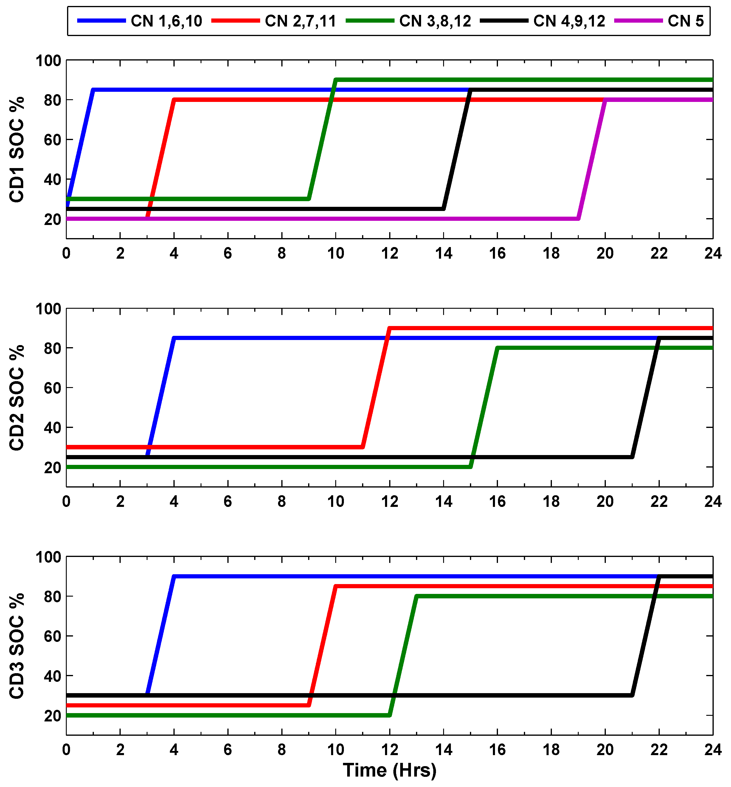
| CD No | Car No | Min SOC | Max SOC | Charging Time (H) | |
|---|---|---|---|---|---|
| (% age) | (% age) | Start | End | ||
| 1 | 1 | 25 | 85 | 0 | 1 |
| 1 | 2 | 20 | 80 | 3 | 4 |
| 1 | 3 | 30 | 90 | 9 | 10 |
| 1 | 4 | 25 | 85 | 14 | 15 |
| 1 | 5 | 20 | 80 | 19 | 20 |
| 2 | 6 | 25 | 85 | 3 | 4 |
| 2 | 7 | 30 | 90 | 11 | 12 |
| 2 | 8 | 20 | 80 | 15 | 16 |
| 2 | 9 | 25 | 85 | 21 | 22 |
| 3 | 10 | 30 | 90 | 3 | 4 |
| 3 | 11 | 25 | 85 | 9 | 10 |
| 3 | 12 | 20 | 80 | 12 | 13 |
| 3 | 13 | 30 | 90 | 21 | 22 |
| Wind Turbine | |
|---|---|
| Type | 300STK2M |
| Rated speed | 800 rpm |
| Output voltage at rated speed | 258 V |
| Cut-off wind speed | 12 m/s |
| Rated power | 8.5 kW |
| National Grid/RL | |
| Phase voltage | 11 kV |
| Operating frequency | 50 Hz |
| Rated power | 10 MVA |
| X/R ration | 5 |
| RL power factor | 0.8 |
| ESS | |
| Type | CINCO FM/BB12100T |
| Capacity | 50 Ah |
| Single module voltage | 12 V |
| Series connected modules | 34 |
| Rated voltage | 12 × 34 ≈ 400 V |
| PHEV Battery | |
| Company name | Honda |
| Vehicle name | Accord |
| Battery capacity | 6.6 kWh |
| Rated voltage | 300 V |
| Fast charging time | 1 H |
| DC/DC Buck Boost Converter (ESS) | ||
|---|---|---|
| Model | NCP1136 | |
| Parameter | Representation | Values |
| Rated voltage | 10/700 V | |
| PID gains () | 1.3, 1.2, 1.1 | |
| Proportional gain () | 1.5, 1.2, 1.3 | |
| Converter capacitance | 2200 F | |
| Converter inductance | 1 mH | |
| f | Rated switching frequency | 10 kHz |
| DC/DC Boost Converter | ||
| Model | MC33363ADWG | |
| Parameter | Representation | Values |
| Rated voltage | 10/700 V | |
| Proportional gain | 0.0006 | |
| integral gain | 0.12 | |
| f | Rated switching frequency | 10 kHz |
| Converter capacitance | 4700 F | |
| Converter inductance | 0.6 mH | |
| DC/DC Buck Converter (CDs) | ||
| Model | NCP1142 | |
| Parameter | Representation | Values |
| Rated voltage | 10/700 V | |
| PID gains () | 1.22, 1.12, 1.31 | |
| Proportional gain () | 1.52, 1.2, 1.32 | |
| Converter capacitance | 3000 F | |
| Converter inductance | 0.8 mH | |
| f | Rated switching frequency | 10 kHz |
| DC/AC Main Converter | ||
| Model | CHZIRI-2VF | |
| Parameter | Representation | Values |
| Rated power | 100 kW | |
| Rated voltage | 220/440 V | |
| Carrier frequency | 10 kHz | |
| Snubber capacitance | 10 F | |
| Snubber resistance | 10 k | |
| L | Inductance L-filter | 2.6 H |
| Component | Rated Voltage | Maximum Current |
|---|---|---|
| PHEVs (each) | 9 V | 1.2 A |
| Wind System | 24 V | 4.5 A |
| ESS | 36 V | 0.5 A |
| DC Link | 60 V | 2.2 A |
| Domestic Load | 220 V (AC) | 1.8 A (RMS) |
| National Grid | 220 V (AC) | 2.73 A (RMS) |
© 2019 by the authors. Licensee MDPI, Basel, Switzerland. This article is an open access article distributed under the terms and conditions of the Creative Commons Attribution (CC BY) license (http://creativecommons.org/licenses/by/4.0/).
Share and Cite
Hassan, S.Z.; Kamal, T.; Riaz, M.H.; Shah, S.A.H.; Ali, H.G.; Riaz, M.T.; Sarmad, M.; Zahoor, A.; Khan, M.A.; Miqueleiz, J.P. Intelligent Control of Wind-Assisted PHEVs Smart Charging Station. Energies 2019, 12, 909. https://doi.org/10.3390/en12050909
Hassan SZ, Kamal T, Riaz MH, Shah SAH, Ali HG, Riaz MT, Sarmad M, Zahoor A, Khan MA, Miqueleiz JP. Intelligent Control of Wind-Assisted PHEVs Smart Charging Station. Energies. 2019; 12(5):909. https://doi.org/10.3390/en12050909
Chicago/Turabian StyleHassan, Syed Zulqadar, Tariq Kamal, Muhammad Hussnain Riaz, Syed Aamir Hussain Shah, Hina Gohar Ali, Muhammad Tanveer Riaz, Muhammad Sarmad, Amir Zahoor, Muhammad Abbas Khan, and Julio Pascual Miqueleiz. 2019. "Intelligent Control of Wind-Assisted PHEVs Smart Charging Station" Energies 12, no. 5: 909. https://doi.org/10.3390/en12050909
APA StyleHassan, S. Z., Kamal, T., Riaz, M. H., Shah, S. A. H., Ali, H. G., Riaz, M. T., Sarmad, M., Zahoor, A., Khan, M. A., & Miqueleiz, J. P. (2019). Intelligent Control of Wind-Assisted PHEVs Smart Charging Station. Energies, 12(5), 909. https://doi.org/10.3390/en12050909