Article

The Effect of Wet Compression on a Centrifugal Compressor for a Compressed Air Energy Storage System

1
Institute of Engineering Thermophysics, Chinese Academy of Sciences, Beijing 100190, China
2
University of Chinese Academy of Sciences, Beijing 100049, China
*
Author to whom correspondence should be addressed.
Energies 2019, 12(5), 906; https://doi.org/10.3390/en12050906
Submission received: 24 January 2019 / Revised: 21 February 2019 / Accepted: 5 March 2019 / Published: 8 March 2019
(This article belongs to the Special Issue Computational Fluid Dynamics (CFD) 2018)

Abstract

:
There is an urgent demand to reduce compression power consumption in Compressed Air Energy Storage (CAES) systems. Wet compression has been widely used in gas turbines to reduce compressor power consumption and improve thermal efficiency, but this technology has not been applied yet in the CAES field. In this paper, a centrifugal compressor for CAES was numerically studied to investigate the effect of wet compression on compressor and droplet motion. The results showed that wet compression makes the performance curve shift to a high-pressure ratio/efficiency. Meanwhile, wet compression lowers the stall margin and narrows the stable operation range, and the effect is enhanced with the increase of water injection ratio or the decrease of average droplet diameter. Wet compression can effectively save compressor power consumption during energy storage, and at the designed pressure ratio, the power consumption can be reduced by 1.47% with a water injection ratio of 3% and an average droplet diameter of 5 μm. Influenced by the inertia and secondary flow, the droplets migrate to the impeller pressure and shroud side, thus causing brake loss by impacting on blades. The migration of droplets strengthens with the increase in the average droplet diameter and flow coefficient.

1. Introduction

Since renewable energy sources such as solar and wind energy are unstable and intermittent, developing energy storage is of great importance for the large-scale use of renewable energy [1]. Compressed Air Energy Storage (CAES) has the advantages of a large energy storage capacity, long energy storage period, high efficiency and low investment costs per unit, and it is considered to be one of the most promising large-scale energy storage technologies [2]. A large-scale Compressed Air Energy Storage (LSCAES) system requires its compression sub-system to have a high-pressure ratio, large mass flow, high efficiency and wide operating range. Therefore, there are benefits in reducing the compression power consumption per unit mass for CAES [3].
An LSCAES system usually adopts multi-stage compression and intermediate cooling to reduce power consumption while achieving a high-pressure ratio. The overall compression process is nearly isothermal compression, but each stage of compression is approximately irreversible adiabatic compression. To reduce the single-stage compression power consumption per unit mass, water droplets can be sprayed into the compressor. The evaporation latent heat is used to reduce the outlet temperature, and the compression process is closer to isothermal compression [4,5]. This technology, called wet compression or overspray, has been widely used in gas turbine to reduce the specific compression work and increase the thermal efficiency.
In 1989, wet compression was first implemented in gas turbines [6]. Currently, it has been widely studied and applied in this field (it has now been applied to more than 1,000 gas turbines all over the world) [7,8,9]. However, it has not been industrially applied in CAES systems, and only a few studies have been done on Isothermal Compressed Air Energy Storage systems [10,11,12,13,14,15]. For example, Qin et al. found that the compression efficiency for a liquid piston increases from 71% to 98% with 5% water injection [10,11]. Srivatsa et al. found that the inclusion of droplet in a liquid piston/expander can effectively improve the efficiency-power trade-off at high flow rates and low efficiency cases [14]. Jia et al. tested wet compression in a compression chamber for CAES system and founded that the efficiency improved 5.7% with water injection 0.416 g/cycle [13]. Chen et al developed a novel isobaric adiabatic CAES system based on volatile fluid, which can improve the exergy efficiency by 4% [12]. Nevertheless, wet compression research in the CAES field mainly focused on the volumetric compressor, and the effect of wet compression on rotating compressor in the CAES system requires further investigation.
LSCAES systems typically employ axial or centrifugal compressors or a combination of the two. However, there are more wet compression studies on axial compressors [16,17,18,19], while only few on centrifugal compressors. Abdelwahab developed a one-dimensional performance prediction model for centrifugal compressors’ wet compression, and the results showed that wet compression shifts the performance curve towards a higher pressure ratio and larger flow rate [20]. The Hitachi company tested the wet compression performance of a small gas turbine with a two-stage centrifugal compressor and found that wet compression increased the pressure ratio and flow rate and augmented the generated power [21]. The Bakken team in the Norwegian University of Science and Technology conducted a series of wet compression experiments on a single-stage centrifugal compressor and found that as the liquid content increases, the pressure ratio rises, and the efficiency declines [22,23,24]. GE Oil & Gas Company conducted a series of wet compression experiments on single-stage and two-stage centrifugal compressors. The results showed that when the liquid mass fraction is ≤ 10%, wet compression improves the pressure ratio, but the results are in contrast when the liquid mass fraction is > 10%. Wet compression reduces the choke flow and narrows the performance curve [25,26,27].
At present, in terms of centrifugal compressors, wet compression research mainly focuses on the performance change (and has not reached consensus). Moreover, research on the effects of the flow field and droplet motion has been insufficient (with a dearth of work, such as Surendran [28], Halbe [29], etc.). Therefore, in this paper, the wet compression on a centrifugal compressor for a LSCAES system is numerically simulated. The influence and mechanism of wet compression on centrifugal compressor performance and the droplet motion pattern are studied.

2. Research Object

The research object is a large flow coefficient centrifugal compressor used in an LSCAES system. The designed inlet flow coefficient φ is 0.16, which is defined as equation (1), and the model and the grid are shown in Figure 1. The impeller is an unshrouded impeller with the blade number of 13, and the diffuser is a low solidity vaned diffuser with the vane number of 10. The total inlet pressure is 97000 Pa, and the total inlet temperature is 303.15 K.
The computational domain is meshed by ANSYS TurboGrid, and a refined mesh is adopted in the regions near the wall boundaries. The grid numbers of the impeller and diffuser domain are 1.07 × 10⁶ and 0.51 × 10⁶, respectively, for a total of 1.58 × 10⁶. Grid independence is analyzed in Section 3.4:
ϕ = 4 Q 1 π D 2 2 U 2
where Q1 is the inlet volume flow, D2 is the impeller outlet diameter, U2 is the circumferential velocity at the impeller outlet.

3. Numerical Methodology

The steady-state Reynolds Averaged Navier-Storkes equations are solved for the one periodic blade passage computational domain using ANSYS CFX. The continuous phase is modelled using the variable composition mixture model, and the species are dry air and water vapour, respectively, with the vapour mass fraction being zero at the inlet. The turbulence is modelled using the shear stress transport k-ω model, which performs well in adverse-pressure-gradient separation flows. The mixing plane method is used to exchange the rotor-stator interface data. The dispersed phase is modelled using the particle transport model, and its material is water liquid. In this model, the continuous phase is solved using the Eulerian method, and the dispersed phase is solved using the Lagrangian method. The two phases are fully coupled for the mass, momentum and heat transfer.
For dry compression, the values of the total temperature and the total pressure at the inlet boundary are 303.15 K and 97000 Pa, respectively, and the inlet flow direction is axial. The mass flow rate is given at the outlet boundary, and the dry compression performance curve is obtained by varying the mass flow rate. For wet compression, the inlet total temperature and total pressure of the continuous phase are the same as those for dry compression. Meanwhile, the water injection ratio, droplet temperature, droplet velocity and mean diameter are given for the dispersed phase. The wet compression performance curve is obtained by varying the outlet circumferential-average static pressure. The wall boundary conditions in all cases are adiabatic with no slip. In the study, the operation point with a sudden drop of both the flow coefficient and pressure ratio is regarded as the numerical stall point [30].

3.1. Governing Equations of Dispersed Phase

3.1.1. Motion Equation

In the particle transport model, the forces acting on the droplet include the drag force (FD), the buoyancy force due to gravity (FB), the centrifugal and Coriolis force (FR), the virtual mass force (FVM) and the pressure gradient force (FP) for a rotating reference coordinate. For a single droplet, the motion equation is written as follows:
m p d u p d t = F D + F B + F R + F V M + F P
where mp is the mass of a single droplet, up is the droplet velocity, t is time.
In a high-speed rotating compressor, FB is much smaller than FD and FR, and only when the difference of the interphase density is small FVM and FP are obvious [31]. Therefore, for the present study, the main forces of droplets are FD and FR, and the motion equation is rewritten as follows:
m p d u p d t = F D + F R
FD and FR are respectively as follows:
F D = π 8 C D ρ a d 2 | u u p | ( u u p )
F R = π d 3 ρ p 6 [ 2 Ω × u p Ω × ( Ω × r ) ]
where ρ a is the air density, d is the droplet diameter, u is the air velocity, Ω and r are the angular velocity and position vector in the rotating reference coordinate respectively. CD is the drag coefficient, which is determined by the following empirical correlation:
C D = max ( 24 / R e p ( 1 + 0.15 R e p 0.687 ) , 0.44 )
where Rep is the droplet Reynolds number, which is defined as follows:
R e p = ρ a d | u p u | μ a
where μa is the air dynamic viscosity.

3.1.2. Heat Transfer Equation

The interphase heat transfer between the continuous phase and the dispersed phase includes the convection heat transfer and the phase change heat transfer. It is assumed that the internal temperature of the droplet is uniform, and so the heat transfer of a single droplet can be calculated from the following equation:
m p C w d T p d t = π d λ N u ( T T p ) + d m p d t h f g
where T and Tp are the air and droplet temperature respectively, Cw is the specific heat capacity of the droplet, λ is the air thermal conductivity, hfg is the latent heat of vaporization. Nu is the Nusselt number, which is defined as follows:
N u = 2 + 0.6 R e p 1 / 2 P r 1 / 3
where Pr is the Prandtl number.

3.1.3. Mass Transfer Equation

The liquid evaporation model is employed to model the interphase mass transfer, and it uses two empirical correlations depending on whether the droplet is above or below the boiling point. This is determined by the Antoine equation [32] given below:
log 10 p s a t = A 1 A 2 T + A 3 273.15
where, psat is the Saturation vapor pressure, and A1,2,3 are the Antoine equation parameters.
When the droplet temperature is above the boiling point, the evaporation rate of a single droplet is as follows:
d m p d t = π d λ N u ( T T p ) h f g
When the droplet temperature is below the boiling point, the evaporation rate of a single droplet is as follows:
d m p d t = π d ρ v D v S h M v M log ( 1 x p 1 x )
where ρv is the water vapour density, Dv is the water vapour diffusion coefficient, M and Mv are the air and water vapour molar mass respectively, x and xp are the water vapour and liquid mole fractions respectively. Sh is the Sherwood number which is defined as follows:
S h = 2 + 0.6 R e p 1 / 2 S c 1 / 3
where Sc is the Schmidt number which is defined as follows:
S c = μ a / ( ρ a D a )
where Da is the air diffusion coefficient.

3.2. Water Injection Parameter Settings

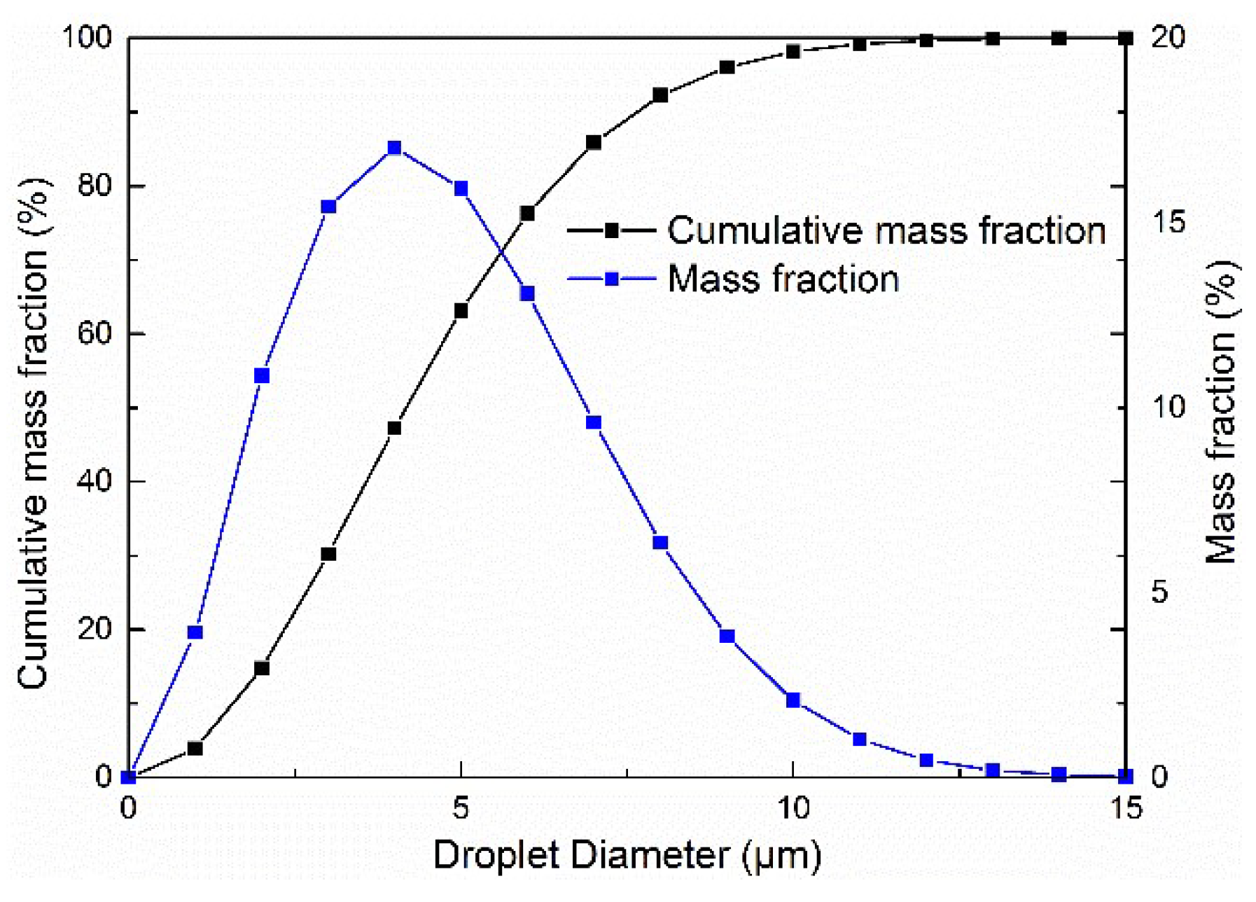
3.2.1. Water Injection Parameters

The research by Chaker et al. [33] showed that droplets of less than 15~20 μm in diameter do not cause compressor blade erosion or blade coating wear. In addition, the average droplet diameter of wet compression is usually in the range of 5~15 μm (the SwirlFlash nozzle from Stork Company has an average droplet diameter of approximately 5 μm [34] and the impaction-pin nozzle from Mee Industries Inc. has an average droplet diameter of approximately 14 μm [35]). Therefore, the average droplet diameters are 5 μm, 10 μm, and 15 μm in this study.
Bhargava et al. [36] pointed out that limited by the compressor loading, surge margin and other factors, the wet compression’s water injection ratio generally does not exceed 2~3%. Moreover, for the cases in this study, the numerical results will diverge when the water injection ratio exceeds 3%, so the water injection ratios are 1%, 2%, and 3%. The water injection mass flow is relative to the designed air mass flow, so the water injection mass flow is equal to the designed air mass flow multiplied by the water injection ratio in this paper.
The initial water injection velocity is set to 100 m/s, and the initial droplet temperature is set to 298.15 K. The water vapour mass fraction at the inlet is set to 0. The initial droplet diameter distribution is assumed to be in accordance with the law of Rosin-Rammler:
R = exp [ ( d / d e ) n ]
where R is the droplet mass fraction above the diameter d, de is the average droplet diameter and n is the droplet diameter distribution parameter.
Referring to the settings of Sun et al. [37], we set n = 2. Figure 2 is the distribution of the droplet diameter when n = 2 and de = 5 μm. The water injection ratio is defined as the ratio of the water mass flow and the air design mass flow at the compressor inlet.

3.2.2. Droplet/Wall Interaction Parameters

The Sommerfeld Collision Model is adopted for droplet-wall collisions. It is assumed that droplets impacting onto the blade will break up into smaller ones and droplets impacting onto other walls will be trapped and removed [37]. Considering the droplet momentum loss, the perpendicular and parallel restitution coefficients are set as 0.5 when droplets impact the rotating blade [38]. To consider the velocity slip effect, a secondary breakup model is needed, so the cascade atomization and breakup model are chosen in the paper.

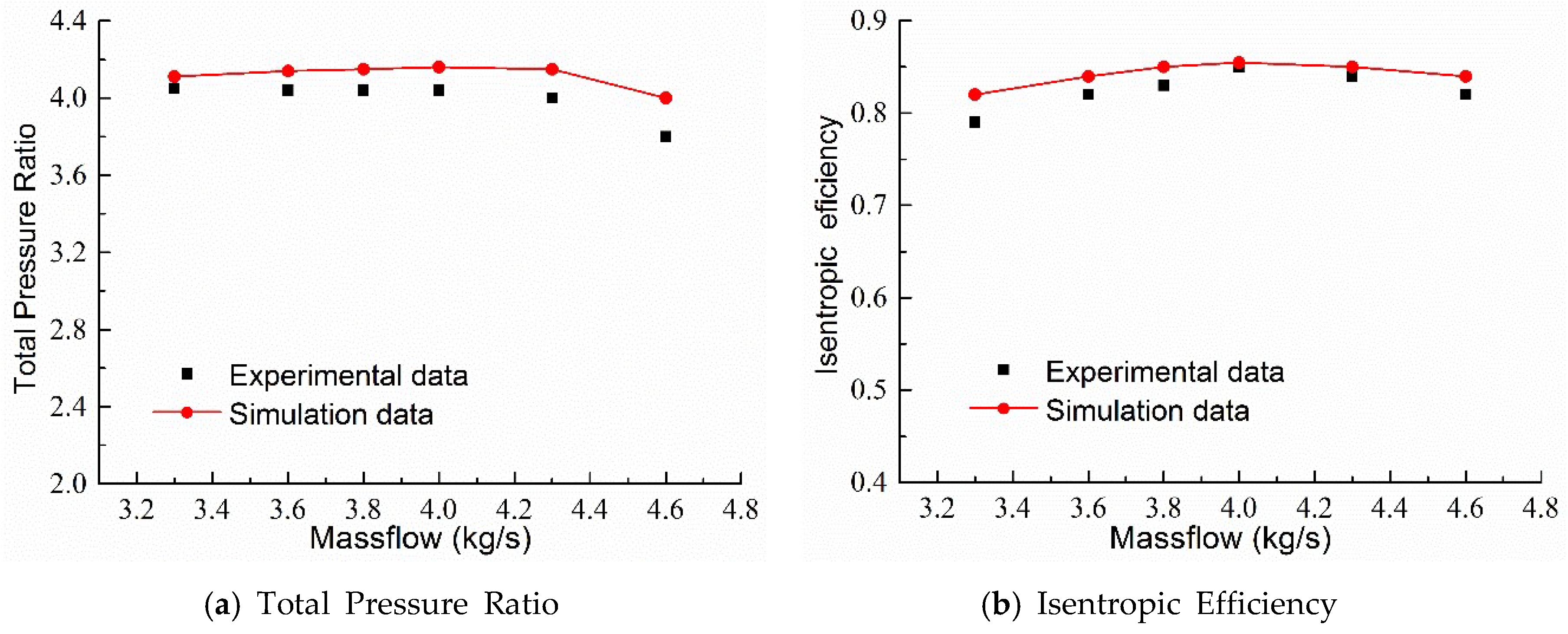
3.3. Numerical Method Validation

The numerical validations of the turbulence model and two-phase flow model are carried out in the paper. A Krain centrifugal impeller was selected to validate the turbulence model. Both this impeller and the research object are subsonic backswept centrifugal impellers. Its designed mass flow rate and pressure ratio are 4 kg/s and 4.7, respectively [39]. The comparisons of the simulation and experiment data are shown in Figure 3. It can be found that the total pressure ratio and isentropic efficiency are in good agreement, demonstrating that the selected turbulence model is suitable for the research object in this paper.
The NACA 64-210 airfoil is chosen to validate the two-phase flow model. The geometry and experimental data are from the literature [40], and the rainfall parameters are from the literature [41]. The comparisons of the simulation and experiment data with rainfall are shown in Figure 4. The average deviations of the lift and drag coefficients between the simulated and experimental data are approximately 6% and 8%, respectively. The relative deviations between rain and no rain are shown in Figure 5 and the simulated and experimental data have the same trend. It is proved that the chosen two-phase flow model is suitable for this research.

3.4. Grid Independence and Data Accuracy Analysis

Grid independence was investigated to exclude the effect of the grid size on the final solution, as shown in Table 1. The isothermal efficiency, pressure ratio, compression work and flow angle at diffuser inlet were chosen as the evaluation indexes, which are the indexes used in this paper. These errors are the relative errors between two adjacent cases.
With an increasing grid number, these indexes change very little, and the error between each case decreases. Compared with case 4, the maximum error is already small enough in case 3. Thus, the grid of case 3 was used for the numerical simulation to reduce the calculation time while ensuring the accuracy.
With the higher precision numerical solution (case 4) as the benchmark solution, the relative errors of isothermal efficiency, pressure ratio, compression work, and flow angle used in this paper (case 3) are 0.06%, 0.12%, 0.07%, and 0.06%, respectively.

4. Results and Discussion

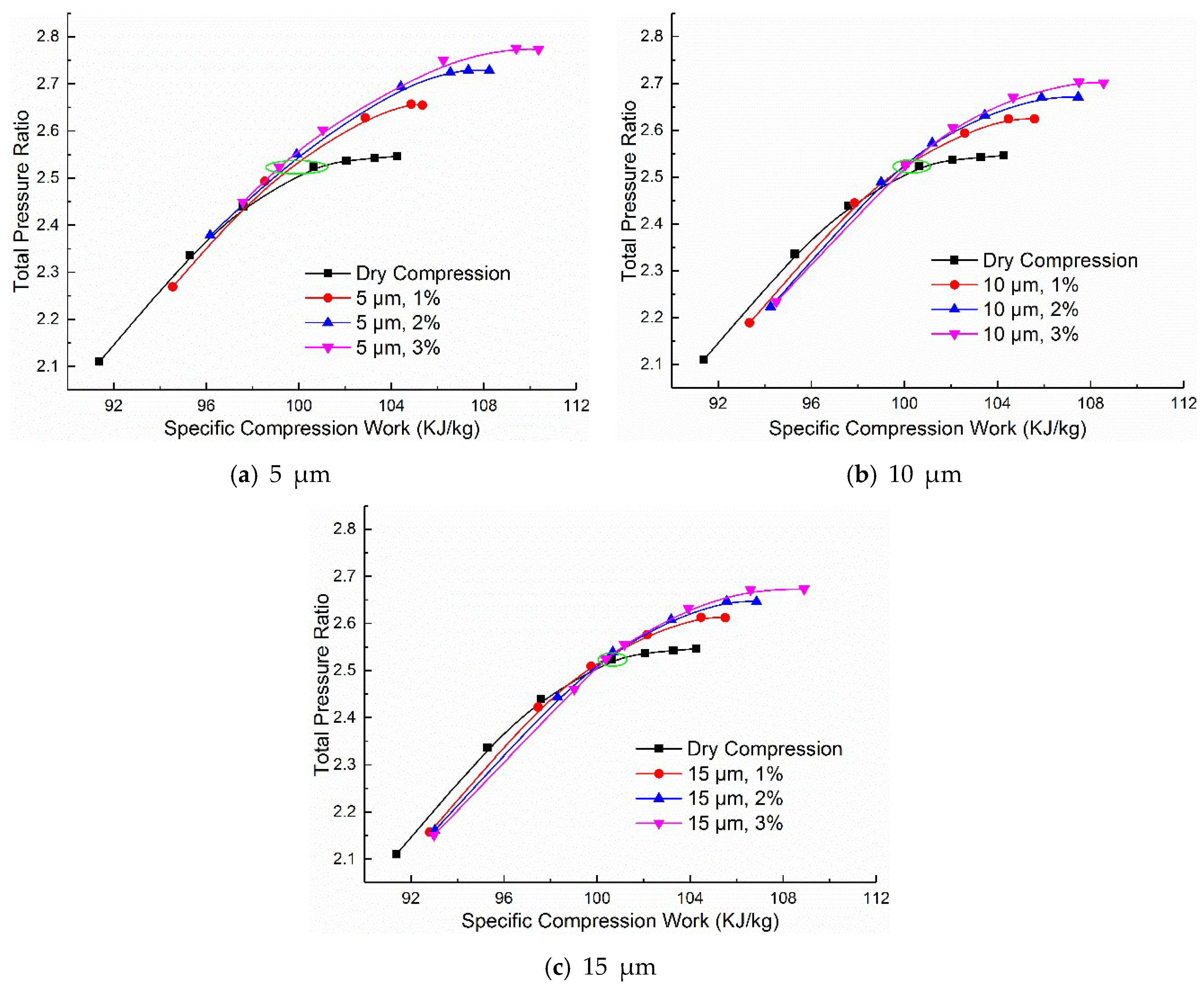
4.1. Overall Performance Analysis

The comparisons of the performance curves between dry compression, different average droplet diameters (5, 10 and 15 μm) and different water injection ratios (1, 2, and 3%) were discussed in this section.
The dry and wet compression performance curves of the total pressure ratio and flow coefficient are shown in Figure 6. The performance curves shift to the higher pressure ratio with the increase in the water injection ratio and the decrease in the average droplet diameter. Meanwhile, the performance curves become narrower due to the increase of the near stall flow rate, which is similar to Abdelwahab’s [20] and Beede’s [42] results.
Compared with dry compression, the total pressure ratio at the design point( at the designed inlet flow coefficient 0.16) respectively increase by 8.95%, 5.78%, and 4.28% when the water injection ratio is 3% and the average droplet diameter is 5, 10 and 15 μm, respectively. Since the wet compression is accompanied by phase change and heat transfer, the gaseous compression is no longer adiabatic. Therefore, the isothermal compression efficiency is chosen as the reference efficiency.
The dry and wet compression performance curves of isothermal efficiency and flow coefficient are shown in Figure 7. With the increase of water injection ratio and the decrease of average droplet diameter, the performance curves shift to the higher efficiency and become steeper. Compared with dry compression, the peak isothermal efficiencies respectively increase by 2.78%, 1.58%, and 0.96% when the water injection ratio is 3% and the average droplet diameter is 5 μm, 10 μm, and 15 μm, respectively. The wet compression isothermal efficiency ηw is calculated as:
η w = w w i w w
where wwi and ww are the isothermal and actual compression work for wet compression, respectively. They are defined as follows:
w w i = ( w a + f w v ) / ( 1 + f )
w w = ω M t / m
where f is the water to air ratio, ω is the rotational speed, Mt is the torque, m is the air mass flow. wa and wv are the isothermal compression work of air and water vapour, respectively. They are defined as follows:
w a = R g a ln ( P R )
w v = R g v ln ( P R )
where Rga is the gas constant of air, Rgv is the gas constant of water vapour, PR is the total pressure ratio.
The dry and wet compression performance curves of the total pressure ratio and specific compression work are shown in Figure 8. Compared with dry compression, wet compression can reduce the specific compression work at the same pressure ratio, or in other words, it can enhance the pressure ratio at the same compression work. Its influence increases with the increase of water injection ratio and the decrease of average droplet diameter. At the designed pressure ratio 2.524, the specific compression works decreases by 1.47%, 0.58%, and 0.25% when the water injection ratio is 3%, and the average droplet diameter is 5 μm, 10 μm, and 15 μm, respectively (The green circle in Figure 8). The last two values above are relatively small. According to the accuracy analysis in Section 3.4, they are close to the accuracy limit of the specific compression work, but this does not affect the validity of the conclusion.
However, wet compression deteriorates the compressor performance and raises the specific work near the choke boundary. The performance deterioration becomes more severe as the average droplet diameter and water injection ratio increase.

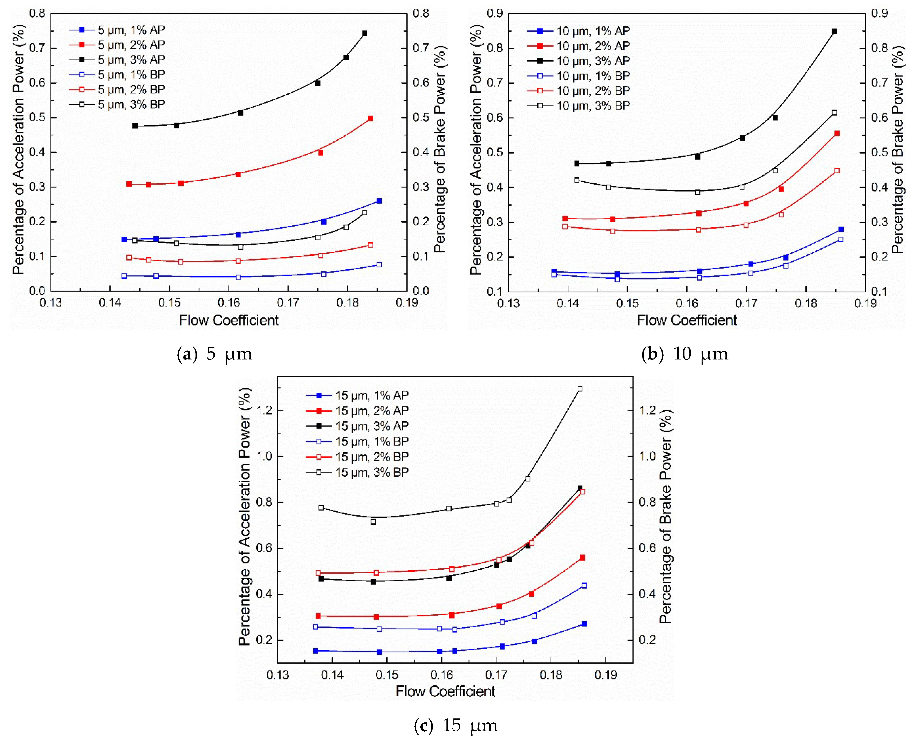
4.2. Analysis of the Work Reduction Mechanism

In [43], White et al. pointed out that “the mechanism for work reduction is essentially the increase in density brought about by cooling”. The effect is readily evaluated from the Gibbs equation:
T d s = d h d p ρ
From the perfect gas expressions, the above equation is rewritten as follows:
d h = T ( d s + R g d p p )
where dh is the specific enthalpy rise, and ds is the entropy increase due to aerodynamic losses.
The droplets’ evaporative cooling lowers the temperature, which reduces the compression work (dh declines). However, the droplets are accelerated by the airflow and collide on the blades, creating additional aerodynamic losses (increases ds) and increasing the compression work. Whether the compression work is reduced depends on the influence of these two factors.
The temperature drop of wet compression depends on the interphase heat transfer. It can be seen from Equation (23) that the heat transfer is proportional to f and 1/d. Figure 9 shows the outlet temperature drop of wet compression (compared to dry compression). The amplitude of the outlet temperature drop strengthens as the water injection ratio increases and the droplet average diameter declines. However, the amplitude falls as the flow coefficient increases, thus indicating that the cooling effect is weakened.
For a certain mass flow of water injection, the interphase heat transfer can be derived from Equation (8):
m l C w d T p d t = 3 m d f d ( λ N u ( T T p ) d ρ p + h f g d d d t )
where ml is the water injection mass flow, md is the designed air mass flow.
Droplets are accelerated by the airflow, thus causing an acceleration loss. The acceleration power Wac (or AP for short) is calculated by the following:
W a c = i = 1 j ( F D + F R ) ( u u p )
where j is the droplet number in the domain, which is calculated as follow:
j = 6 m d f t p π d 3 ρ p
where tp is the droplet residence time in the domain.
Droplets impact on blades, causing brake loss. The brake torque Mtp is calculated by the following:
F p = i = 1 k τ p A p n ^
M t p = F p × r z
where Fp is the brake force due to droplet impacts, rz is the position vector with the rotational axis, τp is the droplet wall stress, k is the number of grid nodes on the blade surface, Ap is the face area of the node, and n ^ is the unit normal to the face.
The brake power (or BP for short) is calculated based on the brake torque. The percentages of acceleration and brake power in total power are shown in Figure 10. The acceleration power enhances with the growth of the water injection ratio, but it basically does not vary with the average droplet diameter. According to Equations (24) and (25), the acceleration power is proportional to f, 1/d, and u-up. Although it reduces 1/d, the increase in the average droplet diameter augments u-up [5], so its effect is almost offset. As the flow coefficient increases, the airflow velocity also improves, thus resulting in a larger slip velocity. Near the choke boundary, the acceleration power has a rapid growth.
The brake power is proportional to the water injection ratio and the average droplet diameter. As the average droplet diameter enlarges, the percentage of brake power gradually exceeds the acceleration power. The brake power grows rapidly near the choke boundary.

4.3. Aerodynamics Stability Analysis

The compressor’s discharge pressure continually rises during the energy storage process in the CAES system, so the stable operating range is one of its consideration factors. From the previous section, we can see that wet compression shifts the near stall point towards the large flow coefficient; thus, the stable operating range of dry and wet compression is analysed. The stall margin of dry and wet compression is shown in Figure 11. With the increase of water injection ratio and the decrease of average droplet diameter, the stall margin declines, and the average droplet diameter has greater influence on it. When applied to the compressor for the CAES system, the effect of wet compression on the stall margin must be considered.
Cumpsty’s definition [44] of the stall margin SM is employed as follows:
S M = [ 1 P R p e a k P R s t a l l m s t a l l m p e a k ] × 100 %
where the subscripts stall and peak indicate the stall and peak points, respectively.

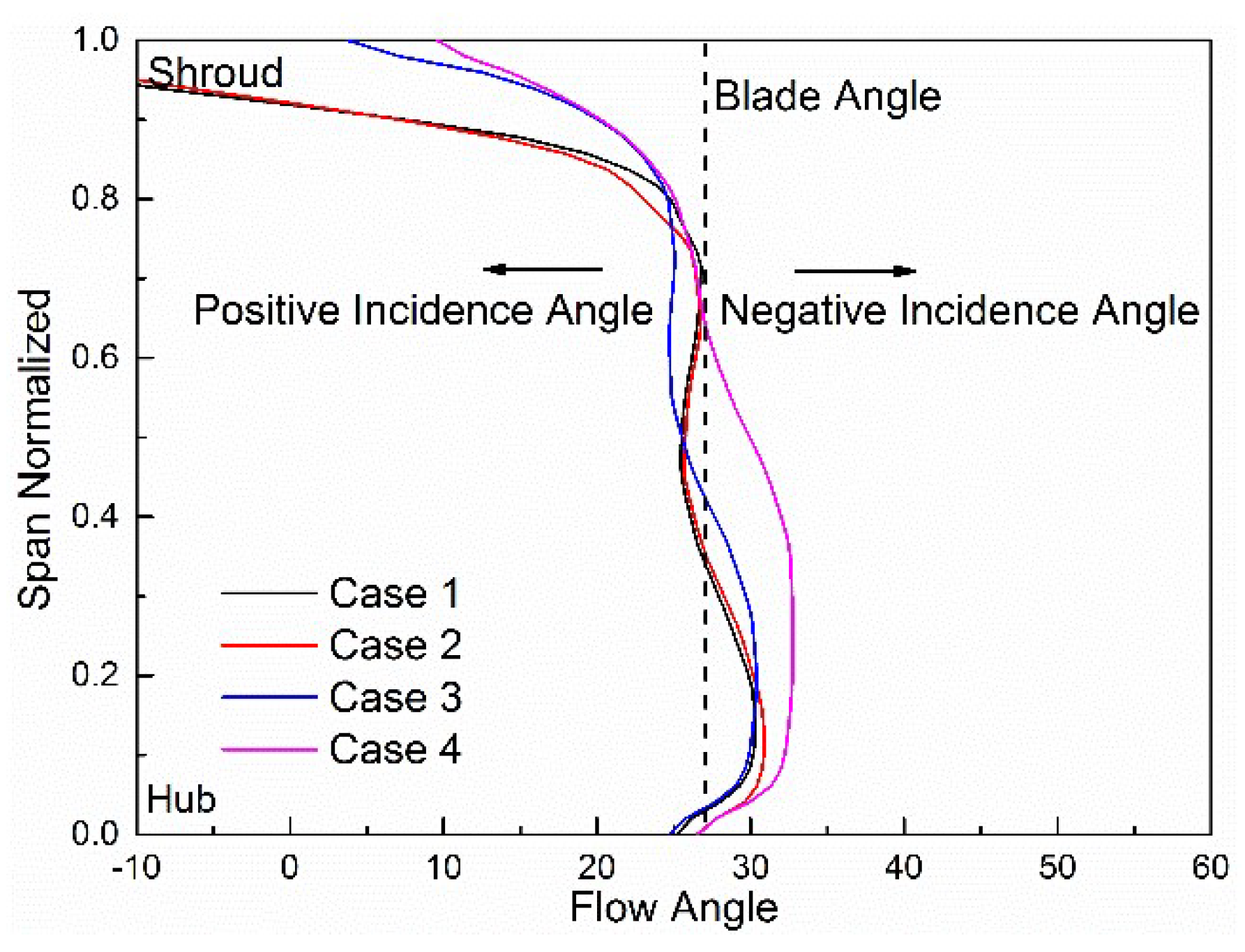
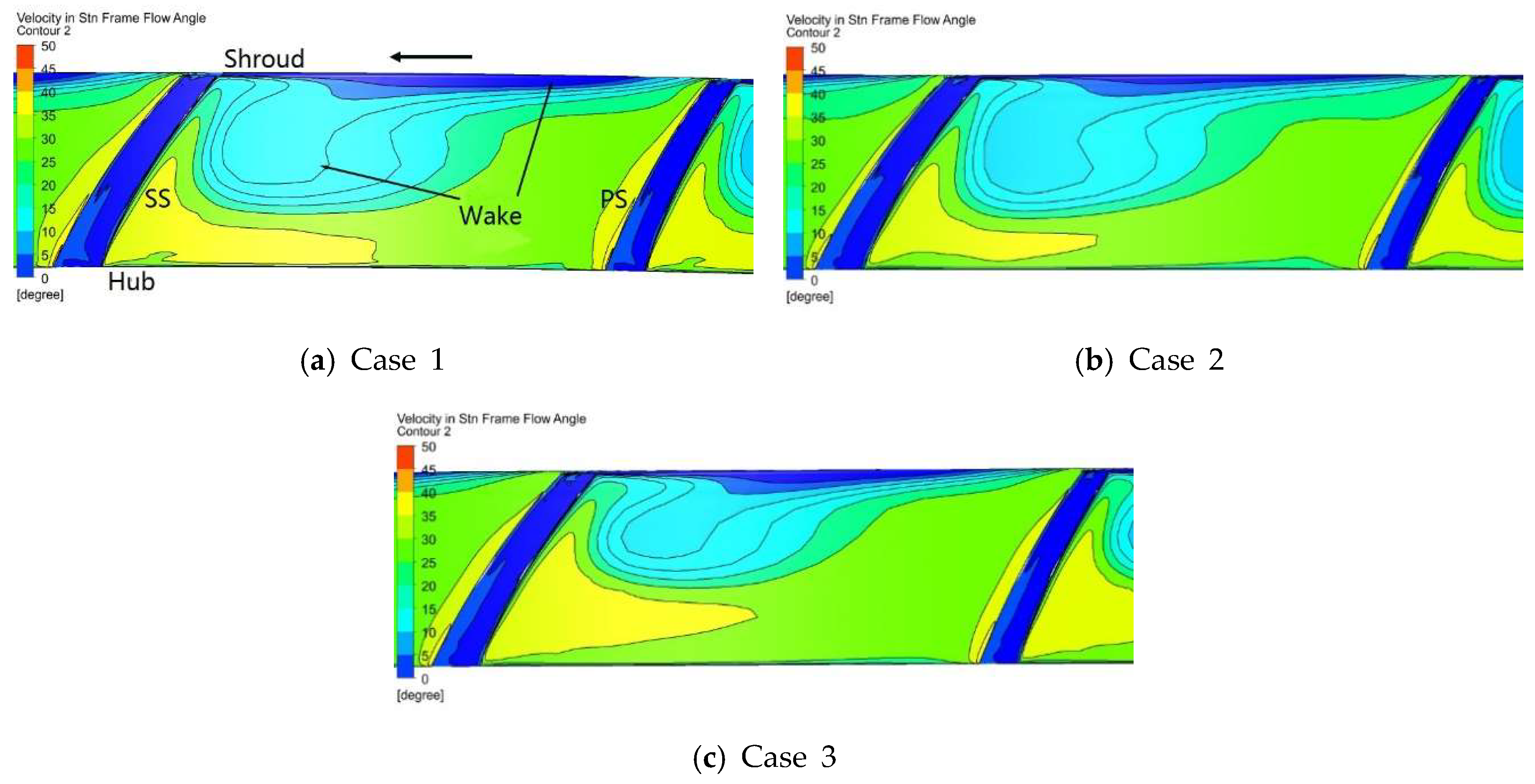
4.3.1. Flow Angle Analysis

To analyse the reasons for the decline of the stall margin, the dry compression near the stall point (flow coefficient 0.13, case 1) and the wet compression near the stall point (water injection ratio 3%, average droplet diameter 10 μm, flow coefficient 0.14, case 2) are chosen. Meanwhile, the dry compression point with the same flow coefficient as the wet compression (flow coefficient 0.14, case 3) and the dry compression design point (flow coefficient 0.16, case 4) are chosen as references.
In the studied centrifugal compressor, the stall occurs first in the diffuser as the flow rate decreases. In wet compression, the evaporative cooling of droplets changes the velocity distribution at the impeller exit to the diffuser inlet, and then affects the diffuser inlet flow angle. The diffuser inlet’s average incidence angle and flow angle distribution are shown in Table 2 and Figure 12, respectively. The studied diffuser has a blade angle of 27°, and the stage and diffuser have good performance when the diffuser inlet’s average incidence angle is −2°~−3° [45,46].
At the dry compression design point, the average incidence angle is −2.1°, and the negative incidence angle is mainly concentrated near the hub side. The average incidence angle is 1.2° at the near stall point of dry compression, and the area of the negative incidence angle is clearly narrowed. The range of the positive incidence angle near the shroud side is significantly enlarged. The average incidence angle is 1.5° at the near stall point of wet compression, and the flow angles between dry and wet compression are very similar. However, at the same flow coefficient, the flow angle of dry compression has not yet reached the stall flow angle, thus indicating that the wet compression causes the diffuser inlet flow angle to reach the stall flow angle earlier.
The total pressure loss contours at the 95% span of the diffuser are shown in Figure 13. At the near stall points (case 1 and case 2), the large range of the positive incidence angle near the shroud side leads to the sharp rise in total pressure loss at the leading edge. Meanwhile, for dry compression at the same flow coefficient (case 3), the stall boundary has not yet been reached, and the total pressure loss is relatively small. At the near stall points (case 1 and case 2), a large flow separation vortex corresponds to the high total pressure loss at the leading edge (as shown in Figure 14), but this separation vortex is relatively small for case 3.

4.3.2. Theoretical Analysis

In this section, a theoretical explanation is given for the premature stall of diffuser. At the same flow coefficient, the impeller outlet pressure of wet compression is higher than that of dry compression, and the outlet temperature of wet compression is lower than that of dry compression. According to the ideal gas equation (29), the outlet density of wet compression is higher than that of dry compression. Therefore, according to the continuity equation (30), the meridional component of the absolute velocity of wet compression is lower than that of dry compression. Meanwhile, the pressure ratio is increased by wet compression, which leads to the augmentation of Euler’s work. According to the Euler equation (31) (the research object is the axial intake), the circumferential component of the absolute velocity of wet compression is higher than that of dry compression.
From the above, for the impeller outlet velocity triangle, at the same flow coefficient, wet compression makes the absolute flow angle α2 decrease. Figure 15a,b show the impeller outlet velocity triangles of wet and dry compression at the same flow coefficient (case 2 and case 3) and at the near stall point (case 1 and case 2), respectively, which verifies the above conclusion. Figure 16 shows the impeller outlet’s absolute air angle distribution, and the decrease of the absolute flow angle α2 shows that the area of the low flow angle expands. That is, the wake area enlarges. Therefore, the wake area in case 2 is the same as case 1 and larger than in case 3.
The air trajectory from the impeller outlet (subscript 2) to the vaned diffuser inlet (subscript 3) is a logarithmic spiral that keeps the flow angle constant. The reduction of the absolute flow angle α2 leads to the decrease in the absolute flow angle α3 and the increase in the incidence angle (i > 0) at the vaned diffuser inlet. When the flow coefficient is less than the design value, i > 0, separation occurs at the diffuser pressure side. Therefore, with the decrease in the flow coefficient, compared to dry compression, wet compression makes the incidence angle reach the critical stall angle at the diffuser inlet earlier:
p = ρ R g T
m = ρ A C 2 m
H = C 2 u U 2
where A is the cross section of the flow channel, H is the Euler work. C, W and U are absolute, relative and circumferential velocities respectively. α and β are the absolute and relative flow angles respectively. Subscripts m and u represent the meridional and circumferential components respectively. Subscripts 1 and 2 represent the impeller inlet and outlet respectively. Subscripts d and w mean the dry and wet compression.

4.4. Droplet Motion Analysis

As shown in Section 4.2, the average droplet diameter significantly influences the brake power, so the droplet motion in the impeller must be analysed. Figure 17 and Figure 18 show the droplet trajectory and the droplet-wall stress on the impeller pressure side, respectively. Due to inertia, droplets migrate to the pressure side, and the inertia is proportional to the droplet diameter [16]. The migration of droplets strengthens with the increase in the average droplet diameter, which enhances the droplet-wall stress. The droplet impingement area mainly concentrates on the leading edge and middle part of the blade. From Figure 18c,d, near the choke boundary, the impingement area significantly enlarges and spreads to the impeller outlet, which causes a rapid growth in braking power.
Figure 19 shows the surface streamlines and the droplet trajectories near the pressure side. Secondary flow occurs on the pressure side with the effects of the centrifugal force and pressure gradient between the pressure and suction side. It causes the droplets near the pressure side to migrate to the shroud side. During the process, droplets collide with the blade, thus leading to brake loss. At the near-choke point, the surface streamlines of the secondary flow shift to the impeller outlet. Accordingly, the droplet movement distance near the pressure side extends, which significantly expands the impingement area.

4.5. Discussion of Wet Compression Applied to CAES System

The CAES system efficiency ηE can be written as follows:
η E = W T W C + W H
where WT is the total output power from the turbine, WC is the total input power to compressor, WH is the total input energy from the external heat source.
For a CAES system, the wet compression could only affect compressor power consumption WC directly. The volume and air storage pressure of the compressed air storage tank are constant, so the compressed air storage mass is also unchanging.
Compared with dry compression, wet compression can reduce the specific compression work at the same pressure ratio except near the choke boundary. For a certain mass of air, this will decrease the compressor power consumption. Its decrease will increase the CAES system efficiency. Therefore, wet compression can significantly benefit the CAES system, but it is not required when the compressor is operating near the choke boundary. In addition, the energy absorbed by water evaporation is not wasted because the water condenses and the energy is recycled in the heat exchanger.

5. Conclusions

In this paper, the centrifugal compressor for a CAES system was numerical simulated, and the influence and mechanism of wet compression on the centrifugal compressor performance and the droplet motion patterns were studied. The following main conclusions are proposed:
(1)
Wet compression shifts the performance curve to a high-pressure ratio/efficiency, which can effectively reduce the compression work. However, the performance curve becomes narrower and steeper. The above effects are enhanced with the increase of water injection ratio and the decrease of average droplet diameter. At the designed pressure ratio, the compression work is reduced by 1.47% with a water injection ratio of 3% and an average droplet diameter of 5 μm.
(2)
Wet compression can effectively save the compression work in the energy storage process of the CAES system, thereby improving the system efficiency, meanwhile it could affect the stable operating range of the compressor.
(3)
The droplets’ evaporative cooling reduces the compression work, while the droplet acceleration and impingement on the blade can increase the compression work. At most operating points, the work reduction due to evaporative cooling exceeds the work increment brought by droplet motion, except the near-choke points.
(4)
Wet compression reduces the stall margin and stable operation range because the evaporative cooling of droplets changes the airflow properties, thus making the incidence angle reach the critical stall angle at the diffuser inlet earlier.
(5)
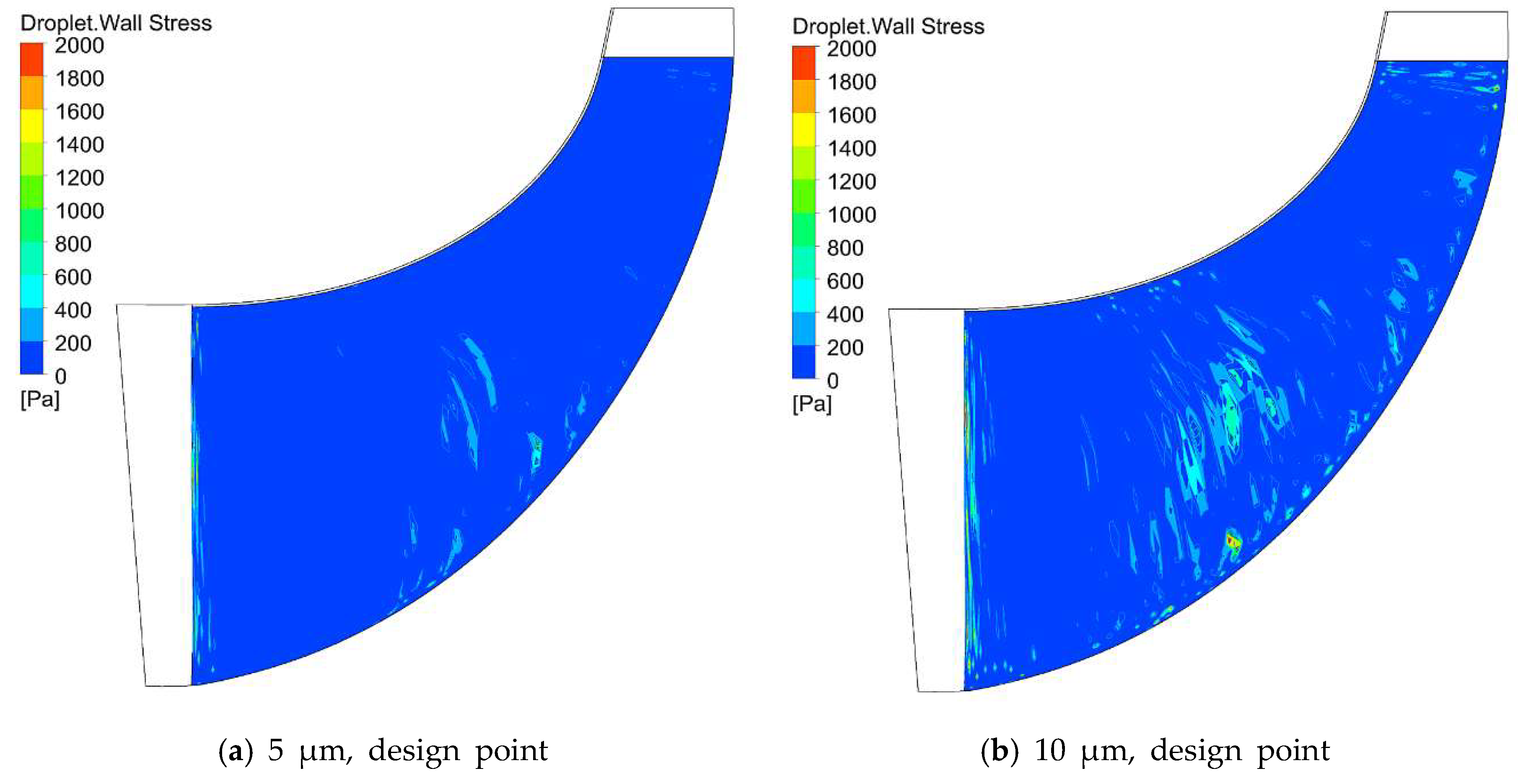
Influenced by the inertia and secondary flow, droplets tend to migrate to the pressure side and shroud the impeller, thus causing brake loss by impacting on blades. The migration of droplets strengthens with the increase of average droplet diameter and flow coefficient.

Author Contributions

Conceptualization, J.S.; Methodology, J.S.; Validation, J.S. and Q.L.; Formal Analysis, J.S. and X.Z.; Data Curation, J.S. and X.Z.; Writing-Original Draft Preparation, J.S.; Writing-Review & Editing, Q.L. and Z.Z.; Supervision, H.C.; Funding acquisition, H.C.

Acknowledgments

The authors acknowledge the support provided by the National Key R&D Plan (2017YFB0903602), the National Natural Science Foundation of China (51522605), the Transformational Technologies for Clean Energy and Demonstration, Strategic Priority Research Program of the Chinses Academy of Sciences (XDA21070200) and the Frontier Science Research Project of CAS (QYZDB-SSW-JSC023).

Conflicts of Interest

The authors declare no conflict of interest.

Nomenclature

ACross section of flow channel (m3)
A1,2,3Antoine equation parameters
ApFace area of the node (m2)
CAbsolute velocity (m/s)
CDDrag coefficient
CwDroplet specific heat capacity (J/(kg·K))
dDroplet diameter (m)
D2Impeller oulet diameter (m)
DaAir diffusion coefficient
deAverage droplet diameter (m)
dhspecific enthalpy rise (J/kg)
dsAerodynamic entropy increase (J/(kg·K))
Dvwater vapour diffusion coefficient
fWater to air ratio
FBBuoyancy force (N)
FDDrag force (N)
FPPressure gradient force (N)
FRCentrifugal and Coriolis force (N)
FVMVirtual mass force (N)
HEuler work (J/kg)
hfgVaporization latent heat (J/kg)
jDroplet number in the domain
kNode number on the blade surface
mAir mass flow (kg/s)
MAir molar mass (kg/mol)
mdDesigned air mass flow (kg/s)
mlWater injection mass flow (kg/s)
mpMass of a single droplet (kg)
MtTorque (N·m)
MtpBrake torque (N·m)
MvWater vapour molar mass (kg/mol)
nDroplet diameter distribution parameter
n ^ Unit normal to the face
NuNusselt number
PrPrandtl number
PRTotal pressure ratio
psatSaturation vapor pressure (Pa)
Q1Inlet volume flow (m3/s)
RDroplet mass fraction above diameter d
rPosition vector
RepDroplet Reynolds number
RgaGas constant of air (J/(kg·K))
RgvGas constant of water vapour (J/(kg·K))
rzPosition vector with the rotational axis
ScSchmidt number
ShSherwood number
SMStall margin (%)
tTime (s)
TTemperature (K)
TpDroplet temperature (K)
tpDroplet residence time in domain (s)
UCircumferential velocity (m/s)
uAir velocity (m/s)
upDroplet velocity (m/s)
WRelative velocity (m/s)
waIsothermal compression work of air (J/kg)
WacAcceleration power (W)
WCTotal input power to compressor (J)
WHTotal input energy from external heat source (J)
WTTotal output power from turbine (J)
wvIsothermal compression work of water vapour (J/kg)
wwActual compression work for wet compression (J/kg)
wwiIsothermal compression work for wet compression (J/kg)
xWater vapour mole fraction
xpWater liquid mole fraction
αAbsolute flow angle (°)
βRelative flow angle (°)
ηECAES system efficiency
ηwWet compression isothermal efficiency
λAir thermal conductivity (W/(m·K))
μaAir dynamic viscosity (Pa·s)
ρaAir density (kg/m3)
ρvWater vapour density (kg/m3)
τpDroplet wall stress (Pa)
φInlet flow coefficient
ΩAngular velocity (rad/s)
ωRotational speed (r/min)

Subscripts

1Impeller inlet
2Impeller outlet
dDry compression
mMeridional component
peakPeak point
stallStall point
uCircumferential component
wWet compression

References

  1. Chen, H.; Cong, T.N.; Yang, W.; Tan, C.; Li, Y.; Ding, Y. Progress in electrical energy storage system: A critical review. Prog. Nat. Sci. 2009, 19, 291–312. [Google Scholar] [CrossRef]
  2. Guo, C.; Xu, Y.J.; Zhang, X.J.; Guo, H.; Zhou, X.Z.; Liu, C.; Qin, W.; Li, W.; Dou, B.L.; Chen, H.S. Performance analysis of compressed air energy storage systems considering dynamic characteristics of compressed air storage. Energy 2017, 135, 876–888. [Google Scholar] [CrossRef]
  3. Guo, H.; Xu, Y.J.; Chen, H.S.; Zhang, X.H.; Qin, W. Corresponding-point methodology for physical energy storage system analysis and application to compressed air energy storage system. Energy 2018, 143, 772–784. [Google Scholar] [CrossRef]
  4. Sureshkumar, R.; Kale, S.R.; Dhar, P.L. Heat and mass transfer processes between a water spray and ambient air—I. Experimental data. Appl. Therm. Eng. 2008, 28, 349–360. [Google Scholar] [CrossRef]
  5. Zheng, Q.; Sun, Y.; Li, S.; Wang, Y. Thermodynamic Analyses of Wet Compression Process in the Compressor of Gas Turbine. In ASME Turbo Expo 2002: Power for Land, Sea, and Air; American Society of Mechanical Engineers: New York, NY, USA, 2002; pp. 487–496. [Google Scholar]
  6. Nolan, J.; Twombly, V. Gas turbine performance improvement direct mixing evaporative cooling system american atlas cogeneration facility rifle, Colorado. In ASME 1990 International Gas Turbine and Aeroengine Congress and Exposition; American Society of Mechanical Engineers: New York, NY, USA, 1990; p. V004T011A021. [Google Scholar]
  7. Bhargava, R.K.; Meher-Homji, C.B.; Chaker, M.A.; Bianchi, M.; Melino, F.; Peretto, A.; Ingistov, S. Gas turbine fogging technology: A state-of-the-art review—Part i: Inlet evaporative fogging—Analytical and experimental aspects. J. Eng. Gas Turbines Power 2006, 129, 443–453. [Google Scholar] [CrossRef]
  8. Yilmazoğlu, M.Z. Effects of a fogging system on a combined cycle performance. Proc. Inst. Mech. Eng. Part A J. Power Energy 2010, 224, 1029–1038. [Google Scholar] [CrossRef]
  9. Zhang, H.; Luo, M.; Pan, X.; Zheng, Q. Numerical analysis of gas turbine inlet fogging nozzle manifold resistance. Proc. Inst. Mech. Eng. Part A J. Power Energy 2016, 230, 63–75. [Google Scholar] [CrossRef]
  10. Qin, C.; Loth, E. Liquid piston compression efficiency with droplet heat transfer. Appl. Energy 2014, 114, 539–550. [Google Scholar] [CrossRef]
  11. Qin, C.; Loth, E. Simulation of spray direct injection for compressed air energy storage. Appl. Therm. Eng. 2016, 95, 24–34. [Google Scholar] [CrossRef] [Green Version]
  12. Chen, L.X.; Xie, M.N.; Zhao, P.P.; Wang, F.X.; Hu, P.; Wang, D.X. A novel isobaric adiabatic compressed air energy storage (ia-caes) system on the base of volatile fluid. Appl. Energy 2018, 210, 198–210. [Google Scholar] [CrossRef]
  13. Guanwei, J.; Weiqing, X.; Maolin, C.; Yan, S. Micron-sized water spray-cooled quasi-isothermal compression for compressed air energy storage. Exp. Therm. Fluid Sci. 2018, 96, 470–481. [Google Scholar] [CrossRef]
  14. Srivatsa, A.; Li, P.Y. How moisture content affects the performance of a liquid piston air compressor/expander. J. Energy Storage 2018, 18, 121–132. [Google Scholar] [CrossRef]
  15. Zhang, X.; Xu, Y.; Zhou, X.; Zhang, Y.; Li, W.; Zuo, Z.; Guo, H.; Huang, Y.; Chen, H. A near-isothermal expander for isothermal compressed air energy storage system. Appl. Energy 2018, 225, 955–964. [Google Scholar] [CrossRef]
  16. White, A.; Meacock, A. Wet compression analysis including velocity slip effects. J. Eng. Gas Turbines Power 2011, 133, 081701. [Google Scholar] [CrossRef]
  17. Khan, J.R.; Wang, T. Implementation of a non-equilibrium heat transfer model in stage-stacking scheme to investigate overspray fog cooling in compressors. Int. J. Therm. Sci. 2013, 68, 63–78. [Google Scholar] [CrossRef]
  18. Wang, T.; Khan, J.R. Discussion of some myths/features associated with gas turbine inlet fogging and wet compression. J. Therm. Sci. Eng. Appl. 2015, 8, 021001–021009. [Google Scholar] [CrossRef]
  19. Luo, M.; Zheng, Q.; Sun, L.; Deng, Q.; Chen, J.; Wang, J.; Bhargava, R.K. The effects of wet compression and blade tip water injection on the stability of a transonic compressor rotor. J. Eng. Gas Turbines Power 2012, 134, 092001. [Google Scholar] [CrossRef]
  20. Abdelwahab, A. An investigation of the use of wet compression in industrial centrifugal compressors. In ASME Turbo Expo 2006: Power for Land, Sea, and Air; American Society of Mechanical Engineers: New York, NY, USA, 2006; pp. 741–750. [Google Scholar]
  21. Shibata, T.; Takahashi, Y.; Hatamiya, S. Inlet air cooling with overspray applied to a two-stage centrifugal compressor. In ASME Turbo Expo 2008: Power for Land, Sea, and Air; American Society of Mechanical Engineers: New York, NY, USA, 2008; pp. 207–217. [Google Scholar]
  22. Hundseid, O.Y.; Bakken, L.E.; Grüner, T.G.; Brenne, L.; Bjo̸rge, T. Wet gas performance of a single stage centrifugal compressor. In ASME Turbo Expo 2008: Power for Land, Sea, and Air; American Society of Mechanical Engineers: New York, NY, USA, 2008; pp. 661–670. [Google Scholar]
  23. Grüner, T.G.; Bakken, L.E. Instability characteristic of a single-stage centrifugal compressor exposed to dry and wet gas. In ASME Turbo Expo 2012: Turbine Technical Conference and Exposition; American Society of Mechanical Engineers: New York, NY, USA, 2012; pp. 881–890. [Google Scholar]
  24. Hundseid, Ø.; Bakken, L.E. Integrated wet gas compressor test facility. In ASME Turbo Expo 2015: Turbine Technical Conference and Exposition; American Society of Mechanical Engineers: New York, NY, USA, 2015; p. V009T024A011. [Google Scholar]
  25. Fabbrizzi, M.; Cerretelli, C.; Del Medico, F.; D’Orazio, M. An experimental investigation of a single stage wet gas centrifugal compressor. In ASME Turbo Expo 2009: Power for Land, Sea, and Air; American Society of Mechanical Engineers: New York, NY, USA, 2009; pp. 443–453. [Google Scholar]
  26. Bertoneri, M.; Wilcox, M.; Toni, L.; Beck, G. Development of test stand for measuring aerodynamic, erosion, and rotordynamic performance of a centrifugal compressor under wet gas conditions. In ASME Turbo Expo 2014: Turbine Technical Conference and Exposition; American Society of Mechanical Engineers: New York, NY, USA, 2014; p. V03BT25A011. [Google Scholar]
  27. Bertoneri, M.; Duni, S.; Ransom, D.; Podestà, L.; Camatti, M.; Bigi, M.; Wilcox, M. Measured performance of two-stage centrifugal compressor under wet gas conditions. In ASME Turbo Expo 2012: Turbine Technical Conference and Exposition; American Society of Mechanical Engineers: New York, NY, USA, 2012; pp. 173–180. [Google Scholar]
  28. Surendran, A.; Kim, H.D. Effects of wet compression on the flow behavior of a centrifugal compressor: A cfd analysis. In ASME Turbo Expo 2014: Turbine Technical Conference and Exposition; American Society of Mechanical Engineers: New York, NY, USA, 2014; p. V02DT42A002. [Google Scholar]
  29. Halbe, C.V.; O’Brien, W.F.; Cousins, W.T.; Sishtla, V. A cfd analysis of the effects of two-phase flow in a two-stage centrifugal compressor. In ASME Turbo Expo 2015: Turbine Technical Conference and Exposition; American Society of Mechanical Engineers: New York, NY, USA, 2015; p. V02CT42A016. [Google Scholar]
  30. Ni, Q.; Hou, A.; Tian, Y.; Xu, Q.; Liu, E. Design of a single-stage centrifugal compressor and numerical investigation of simultaneous adjustment of inlet guide vanes. In ASME Turbo Expo 2013: Turbine Technical Conference and Exposition; American Society of Mechanical Engineers: New York, NY, USA, 2013; p. V06AT07A041. [Google Scholar]
  31. Khan, J.R.; Wang, T. Three-dimensional modeling for wet compression in a single stage compressor including liquid particle erosion analysis. J. Eng. Gas Turbines Power 2011, 133, 012001. [Google Scholar] [CrossRef]
  32. Poling, B.E.; Prausnitz, J.M.; O’connell, J.P. The Properties of Gases and Liquids; Mcgraw-Hill: New York, NY, USA, 2001. [Google Scholar]
  33. Mee, T., III. Inlet fogging of gas turbine engines—Part i: Fog droplet thermodynamics, heat transfer, and practical considerations. J. Eng. Gas Turbines Power 2004, 126, 545–558. [Google Scholar]
  34. Deneve, M.L.; De Tandt, B.; Cornelis, N.; Bultereys, C.; Gijbels, S. Results of the first application of the swirlflash™ wet compression system on a 150 MW heavy-duty gas turbine. In ASME Turbo Expo 2005: Power for Land, Sea, and Air; American Society of Mechanical Engineers: New York, NY, USA, 2005; pp. 169–176. [Google Scholar]
  35. Chaker, M.A. Key parameters for the performance of impaction-pin nozzles used in inlet fogging of gas turbine engines. J. Eng. Gas Turbines Power 2007, 129, 473–477. [Google Scholar] [CrossRef]
  36. Bhargava, R.K.; Meher-Homji, C.B.; Chaker, M.A.; Bianchi, M.; Melino, F.; Peretto, A.; Ingistov, S. Gas turbine fogging technology: A state-of-the-art review—Part ii: Overspray fogging—Analytical and experimental aspects. J. Eng. Gas Turbines Power 2006, 129, 454–460. [Google Scholar] [CrossRef]
  37. Sun, L.; Zheng, Q.; Luo, M.; Li, Y.; Bhargava, R. On the behavior of water droplets when moving onto blade surface in a wet compression transonic compressor. J. Eng. Gas Turbines Power 2011, 133, 082001. [Google Scholar] [CrossRef]
  38. Luo, M.; Zheng, Q.; Sun, L.; Deng, Q.; Yang, J. Numerical simulation of an eight-stage axial subsonic compressor with wet compression. In ASME Turbo Expo 2013: Turbine Technical Conference and Exposition; American Society of Mechanical Engineers: New York, NY, USA, 2013; p. V05AT20A002. [Google Scholar]
  39. Krain, H.; Hoffmann, W. Verification of an impeller design by laser measurements and 3d-viscous flow calculations. In ASME 1989 International Gas Turbine and Aeroengine Congress and Exposition; American Society of Mechanical Engineers: New York, NY, USA, 1989; pp. 1–8. [Google Scholar]
  40. Bezos, G.M.; Dunham, R.E., Jr.; Gentry, G.L., Jr.; Melson, W.E., Jr. Wind Tunnel Aerodynamic Characteristics of a Transport-Type Airfoil in a Simulated Heavy Rain Environment; NASA-TP-3184; NASA: Washington, DC, USA, 1992. [Google Scholar]
  41. Zhang, R.-M.; Cao, Y.-H. Study of aerodynamic characteristics of an airfoil in rain. J. Aerosp. Power 2010, 25, 2064–2069. [Google Scholar]
  42. Beede, W.L. Performance of j-33-a-21 and j-33-a-23 Compressors with and without Water Injection; NASA: Washington, DC, USA, 1948. [Google Scholar]
  43. White, A.; Meacock, A. An evaluation of the effects of water injection on compressor performance. In ASME Turbo Expo 2003, collocated with the 2003 International Joint Power Generation Conference; American Society of Mechanical Engineers: New York, NY, USA, 2003; pp. 181–189. [Google Scholar]
  44. Cumpsty, N.A. Compressor Aerodynamics; Longman Scientific & Technical: Harlow, UK, 1989. [Google Scholar]
  45. Liang, Q.; Zhou, X.; Tang, H.; Chen, H. Research on matching design method of lsvd in centrifugal compressor. J. Eng. Thermophys. 2016, 37, 2536–2543. [Google Scholar]
  46. Sakaguchi, D.; Sakue, D.; Tun, M.T. Global search of a three-dimensional low solidity circular cascade diffuser for centrifugal blowers by meta-model assisted optimization. J. Therm. Sci. 2018, 27, 111–116. [Google Scholar] [CrossRef]
Figure 1. Physical model and computational domain.
Energies 12 00906 g001
Figure 2. The distribution of the droplet diameter (n = 2 and de = 5 μm).
Energies 12 00906 g002
Figure 3. Comparison of the simulation and experimental data of the Krain impeller.
Energies 12 00906 g003
Figure 4. Comparison of the simulated and experimental data with rainfall.
Energies 12 00906 g004
Figure 5. Relative deviations between rain and no rain.
Energies 12 00906 g005
Figure 6. Comparison of total pressure ratio between dry and wet compression.
Energies 12 00906 g006
Figure 7. Comparison of the isothermal efficiency between dry and wet compression.
Energies 12 00906 g007
Figure 8. Comparison of the specific compression work between dry and wet compression.
Energies 12 00906 g008
Figure 9. Outlet temperature drop of wet compression.
Energies 12 00906 g009
Figure 10. Percentages of acceleration and brake power.
Energies 12 00906 g010
Figure 11. Comparison of the stall margin between dry and wet compression.
Energies 12 00906 g011
Figure 12. The diffuser inlet’s flow angle distribution of dry and wet compression.
Energies 12 00906 g012
Figure 13. The total pressure loss contour at the 95% span of the diffuser.
Energies 12 00906 g013
Figure 14. 3-D streamlines near the diffuser vane.
Energies 12 00906 g014
Figure 15. Comparison of the impeller outlet velocity triangles.
Energies 12 00906 g015
Figure 16. Comparison of the impeller outlet flow angles.
Energies 12 00906 g016
Figure 17. Droplet trajectories in the impeller.
Energies 12 00906 g017
Figure 18. Droplet-wall stress at the impeller pressure side.
Energies 12 00906 g018aEnergies 12 00906 g018b
Figure 19. Surface streamline and droplet trajectories near the pressure side.
Energies 12 00906 g019
Table 1. Grid Independence Validation.
CaseGrid NumberIsothermal Efficiency (%)Pressure RatioCompression Work (kJ/kg)Flow Angle @Diffuser Inlet (°)
ValueError (%)ValueError (%)ValueError (%)ValueError (%)
10.44 × 10679.64--2.505--100.32--29.318--
20.81 × 10679.830.242.5160.44100.560.2329.2110.37
31.58 × 10679.980.192.5240.32100.710.1529.1460.22
42.26 × 10680.030.062.5270.12100.780.0729.1280.06
Table 2. The average incidence angle of dry and wet compression at diffuser inlet.
CaseCase DescriptionFlow CoefficientAverage Incidence Angle
1Dry Compression at Near Stall0.131.20°
2Wet Compression at Near Stall0.141.50°
3Dry Compression at FC 0.140.140.17°
4Dry Compression at Design0.16−2.15°

