Multiphase Flow Effects in a Horizontal Oil and Gas Separator

Abstract

An oil and gas separator is a device used in the petroleum industry to separate a fluid mixture into its gaseous and liquid phases. A computational fluid dynamics (CFD) study aiming to identify key design features for optimising the performance of the device, is presented. A multiphase turbulent model is employed to simulate the flow through the separator and identify flow patterns that can impinge on or improve its performance. To verify our assumptions, we consider three different geometries. Recommendations for the design of more cost- and energy-effective separators, are provided. The results are also relevant to broader oil and gas industry applications, as well as applications involving stratified flows through channels.

1. Introduction

Hydrocarbon streams in oil wells are usually a composition of gas, liquid hydrocarbons, and, potentially, water. Separating the fluid mixture into its various phases as soon as it is surfaced is, in general, desirable [1]. It helps meet certain quality of standards, but also prevents equipment located downstream from being damaged [2].

An oil and gas separator is a device that separates a fluid mixture into its gaseous and liquid phases, usually by exploiting their density differences and response to gravity. Separators are divided into horizontal and vertical separators, depending on the environment in which they will be deployed, as well as the ratio between gas and liquid volumes. For well fluids with a high volume of liquid, vertical separators are used [3,4,5,6]. For mixtures primarily involving gas, with a smaller volume fraction of liquid, horizontal separators are preferable [7].

In this study we perform flow simulations to identify bottlenecks or design features that can potentially improve the efficiency of a horizontal separator, for fluids with a small volume fraction of liquid. We consider two separator designs, provided by Worley Parsons (WP).

The general concept is shown in Figure 1. A mixture of gas and liquid enters the separator through the main pipeline; in this paper we consider liquid stratification at the inlet. The mixture flows over an initial inclined region, henceforth referred to as the swan neck, after which it passes through two consecutive separator units. The task of each separator is to direct the liquid away from the main pipe and into drop down vessels, through smaller pipes referred to here as drip-collector pipes, where it can later be collected. Any gas that flows with the liquid into the drop-down vessels, is directed back to the main pipeline through a secondary flow loop.

An understanding of the fluid dynamics across the separator is required for an optimal design. Yet the multiphase, turbulent nature of the flow, as well as the complexity of the geometry in question, render simplified, analytical relations inaccurate. The investigation comprises two parts: i) the flow physics at the swan neck; ii) the flow in the separator units, for two different separator designs.

The discussion focuses on qualitative flow patterns and describes how these affect the efficiency, while providing sufficient quantitative information that future studies can compare against.

2. Methodology

This section briefly outlines key technical aspects of the methodology. These include:

• Governing equations, including an overview of the Navier–Stokes equations, turbulence models, and interface tracking methods (for multiphase flows);
• Geometry and mesh generation;
• Boundary and initial conditions.

The multiphase model was developed in the framework of the open source computational fluid dynamics (CFD) library OpenFOAM [8].

2.1. Governing Equations

The flow through the separator is modelled by solving the continuity, momentum, and energy equation for a compressible fluid. A brief list of all the models used for the simulations are presented in

Table 1. A list of the equations and models used for the simulations.

Fluid Dynamics Equations	Compressible Reynolds-Averaged Navier-Stokes (RANS) Equations (Continuity, Momentum and Energy)
Turbulence model	$ShearStressTransport\left(SST\right)\kappa -\omega$
Equation of state	Peng Robinson
Multiphase model	Volume of fluid (homogeneous model)

.

The compressible Reynolds-Averaged Navier-Stokes (RANS) equations are shown below:

$$\mathrm{Continuity}\frac{\partial \rho }{\partial t}+\frac{\partial }{\partial x_i}\left(\rho u_i\right)=0$$

(1)

$$\mathrm{Momentum}\mathrm{in}\mathrm{i}\mathrm{direction}\frac{\partial \rho u_i}{\partial t}+\frac{\partial }{\partial x_j}\left(\rho u_j{u}_i\right)=-\frac{\partial p}{\partial x_i}+\frac{\partial }{\partial x_j}\left(t_{ji}+\rho {\tau }_{ij}\right)+\rho b_i-F_i^{\left(s\right)}$$

(2)

$$\mathrm{Energy}\mathrm{Equation}\begin{array}{cc}\frac{\partial \rho T}{\partial t}+\frac{\partial }{\partial x_i}\left(\rho u_{i}T\right)& \\ & =\frac{{\partial }^2}{\partial x_i^2}\left({\alpha }_{eff}T\right)-\left(\frac{{\phi }_1}{c_{v1}}+\frac{{\phi }_2}{c_{v2}}\right)\frac{\partial u_{i}p}{\partial x_i}\\ & -\left(\frac{{\phi }_1}{c_{v1}}+\frac{{\phi }_2}{c_{v2}}\right)\left(\frac{\partial \rho K}{\partial t}+\frac{\partial }{\partial x_i}\left(\rho u_{i}K\right)\right)\end{array}$$

(3)

In the above equations, the indices $i$ and $j$ run through the $x$, $y$ and $z$ dimensions, and they are succinctly written using Einstein’s summation convention. The parameter $\rho$ is the fluid density; $u_i$ is the component of the mean velocity in the $i$-th direction; $p$ is the pressure field; $e$ is the internal energy; $h$ is the enthalpy; an $\mu$ is the dynamic viscosity. $t_{ij}$ are the components of the Cauchy stress tensor. We are only considering Newtonian fluids and, therefore, the components of the stress tensor are given by $t_{ij}=2\mu {\overline{S}}_{ij}$ where ${\overline{S}}_{ij}=S_{ij}-\frac{1}{3}\frac{\partial u_k}{\partial x_k}{\delta }_{ij}$, and $S_{ij}=\frac{1}{2}\left(\frac{\partial u_i}{\partial x_j}+\frac{\partial u_j}{\partial x_i}\right)$; ${\tau }_{ij}$ is the Reynolds-stress tensor given by ${\tau }_{ij}=2{\mu }_T{\overline{S}}_{ij}-\frac{2}{3}\rho k{\delta }_{ij}$. The eddy viscosity, ${\mu }_T$, is given by ${\mu }_T=\frac{\rho k}{\tilde{\omega }}$, where $\tilde{\omega }=max\left\{\omega ,C_{lim}\sqrt{\frac{2{\overline{S}}_{ij}{\overline{S}}_{ij}}{{\beta }^{*}}}\right\}$ and $C_{lim}=\frac{7}{8}$. The calculation of the turbulence kinetic energy, $k$, and the specific dissipation rate $\omega$, is obtained by the Shear Stress Transport (SST) k-ω turbulence model, which comprises two partial differential equations:

$$\frac{\partial \rho k}{\partial t}+\frac{\partial }{\partial x_j}\left(\rho u_{j}k\right)={\tau }_{ij}\frac{\partial u_i}{\partial x_j}-{\beta }^{*}\rho k\omega +\frac{\partial }{\partial x_j}\left[\left(\mu +{\sigma }_k\frac{\rho k}{\omega }\right)\frac{\partial k}{\partial x_j}\right]$$

(4)

$$\frac{\partial \rho \omega }{\partial t}+\frac{\partial }{\partial x_j}\left(\rho u_j\omega \right)=\frac{\gamma }{{\nu }_t}{\tau }_{ij}\frac{\partial u_i}{\partial x_j}-\beta \rho {\omega }^2+2\left(1-F_1\right){\sigma }_{\omega 2}\frac{\rho }{\omega }\frac{\partial k}{\partial x_j}\frac{\partial \omega }{\partial x_j}+\frac{\partial }{\partial x_j}\left[\left(\mu +{\sigma }_{\omega }\frac{\rho k}{\omega }\right)\frac{\partial \omega }{\partial x_j}\right]$$

(5)

where the constants ${\beta }^{*}$, $\beta$, $\gamma$, ${\sigma }_k$, ${\sigma }_{\omega }$ and ${\sigma }_{\omega 2}$, as well as the blending function $F_1$, are detailed in Ref. [9,10,11]. The choice of the SST k-ω turbulence model was in anticipation of flow separation, resulting from the complexity of the geometry and flow. The parameters k and ω at the inlet are calculated by the empirical relations:

$$k=\frac{3}{2}{\left(I\sqrt{u_i{u}_i}\right)}^2$$

(6)

and

$$\omega =\frac{\sqrt{k}}{0.09\times L}$$

(7)

where $u_i$ is the gas velocity at the inlet, $I$ is the turbulent intensity set to be 0.05; and the reference length $L=0.86$, i.e. equal to the diameter of the inlet.

For a two-phase flow, the volume fraction of one of the phases is denoted by $\phi$. In turn, the term $F_i^{\left(s\right)}=\sigma \kappa n_i$ in equation (2) is the surface tension force where $n_i$ is the unit vector normal to the liquid-vapor interface, and $\kappa =\frac{\partial n_i}{\partial x_i}$. $n_i$ is given by:

$$n_i=\frac{\frac{\partial \phi }{\partial x_i}}{\sqrt{\frac{\partial \phi }{\partial x_j}\frac{\partial \phi }{\partial x_j}}+ϵ}$$

(8)

where $ϵ$ is simply a small number for the purpose of numerical stability.

The volume fraction can range from zero to one. A mixture of two fluids then has a density [12]:

$$\rho ={\rho }_1\phi +{\rho }_2\left(1-\phi \right)$$

(9)

As a conserved quantity, the volume fraction is obtained by the conservation equation:

$$\frac{\partial \phi }{\partial t}+\frac{\partial }{\partial x_i}\left(\phi u_i\right)+\frac{\partial }{\partial x_i}\left(u_i^{\left(r\right)}\phi \left(1-\phi \right)\right)=0$$

(10)

The first two terms in equation (7) denote the time rate of change and advective flux of the volume fraction. The third term acts only at the interface of the two phases, as dictated by the $\phi \left(1-\phi \right)$ term, and attempts to compress the interface by applying a compressive force through the artificial velocity $u_i^{\left(r\right)}$ [13], given by:

$$u_i^{\left(r\right)}=K_C{u}_i\left(\frac{S{f}_j}{\sqrt{S{f}_{k}S{f}_k}}{n}_j\right)$$

(11)

where the superscript $r$ is a label to distinguish the artificial from the conventional velocity; $K_C$ is a compression coefficient, which was assigned the value of 1.5; and $Sf$ is the face area vector.

Finally, in the energy equation, ${\alpha }_{eff}={\alpha }_{lam}+{\alpha }_t$ is the effective thermal diffusivity of the mixture, where ${\alpha }_{lam}$ is the laminar thermal diffusivity, and ${\alpha }_t=\frac{\rho {\nu }_t}{P{r}_t}$ is the turbulent thermal diffusivity where ${\nu }_t$ is the turbulent viscosity as calculated by the SST k-ω turbulence model; and $P{r}_t$ is the turbulent Prandtl number, set to 1. Finally, $c_v$ is the heat capacity at constant volume; and $K$ is the kinetic energy.

2.2. Boundary Conditions

The specific boundary conditions were provided to us by WP, in the form liquid and gas velocities and thermodynamic properties of the fluids. The initial and boundary conditions are given in

Table 2. Initial and boundary conditions.

	Velocity	Pressure	Temperature	Phase Volume Fractions
Inlet	Fixed value	Zero-Gradient	Fixed Value	Fixed Value
Outlets	Zero-Gradient	Fixed Value	Zero –Gradient	Zero-Gradient
Solid Surfaces	No-Slip	Zero-Gradient	Zero-Gradient	Zero-Gradient
Initial Condition	Inlet Value	Outlet Value	Inlet Value	Only Gas

. With the exception of the pressure, the rest of the inlet variables are defined. The pressure is specified at the outlet with zero-gradient at the inlet.

We investigated a number of cases with different inlet boundary conditions. These involve different gas and liquid velocities, as well as different liquid heights at the inlet. All the cases are shown in

Table 3. Boundary conditions for the gas (_G) and liquid (_L) at the inlet for all the cases considered in this study: $Q$ is the volumetric flow rate; $A$ is the area occupied by each phase; $U_G$, and $U_L$ are the velocity of the gas and liquid, respectively; $U_{SG}$ and $U_{SL}$ are the superficial velocities of the gas and liquid, respectively; and the last column shows the height of the liquid at the inlet.

Case	${\mathit{Q}}_{\mathit{G}}\left(\frac{{\mathbf{m}}^3}{\mathbf{s}}\right)$	${\mathit{Q}}_{\mathit{L}}\left(\frac{{\mathbf{m}}^3}{\mathbf{s}}\right)$	${\mathit{A}}_{\mathit{G}}\left({\mathbf{m}}^2\right)$	${\mathit{A}}_{\mathit{L}}\left({\mathbf{m}}^2\right)$	${\mathit{U}}_{\mathit{G}}\left(\frac{\mathbf{m}}{\mathbf{s}}\right)$	${\mathit{U}}_{\mathit{L}}\left(\frac{\mathbf{m}}{\mathbf{s}}\right)$	${\mathit{U}}_{\mathit{S}\mathit{G}}\left(\frac{\mathbf{m}}{\mathbf{s}}\right)$	${\mathit{U}}_{\mathit{S}\mathit{L}}\left(\frac{\mathbf{m}}{\mathbf{s}}\right)$	$\mathbf{Height}\left(\mathbf{m}\right)$
1	4.49	0.00145	0.58353	0.0018	7.7	1.05	7.67	0.0025	0.004
2	4.52	0.0113	0.5779	0.0074	7.83	1.52	7.72	0.0193	0.032
3	3.55	0.04	0.5553	0.03	6.4	1.34	6.07	0.0683	0.082
4	4.51	0.0084	0.5794	0.0059	7.79	1.43	7.71	0.0144	0.028
5	2.65	0.009	0.5753	0.01	4.61	0.9	4.53	0.0154	0.036
6	2.66	0.035	0.5553	0.03	4.79	1.16	4.54	0.0598	0.82
7	2.65	0.0071	0.5773	0.008	4.59	0.85	4.53	0.0121	0.41
8	1.42	0.0036	0.5753	0.01	2.47	0.36	2.43	0.0062	0.4
9	1.51	0.014	0.5553	0.03	2.72	0.48	2.58	0.0239	0.81
10	1.31	0.0033	0.5743	0.011	2.28	0.3	2.24	0.0056	0.41

.

In an attempt to reduce the computational time, we used local time-stepping (LTS) to advance the solution significantly, and then use the output of the LTS solver as initial conditions to an unsteady solver using a forward Euler time-stepping scheme. In general, LTS is used to accelerate convergence in steady state systems and is not, generally, suitable for transient flow physics. Nevertheless, in the present case, it speeds up the development of the flow at the swan neck. To quantify the associated uncertainty, we compared the results of this procedure, i.e., a combination of LTS and forward Euler, against those using a purely time-dependent simulation. The discrepancies were less than 1%.

In an attempt to reduce the computational time, we used local time-stepping (LTS) to advance the solution significantly, and then use the output of the LTS solver as initial conditions to an unsteady solver using a forward Euler time-stepping scheme. In general, LTS is used to accelerate convergence in steady state systems and is not, generally, suitable for transient flow physics. Nevertheless, in the present case, it speeds up the development of the flow at the swan neck. To quantify the associated uncertainty, we compared the results of this procedure, i.e., a combination of LTS and forward Euler, against those using a purely time-dependent simulation. The discrepancies were less than 1%.

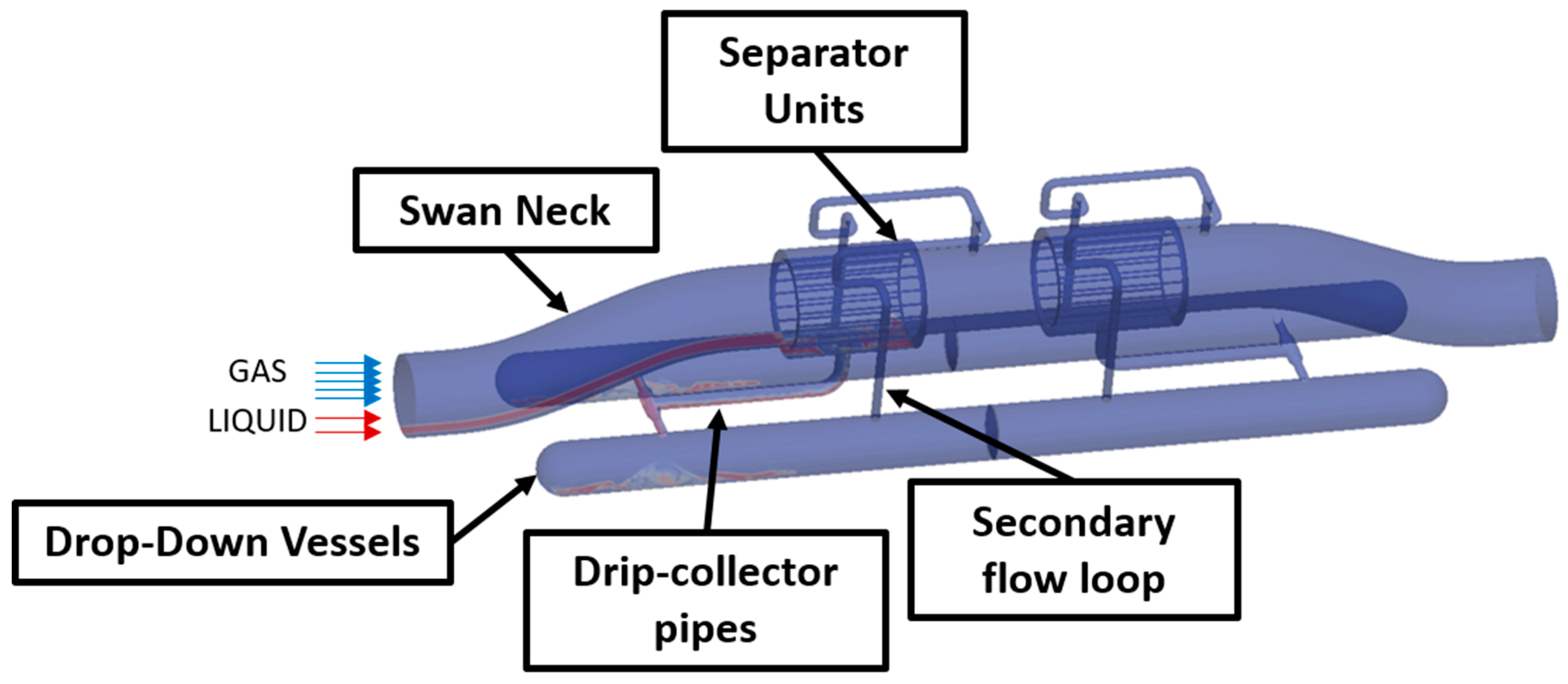
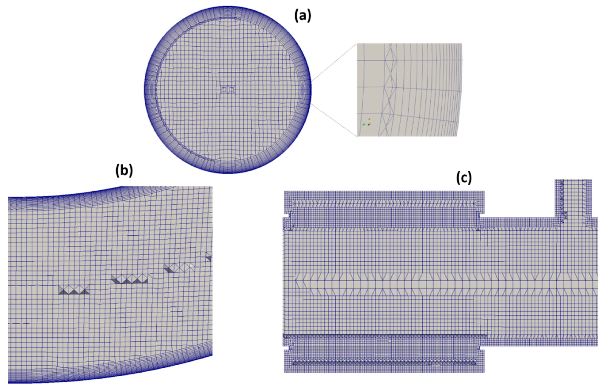
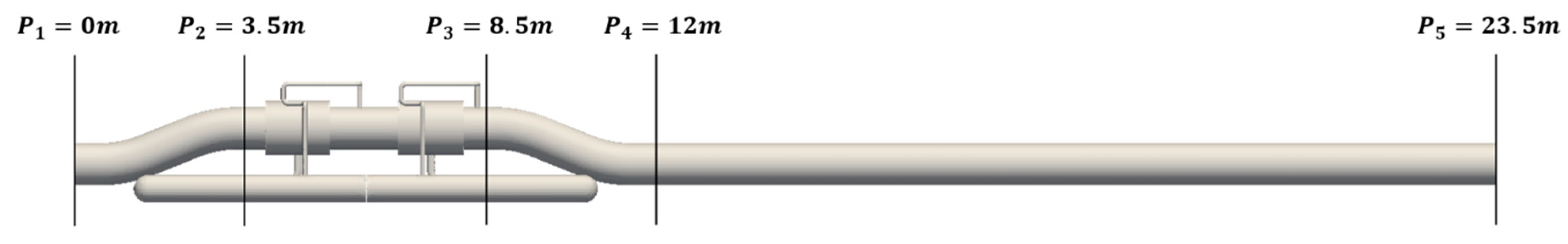
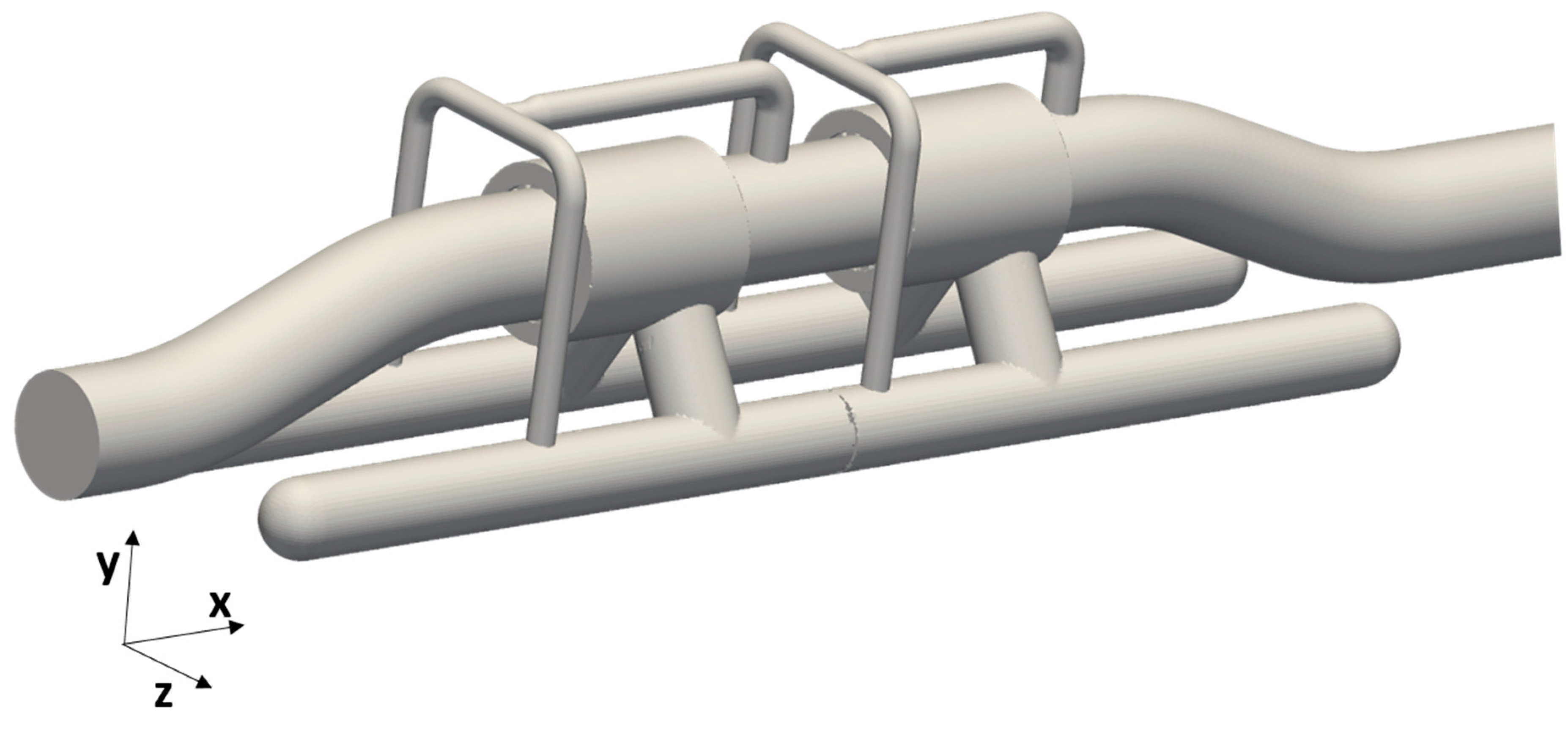
2.3. Geometry and Grid Generation

The computational meshes were generated using the open source software SnappyHexMesh (SnappyHexMesh User Guide: https://cfd.direct/openfoam/user-guide/v6-snappyHexMesh/). Initially, the geometry is meshed using a uniform hexahedral cubic cell with an average side length of $0.05\mathrm{m}$. At the swan neck, we further refined the mesh by a factor of two, i.e. cell’s side length equal to 0.025 m. We further included seventeen quadrilateral boundary layers (Figure 2a,b). The first layer has a height of $1\times {10}^{-3}\mathrm{m}$. Moving away from the boundary, the height of each subsequent layer increases by a ratio of 1.2. These boundary layers are particularly important at the inlet and swan neck, where the dynamics at the liquid–vapour interface dictate the flow behaviour.

The grid was also refined in the vicinity of the separators (Figure 2c). Specifically, we refined the initial mesh by a factor of three for all cells within a distance of 0.05 m from the separator, drip-collector pipe, and dropdown vessel walls, i.e. the cell’s side length was equal to 0.0125 m; and by a factor of two for all cells between $0.05\mathrm{m}$ and $0.35\mathrm{m}$. Finally, for the outlet pipe, the mesh was refined by a factor of two at a distance of $0.1\mathrm{m}$ from the wall.

Numerical experiments showed that the most grid-sensitive region is the inlet and swan neck, particularly close to the boundary where the fluid stratification occurs. Therefore, the grid should be sufficiently refined in the boundary layer regions. Simulations were performed on two different grids containing $2.5\times {10}^6$ and $10\times {10}^6$ cells, respectively, and it was found that the deviations of the averaged velocity values were within a range of 5% difference. Refining other regions of the geometry, e.g., separators, drop-down vessels, had minimal effect on the multiphase flow parameters investigated in this study.

In the initial geometry, the outlet was located at the bottom of the second swan neck (P4 in Figure 3). The relatively short length of the geometry is not sufficient for the flow to fully develop. Considering the subsonic nature of the flow, the zero-gradient boundary condition for the velocity at the outlet would enforce a non-developed flow condition. A possible solution would be to pose a velocity at the outlet which is not, however, known. The only other alternative is to use a longer computational domain.

Several simulations were performed in order to establish the pipe length that leads to a fully developed flow at the outlet. It was found that a pipe length of 23.5 m (approximately 25 diameters) is sufficient (P5 in Figure 3).

2.4. Validation

In the absence of experimental results, we performed validation of the present model based on the open-source CFD solver OpenFOAM [8] (Version 5, OpenFOAM Foundation, Greater London, UK, www.openfoam.org) against ANSYS CFX (Release 17.2, Canonsburg, Pensilvania, US, https://www.ansys.com/en-gb/products/fluids/ansys-cfx), a commercial CFD solver; and the Oil and Gas Simulator (OLGA) [14], a two-fluid model designed for oil-and gas applications, owned by Schlumberger.

OpenFOAM and CFX produced practically identical results, within a 3% numerical error. The present OpenFOAM model also matched the results of the software OLGA, predicting the same time and length scales associated with transient phenomena, which are discussed in Section 3.1.

Although a comparison with commercial software does not constitute an actual validation, we consider such comparisons as relevant due to the lack of experimental data in the literature. Furthermore, the comparison with the industrial code OLGA, which is used in the design of such complex systems is relevant too, in order to provide some certainy in the results

3. Results

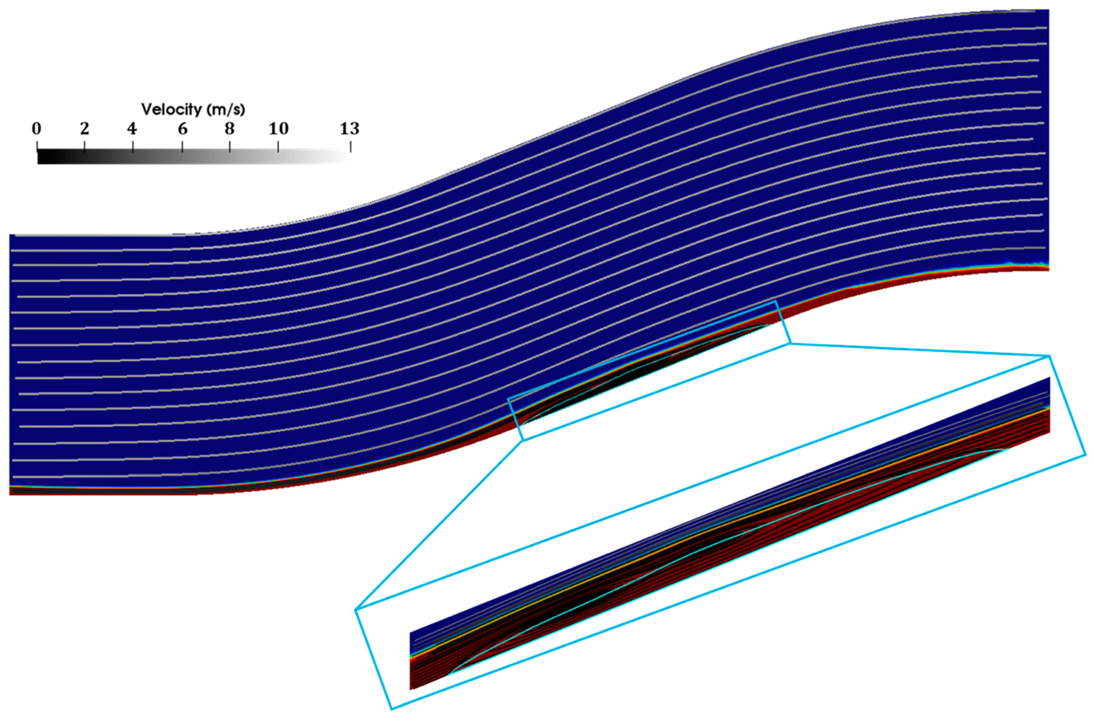
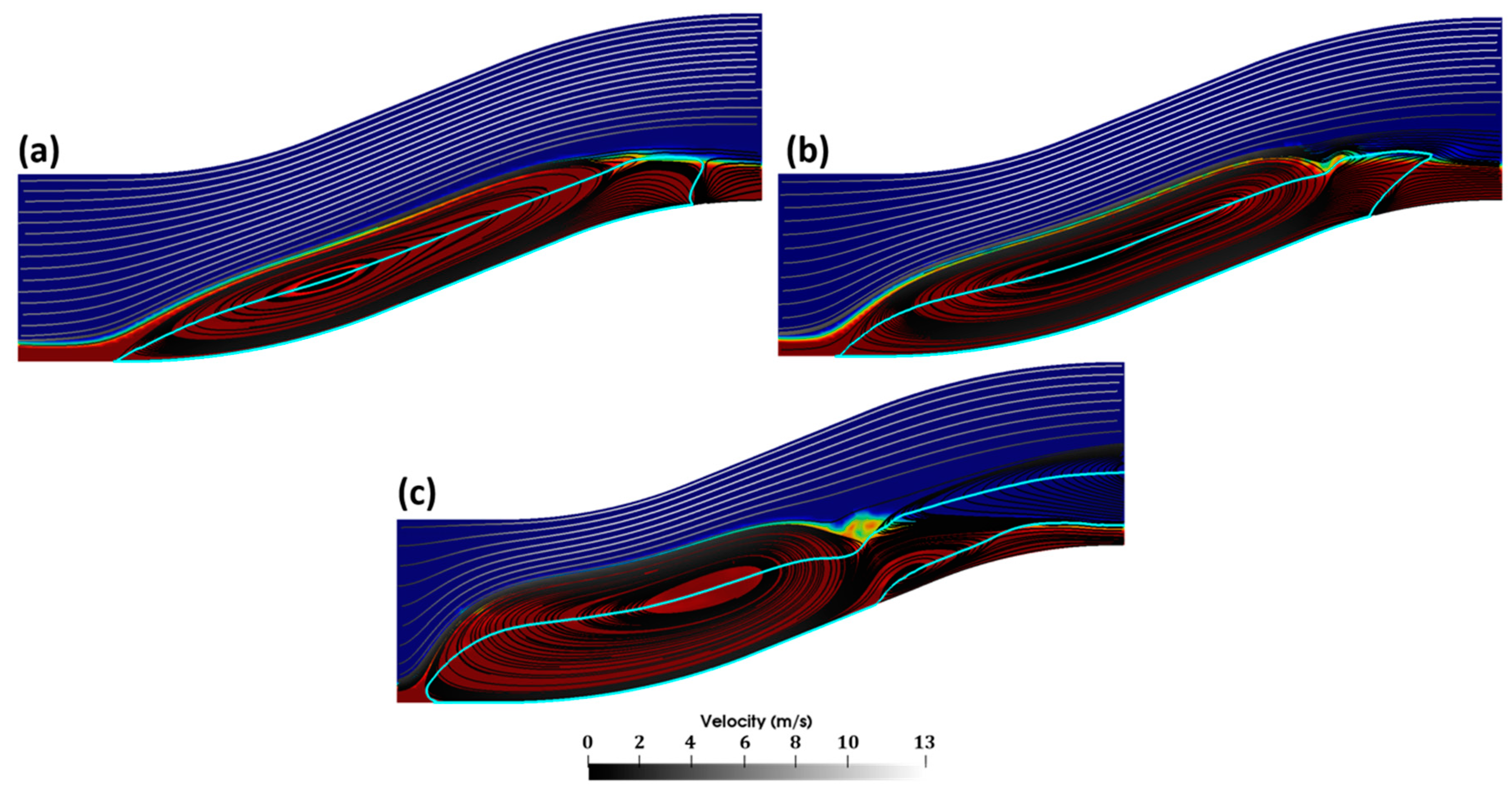
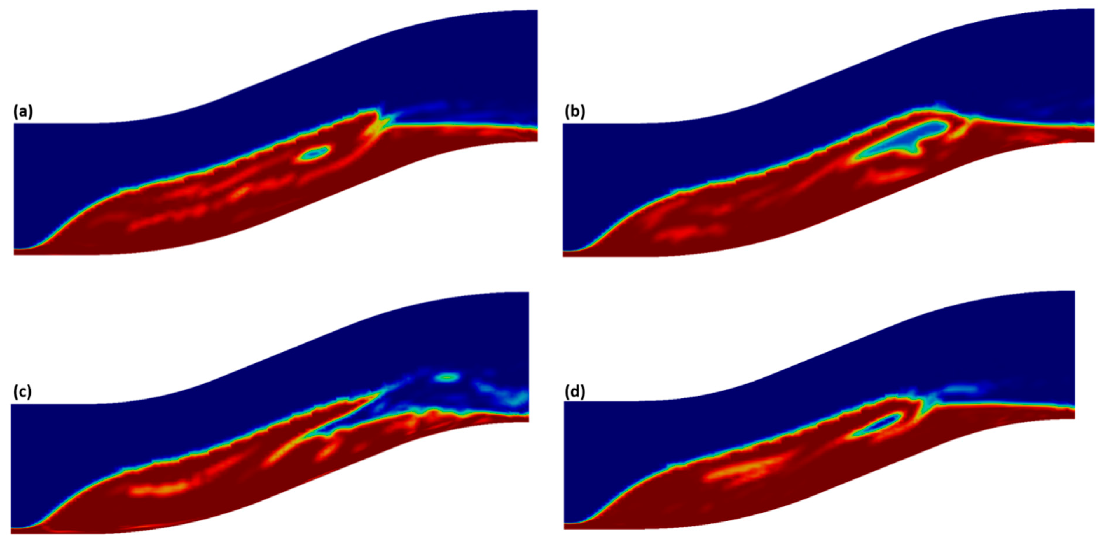
3.1. Swan Neck

The multiphase mixture initially encounters an inclined pipe, which we refer to as the swan neck. In all cases considered here, the swan neck (inclination angle, diameter etc.) remains the same.

Stratified flows across inclined surfaces result in an increase in the liquid height, thus locally restricting the gas flow. The gas velocity increases over the liquid to satisfy continuity, which in turn, causes a reduction in pressure. The lower pressure over the liquid crest causes the liquid height to further increase. This continues until gravity counters the pressure on the surface of the liquid. Analytical expressions predicting this behaviour were developed over 40 years ago [15]. These solutions, however, consider a steady state problem, with a sufficient pressure drop ensuring that the liquid has enough momentum to overcome any gravitational effects.

In highly turbulent, unsteady cases, the flow behaviour on the inclined surface is far more complex and chaotic. The liquid flow tends to separate from the inclined boundary, with the size of the separation bubble determined by the gas flow rate and, to a lesser degree, the liquid height at the inlet.

To identify the separation and reattachment points of the flow at the swan neck we first compute the component of the velocity in the direction of the flow by calculating the inner product between the velocity field and the unit vector $0.93\widehat{i}+0.37\widehat{j}$, pointing along the swan neck. We then plot the contour surface where this component is zero. These surfaces pass through the centres of the vortices, and terminate on the boundary at the separation and reattachment points (see blue lines in Figure 4 and Figure 5). There are a number of different ways to calculate the separation points in a flow [16]. Here we are considering the streamlines and the point of reverse velocity near the boundary. Streamlines provide a useful visual aid for identifying the location, size and shape of the separation bubble. We have also compared our results to other methods, such as identifying the points where the shear stress at the wall is zero or adverse pressure gradients, i.e. $dp/dx>0$, and have reached identical conclusions.

For gas velocity of approximately $7.8\mathrm{m}/\mathrm{s}$ and for a liquid height equal to $0.028\mathrm{m}$ at the inlet, the liquid flows smoothly across the swan neck and into the first separator. The liquid height increases from $0.028\mathrm{m}$ at the inlet to $0.041\mathrm{m}$ half way up the swan neck, an approximately 46% increase. The liquid crest on the inclined surface forms a small separation bubble with separation length equal to $0.1\mathrm{m}$.

For the same gas velocity but a liquid height of $0.032\mathrm{m}$ at the inlet, the height at the swan neck increases up to $0.051\mathrm{m}$, approximately 59% increase (Figure 4). The length of the separation bubble is now $0.9\mathrm{m}$, a disproportional, nine-fold increase compared to the $\approx 14\%$ increase in the liquid height between the two cases.

The majority of cases that we consider, where the gas velocity is less than $7\mathrm{m}/\mathrm{s}$, the liquid does not have enough momentum to overcome gravity and does not monotonically flow across the swan neck. The liquid separates from the boundary and starts to accumulate next to the inlet, forming a vortex that increases in size. This increase continues until the height of the liquid reaches the top of the swan neck and the liquid starts to spill into the first separator (Figure 5).

In these low gas velocity cases the size and shape of the separation bubble depends primarily on the velocity of the gas, and not on the liquid height at the inlet. The liquid flow rate only affects the speed in which the liquid reaches the top of the swan neck. Specifically, we found that as the gas velocity increases, the liquid height at the swan neck decreases, leading to a flatter vortex. As the gas velocity decreases, the liquid height at the swan significantly increases, and the separation vortex becomes almost spherical, qualitatively shown in 2D in Figure 5, and with quantitative results for the maximum liquid height along the swan neck, as well as separation and reattachment positions presented in Figure 6.

Figure 6 shows how the liquid height, as well as the separation and re-attachment points change as a function of the velocity of the gas at the inlet. The liquid height at the swan neck increases with decreasing velocity (Figure 5). Specifically, the liquid height decreases in a parabolic manner with increasing velocity (Figure 6a). Note that the data plotted in Figure 6 correspond to cases with different liquid heights at the inlet but this has a lesser effect than the effect of the gas velocity. For example, cases 3, 6, and 9 with velocities $U_g=6.4\mathrm{m}/\mathrm{s}$, $U_{g}4.79=\mathrm{m}/\mathrm{s}$, and $U_g=2.72\mathrm{m}/\mathrm{s}$, respectively, have the same liquid height at the inlet. Yet, the corresponding liquid heights at the swan neck are approximately $0.35\mathrm{m}$, $0.45\mathrm{m}$, and $0.55\mathrm{m}$, respectively.

The separation and re-attachment points are also influenced by the gas velocity (Figure 6b). For velocities less than 7 m/s, the separation point is at the bottom of the swan neck, next to the inlet. For higher velocities, i.e. greater than 7 m/s, the separation point is located near the half-way point of the swan neck. The position (x-coordinate) of the re-attachment point increases toward the top of the swan neck almost linearly with the gas velocity for $U_g<7\mathrm{m}/\mathrm{s}$. This is due to the greater pressure applied on the liquid interface, resulting in a flatter separation vortex. The re-attachment point decreases slightly for $U_g>7\mathrm{m}/\mathrm{s}$.

The shape of the separated liquid vortex has a significant impact on the flow physics downstream. The large liquid height at low gas velocities significantly restricts the cross-sectional area of the gas, compressing and accelerating it by fivefold its inlet velocity. Past the liquid crest, the gas re-expands. Depending on the curvature of the gas-liquid interface, this expansion often forms asymmetrical vortices near the top of the swan neck, reminiscent of the familiar, single-phase, sudden expansion case [17,18].

Note that Figure 5 is an instantaneous snapshot of the flow field, although the results in Figure 6 are averaged over 5 sec. Once the liquid reaches the top of the swan neck, the fluctuations of the flow separation and re-attachment points, liquid height, and liquid velocity are very small ($<5\%$). While the liquid performs small and periodic sloshing movements in the span wise direction, it doesn’t seem to affect the properties of interest. This sloshing motion does affect the motion of the asymmetrical vortices at the top of the swan neck, but again the quantities of interest remain constant with minor fluctuations. Finally, in certain cases we observed transient flow patterns, which are discussed further below. These patterns occur sparsely and do not seem to affect the performance of the separator.

The generation of vortices observed is of fundamental interest to fluid dynamics, and multiphase flows. More relevant to this study, however, this behaviour has certain consequences regarding the performance of the separator. The first is that the turbulent, vortical nature of the flow at the top of the swan neck, observed in cases with low gas velocity, disperses liquid in the gas, which can bypass both separators and lower its efficiency by up to $10\%$.

The second consequence is that traces of air gradually penetrate the liquid–gas interface (Figure 7). This forms a gas bubble that gradually increases in size. The bubble bursts once it reaches a critical diameter, and splashes liquid across the diameter of the pipe. This cycle of bubble creation and collapse was also observed using the software OLGA. For case 5, as depicted in Figure 7, OLGA predicted 21 such cycles per minute, approximating to a period of 2.85 min. In our simulations, the first cycle occurred in about 2.5 min. Furthermore, OLGA predicted a maximum bubble length of approximately 0.56 m, while our CFD model predicted a maximum length of 0.77 m. While we get discrepancies of up to 30%, note that OLGA is simulating a much larger pipeline, both before and after the separator, and the boundary conditions at the swan neck are, therefore, different.

Due to the period of time required to observe this phenomenon, we only considered it for a very small number of cases. While this needs to be further investigated, we believe that its effect on the separator efficiency is negligible for two reasons. First, most of the splashed liquid, settles down somewhere between the beginning of the first and second separators, which, therefore, does not seem to impact the overall efficiency of the separation. Second, for the cases considered here, it takes over two minutes for the bubble to grow in size and collapse. Thus, although the vortical flow affects the instantaneous efficiency of the separator, its average impact is relatively small.

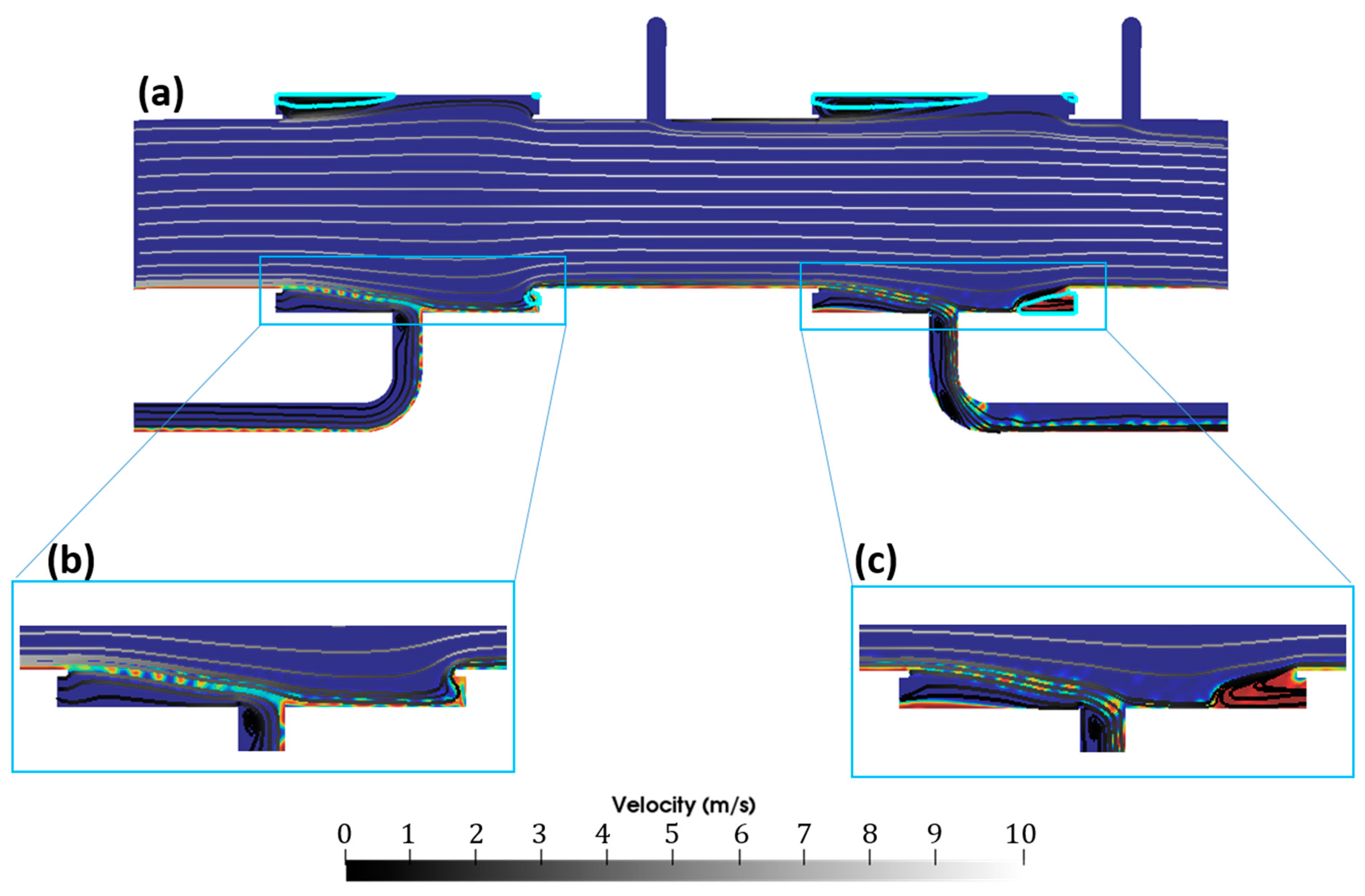
3.2. Flow in Separators

The first design considered here is shown in Figure 1 and Figure 3.

The efficiency of this design depends, almost exclusively, on the velocity of the gas. In general, the liquid at the top of the swan neck enters the first separator and hits the right wall (Figure 8a,b). A significant portion of the liquid gets sprayed over the wall and continues towards the second separator. This behaviour is qualitatively the same for all the investigated cases; the higher the gas velocity, however, the more liquid is splashed.

The liquid then enters the second separator with less momentum compared to the first separator. When the gas velocity is less than $4.5\mathrm{m}/\mathrm{s}$, the liquid settles in the bottom of the separator and starts to flow down the pipe and into the drop-down vessels. Very little liquid escapes the second separator and any reduction in efficiency is due to liquid dispersed in the air at the swan neck.

Yet, for high gas flow rates, the gas pushes the liquid against the right wall of the second separator, forming a separation bubble (Figure 8a,c). The liquid vortex leverages incoming liquid back into the main pipe, decreasing the efficiency dramatically (up to 80% reduction).

Understanding the flow behaviour and bottlenecks of the first design, the second design incorporated the following changes (Figure 9):

• The pipes leading to the dropdown vessel were moved closer to the right walls of the separators.
• The diameter of the drip-collector pipes leading to the dropdown vessel was increased significantly.
• The drip-collector pipes comprise a single straight part, diagonally connecting each separator with a drop-down vessel, rather than having one horizontal and vertical pipe, connected by an elbow.

The larger drop-collector pipes, as well as their position next to the right hand sidewall, significantly increase the efficiency of the separation. This is particularly true for cases with high gas velocities, where the first design is overall less efficient. A qualitative example can be seen by comparing case 1c between the two designs (Figure 8a cf. Figure 10). The new design clears the separators quickly, preventing the build-up of liquid on the right-hand sidewall that significantly reduced the efficiency of the separator.

The flow in the separators is shown on the $xy$ plane centred with respect to $z$ direction in Figure 11. The flow suddenly expands forming separation bubbles (see contour lines at the top part of the separators in Figure 10). The first separator unit shows practically no flow separation. The liquid flows into the drip-collector pipes, where there is practically no separation, other than an occasional small vortex on the right wall. At the bottom part of the second separator, where significantly less liquid flows in, the separation bubble is restricted to the surface just before the drip-collector pipes (Figure 10c). There is also a small vortex on the right-hand wall.

For cases with gas velocity less than $7\mathrm{m}/\mathrm{s}$, where the liquid height at the swan neck significantly increased, we observe different flow patterns at the swan neck. Specifically, a large separation bubble is formed at the bottom part of the first separator occupying up to half the height of the main pipeline. Furthermore, the greater the liquid height at the swan neck is, corresponding to the cases with the lowest gas velocity, the larger the separation bubble becomes.

This is illustrated by velocity contour lines at the separator units in Figure 12.

In general, the second design captures the stratified liquid very well. Any reduction in the efficiency of the separator is due to liquid that is dispersed in the air, which happens almost exclusively at the swan neck. In the absence of any separation bubbles, i.e., high gas velocities, the change of inclination at the top of the swan neck is enough to cause traces of liquid to become dispersed in the gas. The presence of separation bubbles at the swan neck and over the first separator seem to accentuate this entrainment of liquid, thus reducing the efficiency by up to 5%.

This observation has been further verified by designing a computational geometry identical to D2, with the only difference being that the swan neck has been replaced by a straight, horizontal geometry. We call this the manifold design. Indeed, using the same boundary conditions as before, the flow now exhibits significantly less separation in the main pipeline.

Figure 12 corresponds to identical boundary conditions as the cases in Figure 11b,c. In the absence of the swan neck, a much more regular flow pattern is observed, void of large vortices occupying a significant portion of the main pipeline. The reduced vortices in the main pipeline results in less liquid getting dispersed in the air and, subsequently, a greater efficiency. In fact, for all cases considered here, the efficiency of the manifold geometry is near ideal bulk liquid removal efficiency.

In the manifold geometries, the magnitude of the velocity is significantly reduced compared to the equivalent cases with the swan neck by approximately 50% in certain cases (Figure 12 cf. Figure 11). This is also shown in the pressure drop across the system. The pressure drop in the manifold geometries is one order of magnitude less than the pressure drop in the presence of a swan neck (Figure 13).

In the absence of the swan neck, the pressure drop generally increases with increasing gas velocity at the inlet, hence the expected outcome (Figure 13a). In the presence of the swan neck, we observe a more complex pattern. This is attributed to the increase in velocity initiated at the swan neck due to the restricted area resulting from the increased liquid height. To verify the correlation between the liquid accumulation at the inlet and the pressure drop, we plot the latter as a function of the product of the gas velocity and the square of the maximum liquid height at the swan neck (Figure 13a), where we obtain a more regular, almost linear trend.

Note that the presence or absence of a swan neck is not considered a design feature of the separator. It simply assists in the fitting of the separator in a pre-existing pipeline. Our findings suggest that including the swan neck may be accompanied by a small reduction in efficiency and a potential increase in pressure drop.

4. Conclusions

We investigated design features that may improve or reduce the efficiency of a separator. The main conclusions drawn from the CFD simulations can be summarised as follows:

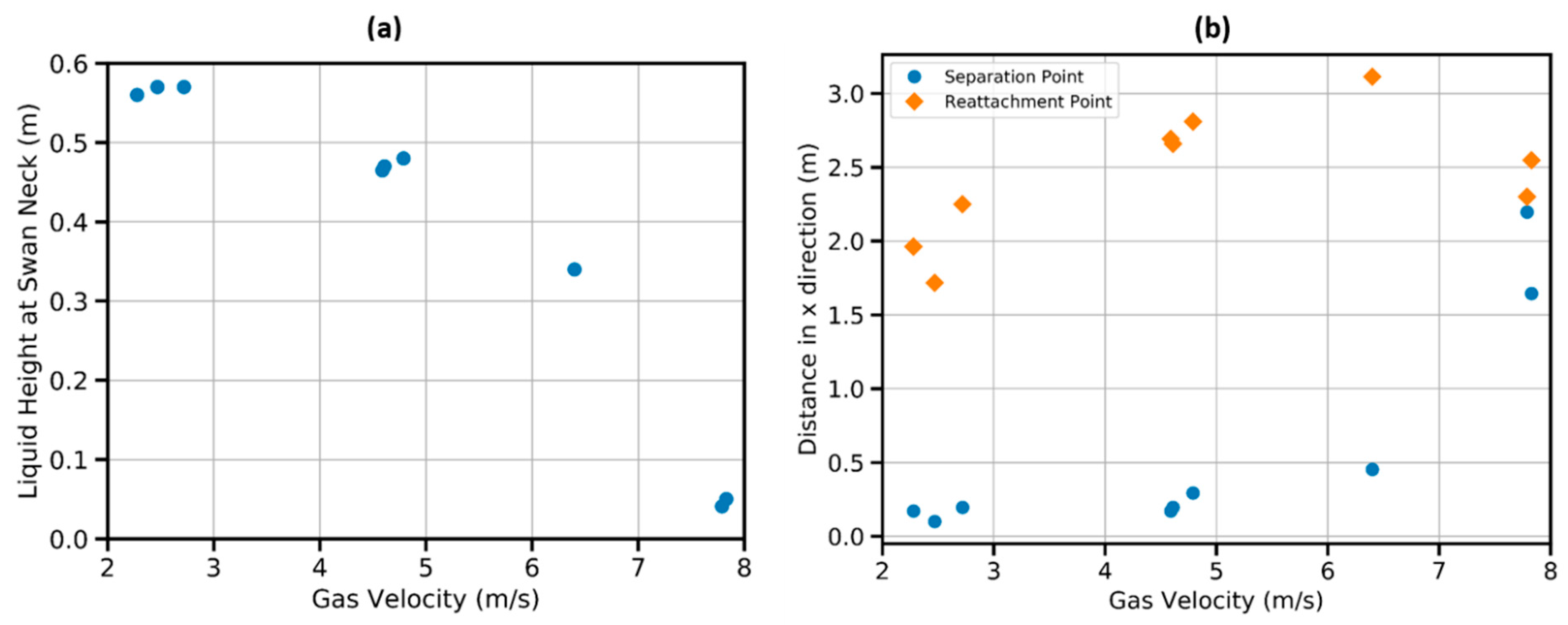
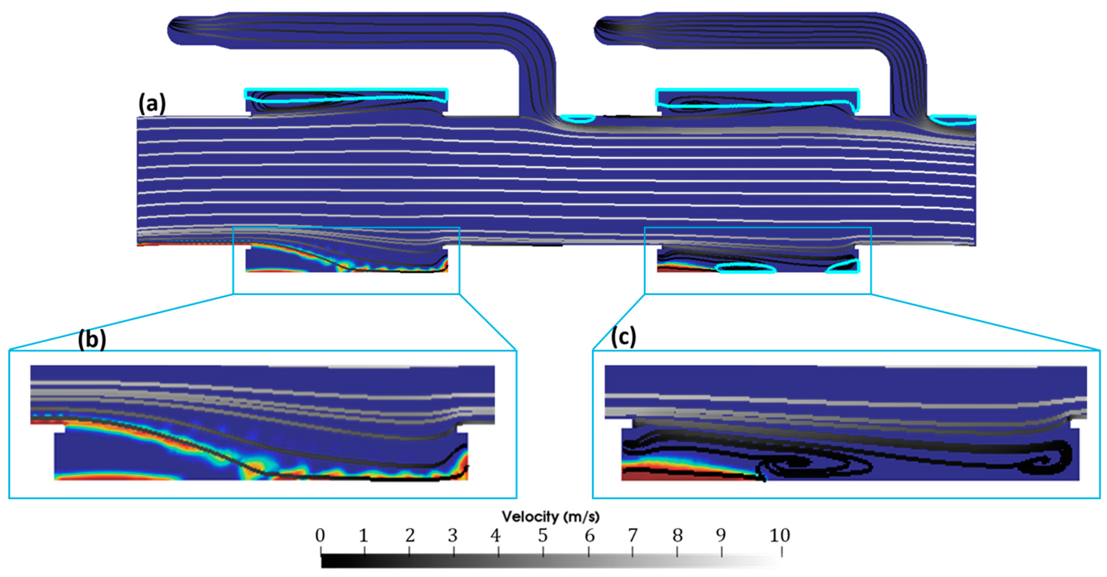
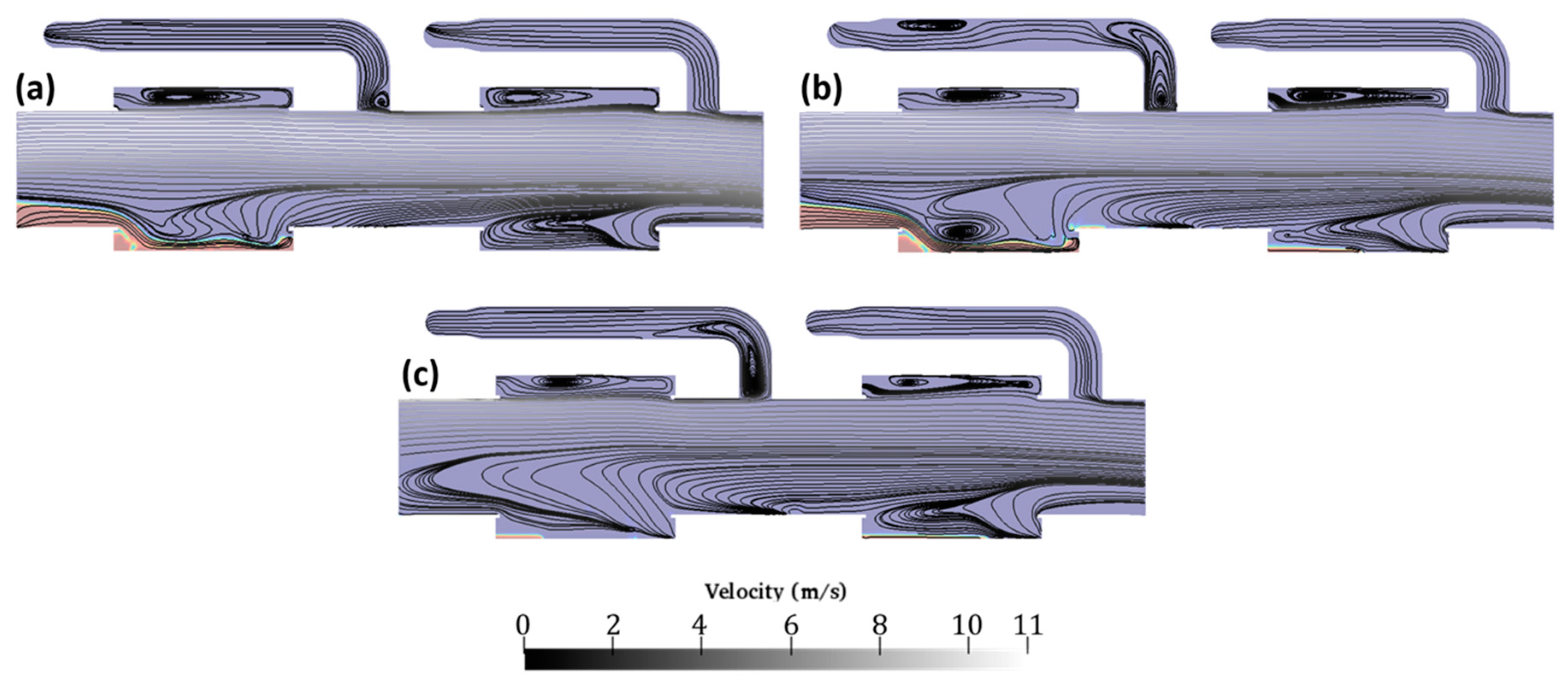
• The flow physics at the swan neck depend primarily on the gas velocity. For gas velocities greater than 7 m/s, the flow presents only a minor separation bubble at the centre of the swan neck. For lower gas velocities, the liquid detaches from the wall half way up the swan neck, and starts to accumulate next to the inlet, until the liquid reaches the top of the swan neck. Generally, for gas velocities less than 7 m/s, the separation point is at the bottom of the swan neck, next to the inlet. The position of the re-attachment point moves further up the swan neck as the velocity increases. For velocities higher than 7 m/s, both the separation and re-attachment points are close to the centre of the swan neck, at a distance approximately 1.5 m away from the inlet.
• The liquid height at the swan neck shows a parabolic decrease as a function of the gas velocity at the inlet. For the same liquid height at the inlet, changing the gas velocity from $6.4\mathrm{m}/\mathrm{s}$ to $2.72\mathrm{m}/\mathrm{s}$ resulted in a reduction of the liquid height at the swan neck, from $0.35\mathrm{m}$ to $0.55\mathrm{m}$, respectively. The gas is compressed and accelerated by the liquid crest, after which it re-expands often forming vortical structures at the top of the swan neck. These vortices tend to disperse liquid into the gas, reducing the efficiency of the separator by up to 5% compared to equivalent cases with higher gas velocities.
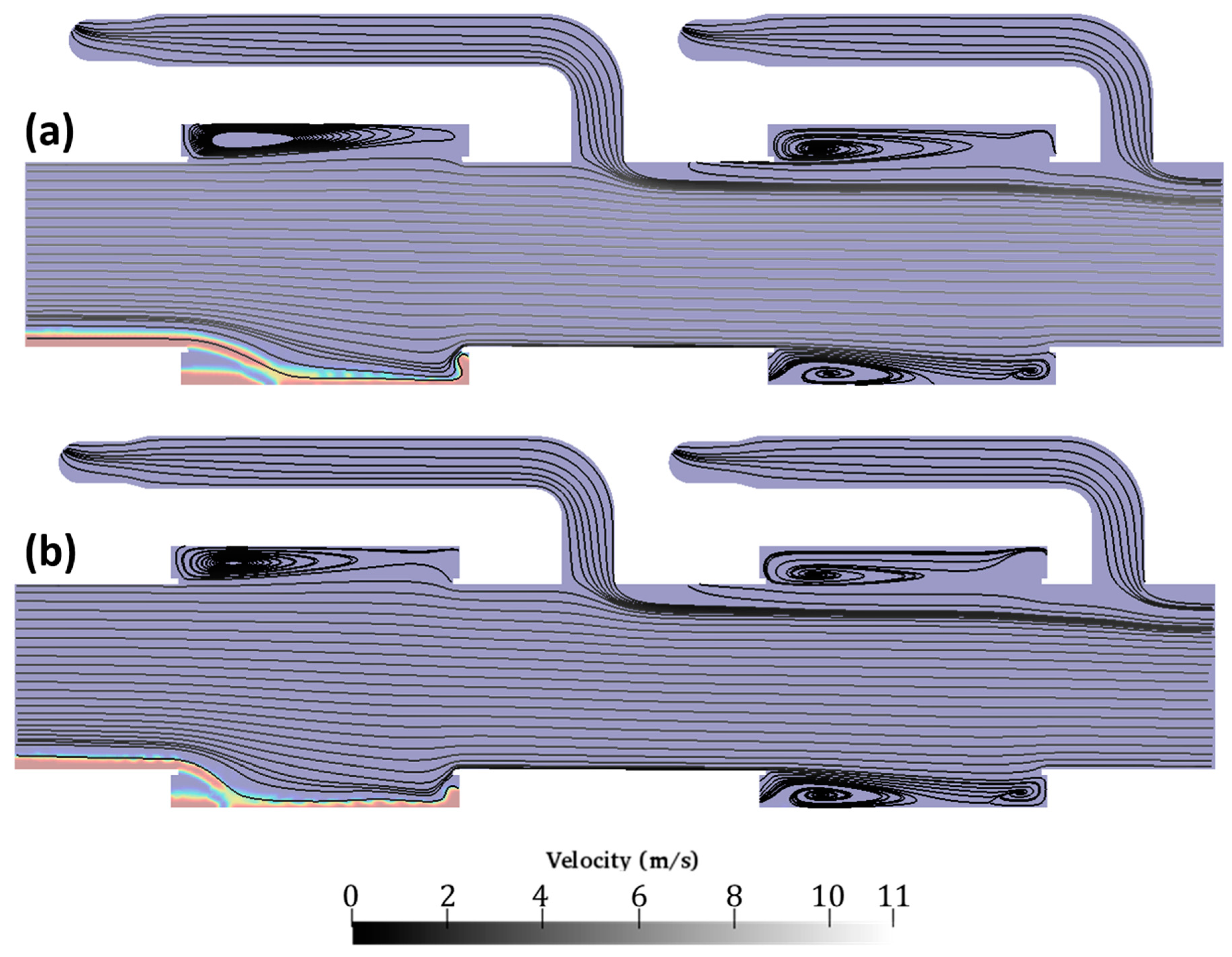
• The location of the drip-collector pipes significantly affects the efficiency of the separator at high gas velocities. Specifically, increasing the diameter of the pipes and placing them at the far right, bottom surface of each separator, as is the case for the second design considered here, significantly increases the separator’s efficiency.
• If a straight, horizontal pipe replaces the swan neck, the vertical flow patterns identified above are alleviated, and the efficiency of the separator is near ideal bulk liquid removal efficiency.
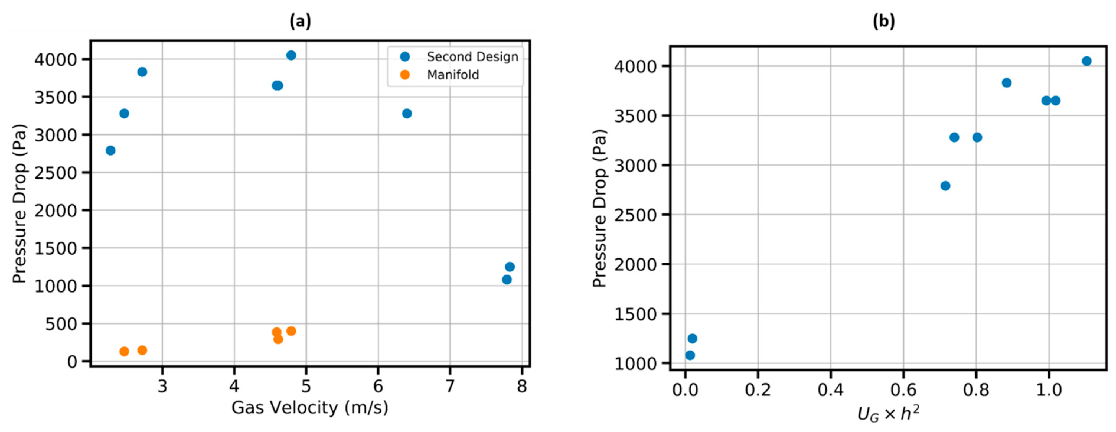
• In the absence of a swan neck, the pressure drop across the system is approximately an order of magnitude less. Furthermore, when considering a straight pipe, the pressure drop increases marginally with increasing velocity, which is the expected behaviour. By contrast, in the presence of a swan neck, the pressure drop is often higher for lower velocities. The reason for this is the aforementioned compression of the gas at the swan neck and subsequent formation of vortices near the first separator unit that restrict the flow.

In summary, we believe that the above findings are not applicable only to the designs investigated in the present study. Indeed, most flow patterns at the swan neck seem to persist regardless of the existence of the separators and are relevant to a broader set of oil and gas applications, or problems involving stratified flows through pipes.

References

- Sivalls, C.R. Oil and Gas Separation Design Manual; Sivalls Incorporated: Williston, ND, USA, 1987. [Google Scholar]
- Stewart, A.; Chamberlain, N.; Irshad, M. A new approach to gas-liquid separation. In Proceedings of the European Petroleum Conference, The Hague, The Netherlands, 20–22 October 1998. [Google Scholar]
- Powers, M.L. Analysis of gravity separation in freewater knockouts. In Proceedings of the SPE Production Engineering, New Orleans, Louisiana, 23–26 September 1990; Volume 5, pp. 52–58. [Google Scholar]
- Rosa, E.; Franca, F.; Ribeiro, G. The cyclone gas--liquid separator: Operation and mechanistic modeling. J. Pet. Sci. Eng. 2001, 32, 87–101. [Google Scholar] [CrossRef]
- Entress, J.; Pridden, D.; Baker, A. The current state of development of the VASPS subsea separation and pumping system. In Proceedings of the Offshore Technology Conference, Houston, TX, USA, 6–9 May 1991. [Google Scholar]
- Kouba, G.E.; Shoham, O.; Shirazi, S. Design and performance of gas-liquid cylindrical cyclone separators. In Proceedings of the BHR Group 7th International Meeting on Multiphase Flow, Cannes, France, 7–9 June 1995. [Google Scholar]
- Feng, J.; Chang, Y.; Peng, X.; Qu, Z. Investigation of the oil—Gas separation in a horizontal separator for oil-injected compressor units. Proc. Inst. Mech. Eng. Part A J. Power Energy 2008, 222, 403–412. [Google Scholar] [CrossRef]
- HWeller, G.; Tabor, G.; Jasak, H.; Fureby, C. A tensorial approach to computational continuum mechanics using object-oriented techniques. Comput. Phys. 1998, 12, 620–631. [Google Scholar] [CrossRef]
- Menter, F.; Esch, T. Elements of Industrial Heat Transfer Prediction. In Proceedings of the 16th Brazilian Congress of Mechanical Engineering (COBEM), Uberlandia, Minas Gerais, Brazil, 26–30 November 2001. [Google Scholar]
- Menter, F.R. Two-equation eddy-viscosity turbulence models for engineering applications. AIAA J. 1994, 32, 1598–1605. [Google Scholar] [CrossRef]
- Menter, F.R.; Kuntz, M.; Langtry, R. Ten years of industrial experience with the SST turbulence model. Turbul. Heat Mass Transf. 2003, 4, 625–632. [Google Scholar]
- Yeoh, G.H.; Tu, J. Computational Techniques for Multiphase Flows; Butterworth-Heinemann: Oxford, UK, 2019. [Google Scholar]
- Rusche, H. Computational Fluid Dynamics of Dispersed Two-Phase Flows at High Phase Fractions; Imperial College London (University of London): London, UK, 2003. [Google Scholar]
- Bendiksen, K.H.; Maines, D.; Moe, R.; Nuland, S. The dynamic two-fluid model OLGA: Theory and application. SPE Prod. Eng. 1991, 6, 171–180. [Google Scholar] [CrossRef]
- Taitel, Y.; Dukler, A. A model for predicting flow regime transitions in horizontal and near horizontal gas-liquid flow. AIChE J. 1976, 22, 47–55. [Google Scholar] [CrossRef]
- Cebeci, T.; Mosinskis, G.; Smith, A.O. Calculation of separation points in incompressible turbulent flows. J. Aircr. 1972, 9, 618–624. [Google Scholar] [CrossRef]
- Drikakis, D. Bifurcation phenomena in incompressible sudden expansion flows. Phys. Fluids 1997, 9, 76–87. [Google Scholar] [CrossRef]
- Neofytou, P.; Drikakis, D. Non-Newtonian flow instability in a channel with a sudden expansion. J. Non-Newton. Fluid Mech. 2003, 111, 127–150. [Google Scholar] [CrossRef]