1. Introduction
Renewables presently supply more than 20% of the world’s energy demand and represented almost two-thirds of the new net electricity capacity additions in 2016 [
1]. The majority of the growth in renewables comes from solar power and photovoltaics grew faster than any other energy resource in 2016 [
1]. To meet future energy demands and accelerate decarbonisation in all sectors in order to be on track to meet long-term climate goals, a diversified set of energy sources is needed. A significant part of global renewable energy resources is stored in oceans. Wave energy has attracted the attention of the scientific community and the energy industry especially since the 1970s, in connection to the oil crisis of 1973 [
2], but the first patent for a device to convert wave energy into usable energy was filed in France as early as 1799 [
2,
3].
There are several potential advantages of utilizing wave energy for renewable electric power generation [
4]. Through the years, technological breakthroughs in relevant disciplines have enabled wave energy device development to accelerate and testing has shown promising results [
5]. However, costs to implement modern wave energy converters (WECs) are currently higher than those of other renewable energy technologies [
6] and combined with the unproven status of the technologies this has hindered investors’ confidence in the sector. With a small absolute contribution, ocean power is expected to scale up from small- to medium-size demonstration projects over the coming years. The International Energy Agency [
7] reports that detailed cost analysis for wave energy conducted for the US Department of Energy concluded that costs could decrease significantly as technology moves towards more commercial scale.
Before an implementation of WECs, a thorough assessment of the conditions should be conducted for the area of interest. A first step would be a spatio-temporal energy resource assessment and availability analysis. The wave power resource, or wave energy potential, has been assessed in many recent studies, e.g., for coastal ocean areas [
8,
9], for seas [
10,
11] and for lake Erie [
12]. Additional references on wave energy resource assessments are also found listed by country or region in Chen et al. [
13] and an overview of the global distribution of wave power resources is discussed in Kasiulis et al. [
14].
The Baltic Sea is a relatively large semi-enclosed sea bounded by nine countries with an estimated combined area of about 435,000
. Overall, maps for the theoretical wave energy potential, or wave power, for such a large study area provide an excellent overall view of available wave resources for energy conversion. For the Baltic Sea region, several previous studies have also been conducted, some of which have neglected the influence from seasonal ice conditions [
11,
15] or have focused their studies on areas which are almost always ice-free [
16,
17,
18]. The seasonal ice-cover is, however, known to influence the wave climate and Tuomi et al. [
19] suggested ways to calculate different types of statistics taking the ice-time into account.
The Baltic Sea and the Swedish west coast are of high interest as the government of Sweden, together with a broad coalition of political parties, has set a target to have 100% renewable electricity production by 2040 [
20]. It is clear from works such as [
21,
22,
23,
24] that a high horizontal resolution for the wave model is required to effectively capture the spatial variations of waves near coasts. Wave energy conversion sites generally benefit from being located closer rather than further away from suitable harbors in order to facilitate and reduce the costs of transportation to and from the site. Being close to the shore also reduces the cost of power transmission. Coarse numerical wave model results are therefore of limited use in assessing the near-shore wave energy resource. Existing wave energy converter test sites have so far been placed within 17 km from the shore in water depths less than 100 m (see Figure 14 in [
6]), requiring fine detailed bathymetry data to make a joint analysis and identification of potentially interesting pilot sites for WECs. Future large-scale commercial wave energy park installations may very well be located further from the shore as well as in deeper waters, depending on several conditions at accessible and available sites, WEC and transmission technology, the possibility of using ROV (remotely operated underwater vehicle) robotics in sea operation and maintenance, among many other aspects including economy of scale and the price of electricity.
In a multi-disciplinary project, a high horizontal resolution of the wave field information can be useful as it can be combined with high-resolution topographic data, geotechnical information, environmental classifications and other types of information [
22] relevant in site selection. The size of the proposed wave energy park installations may often range from around 250 by 250 m to 1
in size and here we report results from a high-resolution 16-year wave hindcast (at about 1
) with the aim to provide estimates of the theoretical wave energy potential for the Baltic Sea and along the Swedish west coast. Previous studies for the region include Weisse et al. [
25] with 5 times lower resolution, and Reistad et al. [
26] with about 10 times lower resolution. Björkqvist et al. [
24] is one of the most detailed studies of wave climate, over a long time period of 41 years, conducted for this region using a wave hindcast dataset that included modeled sea ice at about 1 nmi horizontal resolution (about 2 km), but no wave energy resource assessment was conducted. An extremely detailed 100 m horizontal resolution simulation, but for a much more limited domain, has been performed for the Lithuanian coast [
27]. The dataset produced here also provides necessary statistical information for detailed calculations of technical wave energy potential in upcoming studies as this study is only one part of a larger project on marine energy conversion in the SEEZ [
22]. The total wave energy resource of Sweden has no precise estimate [
22,
28] and further study is needed.
One of our aims is to introduce a partly new and innovative way to present the wave power resource using the distance from resolved land as a factor that is highly influential on the wave field, through its connection to processes that reduce wave energy near the coast. These include the fetch conditions, breaking wave effects (shoaling and refraction), bottom friction as well as shadowing effects from islands. The distance from the coast parameter provides the basis for a relative resource classification method introduced in this work. While new for the Baltic Sea, a similar method has been used in Nobre et al. [
29] for some parts of the Portuguese coast. The results are illustrated and focused on the Swedish exclusive economic zone, but the classification could be carried out in a similar way for other basins around the world, or using national marine boundaries to facilitate assessment of the most promising wave energy resource areas in different countries. Another aim of this paper is to use high-resolution wave modeling to investigate the Baltic Sea area for its wave power resource. The results will be discussed both on a basin level and at a wave energy converter park level which is unique for the studied area. A detailed assessment is also carried out to characterize the directional dependence on the wave power resource and its effect on the temporal availability of the wave energy. This could be of great importance for fetch-limited seas at high latitudes as there is great seasonal and directional variability in the wave field parameters.
This paper is structured as follows: In
Section 2, the numerical wave modeling and datasets are introduced. This is followed in
Section 3 by an evaluation of the wave model results using wave buoy data. Then, results that characterize the wave power resource for Swedish conditions are presented and discussed in
Section 4. Wave power estimates for the SEEZ are also compared and contrasted with results for the Baltic Sea and a relative resource classification and simple joint analysis is carried out on some other aspects such as water depth in
Section 5. A brief outlook for more aspects to be studied for this region is given and results are discussed in
Section 3,
Section 4 and
Section 5. Finally, a summary and conclusions on the main results are found in
Section 6.
3. Model Evaluation
Overall, the measured and hindcast mean significant wave heights in
Table 1 agree regarding the range of encountered values for the region. Measured values are between 0.37 m (close to coast at Oskarsgrundet) and 1.24 m (at Södra Östersjön wave buoy representing more open sea conditions). The corresponding modeled values calculated for the full 16 years of simulation were found to be 0.34 m and 1.21 m.
Table 1 also shows estimates of the 95th percentile for significant wave height, which indicates that, in general, slightly higher values are estimated from the hindcast compared to the measurements. Nevertheless, the range of variations in the measurements—from 0.78 m at Oskarsgrundet to 3.04 m at Södra Östersjön—is well estimated by the hindcast values, which fall between 0.87 and 3.11 m. The differences observed in
Table 1 can partly be explained by differences in time periods between measurements and model values, but a slight overestimation of the variability in the significant wave height will later be shown when the coinciding data are evaluated.
The distributions of the measured values of significant wave height in
Figure 1 (a) and hindcast values in (b) also show a good agreement for many sites, but with some larger differences most obviously seen for Oskarsgrundet and Trubaduren locations (red full or dotted lines marked with squares). In this figure, only data from wave records with more than 15,000 half-hours are used to form the measured distributions. Only data up to 4.5 m are shown since larger significant wave heights are rare. Wave heights above 8 m occur in some basins [
43], but extreme conditions for the Baltic Sea are not in focus here.
On the west coast of Sweden, some issues with either too short fetch conditions from the North Sea used in the modeling or missing wave–current interactions caused some underestimation of significant wave heights and wave periods when the evaluation of coinciding data was performed. Further testing with a wave–atmosphere–ocean-coupled model system for a short time period has indicated that wave–current interaction could be important (personal communication with Lichuan Wu at Uppsala University) and inclusion of boundary conditions from a North Sea wave model may have alleviated the issue.
A statistical post-processing correction was applied for the Swedish west coast based on a monthly wave index method, which is essentially identical to a geostrophic wind index method used in wind energy applications described further in Nilsson and Bergström [
44]. Here, it was, however, applied to correct wave information (significant wave height and energy period) using a modeled wave dataset from Weisse et al. [
25], which has taken into account the potentially long fetch conditions for the region by application of nested simulations covering the North Atlantic ocean, but performed the simulations at about 5 km horizontal resolution. All coinciding times with ice-free conditions in both datasets were used to form the monthly correction factors.
For the wave buoy Väderöarna WR which has the largest amount of coinciding measured and modeled data, the bias was reduced from −0.25 m down to −0.09 m. At the buoy Läsö Ost, the bias was also reduced from −0.16 m to −0.12 m, but at the wave buoy Trubaduren located closer to coast a small overestimation of significant wave height of 0.01 m was increased to 0.06 m after the correction was applied. The overall error statistics considering all available wave records from the Swedish west coast showed improvements by the procedure. The wave power resource estimate for the two datasets differed at most by about 10% when all coinciding data were used.
It is worth noting that the correction approach only used the two modeled datasets. No calibration using the measurements was applied, which could in future work be possible to use for further improved wave energy resource estimations for specific sites with available wave data. Such an assessment has, however, already been performed for the west coast of Sweden in the study by Waters et al. [
45] with overall similar results to those presented here. Since the wave buoy measurements were not used for calibration, they can be used to evaluate the performance of the produced wave hindcast dataset, which is our aim here.
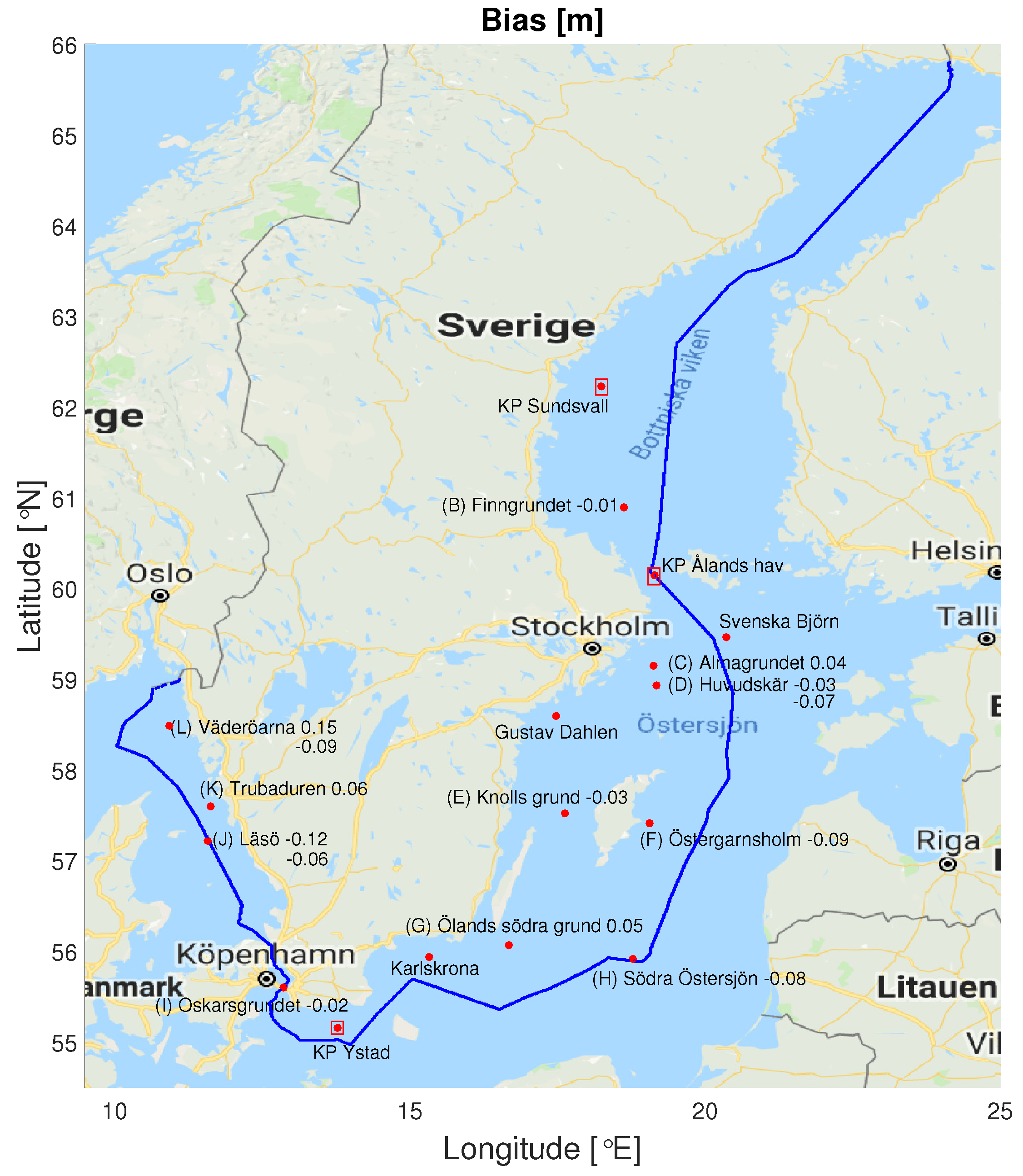
Table 2 lists the bias for all wave records that has coinciding measured and modeled data. This bias is also shown in
Figure 2 next to the location name on a geographical map. There are 14 sites with measurements, of which three have two wave records for the same location in the SMHI database, making it, in total, 17 wave records used for the evaluation. Apart from the 14 wave measurement locations, three additional sites in
Figure 2 are marked with red dots inside squares on the map and also marked with the names: KP Sundsvall, KP Ålands hav and KP Ystad. Seventeen selected grid point locations are marked in total where full two-dimensional directional wave spectra and additional wave statistics were saved on an hourly basis for testing and validation purposes. Wave buoy data from SMHI are available at
http://opendata-download-ocobs.smhi.se/explore/ and for the wave buoy outside Östergarnsholm run by the Finnish Meteorological Institute (FMI) by contacting the author group. The bias varies between −0.12 m and 0.15 m for different wave records, with an overall bias of −0.06 m. No obvious systematic difference between geographical regions is present, which confirms that the dataset is suitable for a relative comparison between sub-basins within the SEEZ.
In
Table 2, the centered root-mean-square error (CRMSE), linear correlation coefficient and standard deviation of the measurements are also listed. High correlations above 0.90 are shown in comparison to all wave records except at Oskarsgrundet which has 0.71. Oskarsgrundet is located closest to the coast and has the lowest observed standard deviation of all sites with 0.20 m, because of its relatively low wave climate. The root-mean square errors range from 0.17 m to 0.38 m with an overall average of 0.26 m, which is similar to reported error statistics of previous wave modeling efforts [
19,
21,
24].
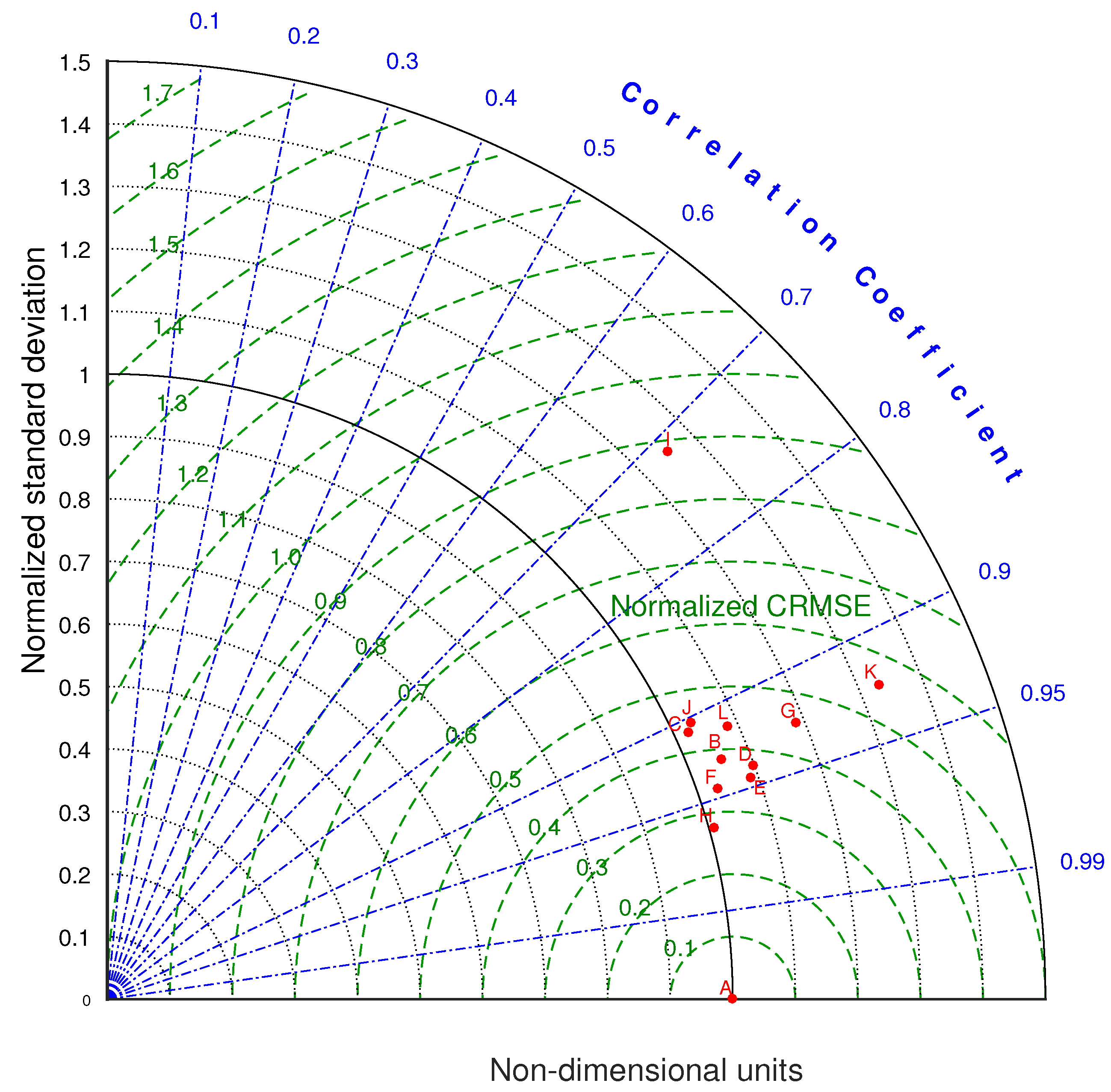
A good way to investigate model behavior and compare modeling errors at different sites is to scale the standard deviation of significant wave height from the model as well as the CRMSE with the measured standard deviation and display the result in a Taylor diagram [
46], as shown in
Figure 3. The evaluation metrics used are properly defined in
Appendix A. The Taylor diagram uses the law of cosines to display how the normalized wave hindcast statistics (CRMSE/
,
and the linear correlation coefficient
) compare at different sites and relative to the observed values.
Figure 3 reveals that all sites except site K (Trubaduren) and I (Oskarsgrundet) have a normalized CRMSE of less than 0.45 since each green dashed line away from the observed point A indicates a
times CRMSE/
increase. Site G (Ölands södra grund) has a standard deviation of about 19% larger than observed, which may be related to special topographic conditions in this area. Apart from the three above mentioned sites, the other locations all show standard deviations between 0% and 10% higher than the observed values. This is shown by their placement between the black line—indicating a ratio 1 for the standard deviations—and the first dashed black line on the right, indicating a ratio of 1.1. This can be considered as a good behavior for the hindcast dataset since the buoy locations are geographically spread out and a relative assessment for the SEEZ is one of our objectives.
The linear correlation coefficient is, as previously discussed, above 0.90 for all sites except Oskarsgrundet (I), which is close to coasts and islands from several directions. Trubaduren is also located relatively close to coast (8.4 km) and in a geographical location which is complex. There are some islands nearby and there is proximity to several coastlines, which may further increase the difficulty to obtain more accurate wave model results. At the Östergarnsholm site (F) in the Baltic Sea, the distance of 8.5 km to the island of Gotland is similar, and there is a smaller island named Östergarnsholm about 4 km from the buoy location. This island was too small to be resolved on the model grid, but otherwise the archipelago is less complicated on the east side of Gotland; overall, the wave model showed good error statistics at Östergarnsholm, with an overestimation of only about 3% for
, a linear correlation of 0.95 and a CRMSE of 0.21 m. Nevertheless, it is likely that relative errors may be somewhat larger for locations closer to the coast, especially in certain regions within the SEEZ that has a complex archipelago. This is also consistent with conclusions from more focused wave modeling efforts in archipelagos and near-shore regions [
23,
36].
4. Wave Power Resources
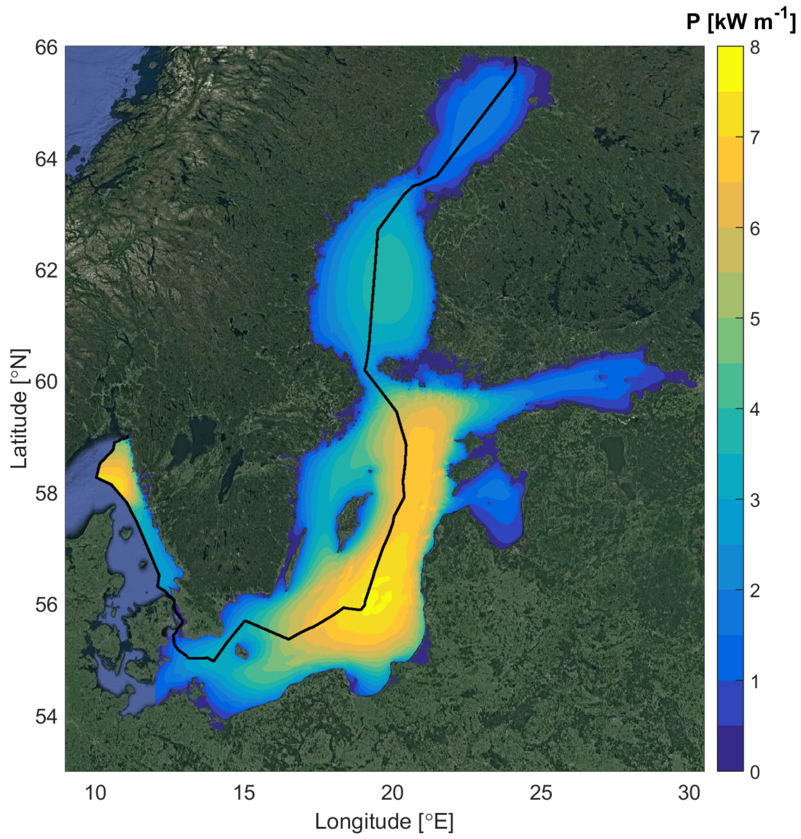
In
Figure 4, the annually averaged wave power P is shown, calculated using the relationship:
where
is the significant wave height,
is the density of seawater,
g is the acceleration of gravity,
is the energy period and
is the group velocity determined from the energy period and the water depth,
h. See
Appendix B for further details, references and a brief discussion on the results from a method comparison at two sites.
Wave power estimates for the Baltic Sea and SEEZ are based on the 16-year hourly wave hindcast values. Ice-time-included statistics are displayed, where the wave power P is set to zero when the ice concentration seen by the model is larger than 30%. Tuomi et al. [
19] suggested similar ice-time-included statistics for mean significant wave height in basins with seasonal ice cover. The wave resource is about 8 kW/m in the outer parts of the SEEZ in the middle of the Baltic Sea and varies down to nearly no wave energy in sheltered areas close to land. On the west coast of Sweden, there is also a higher amount of wave energy closer to the coast in the northern part of the SEEZ, which is less sheltered by Denmark. Comparable wave power estimates can be seen along the western coastal areas in the Baltic Proper. This is related to the predominant wind directions from west and southwest which result in higher wave energy near the western shores than near the eastern shores (e.g., [
19,
24,
27]). Similar results have previously been found also for the average annual wave energy density [
17].
4.1. Wave Energy in Different Basins
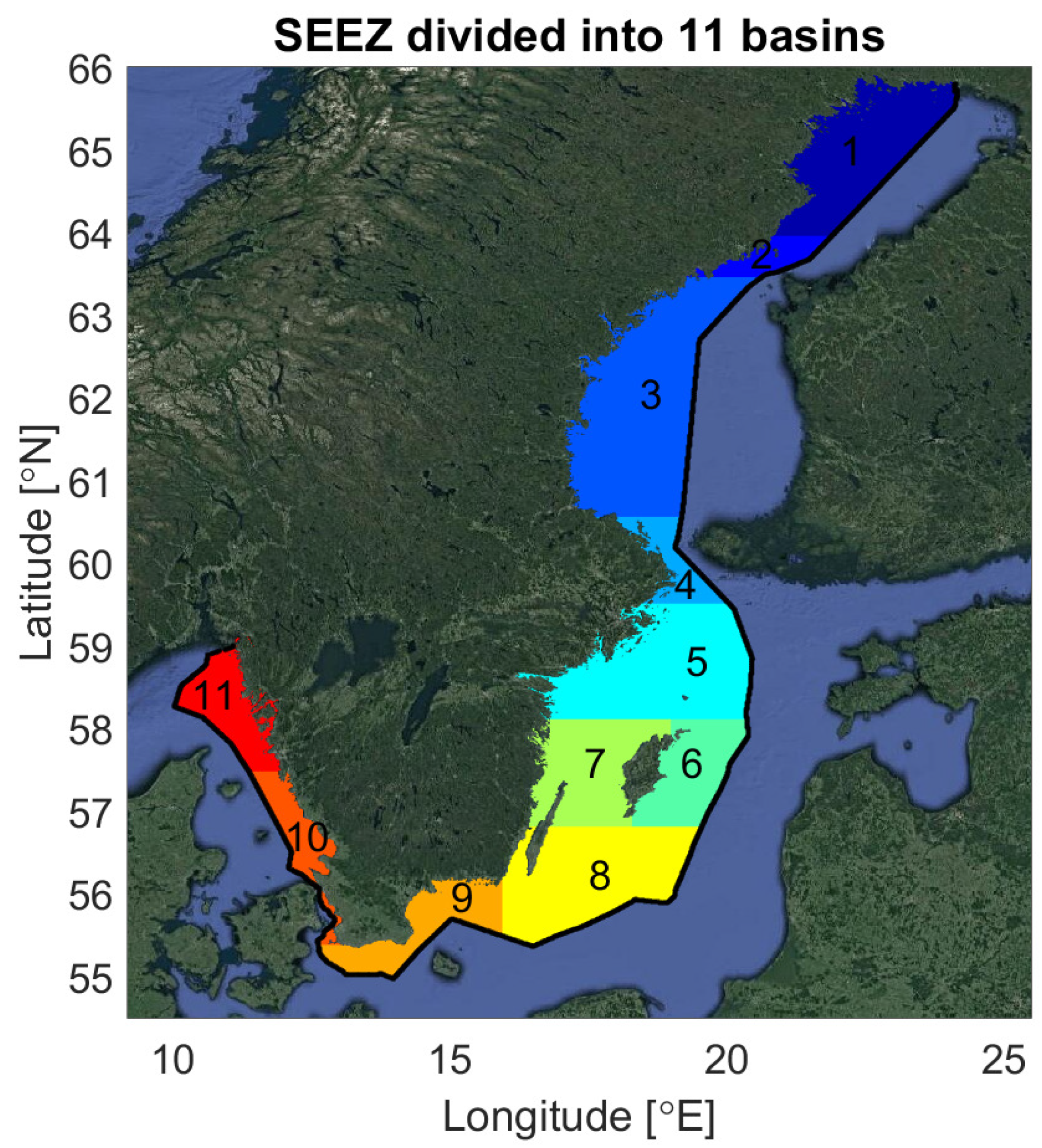
For a further discussion on the wave power resource variations within the SEEZ, the SEEZ region is split into 11 smaller basins, as shown in
Figure 5. The basins are named 1 to 11, starting from the most northern latitudes and continuing first within the Baltic Sea, and finally including two basins on the Swedish west coast. The dominant wave directions, water depth and wave power resource were considered when choosing the locations of the basins.
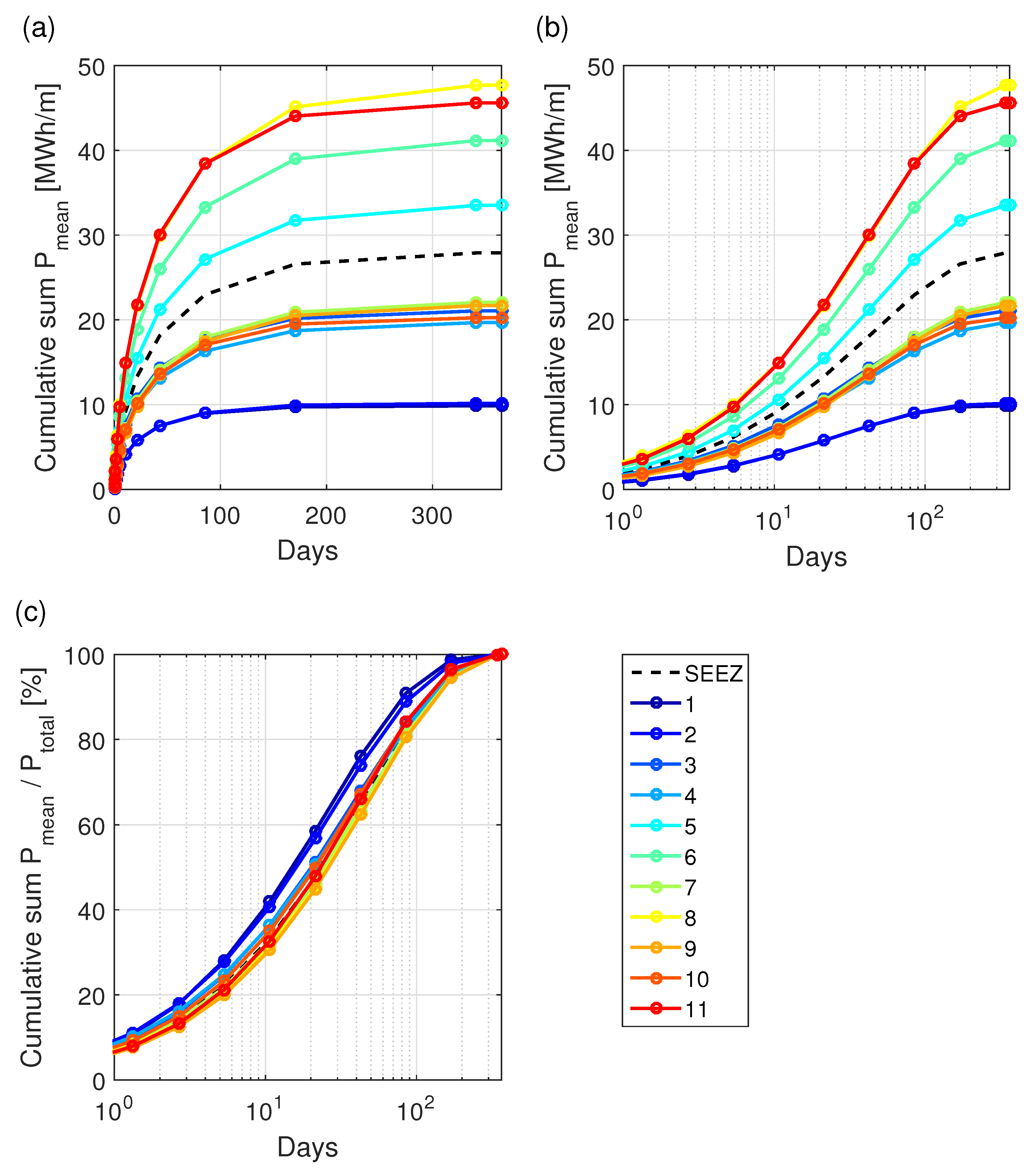
For a brief comparative overview of the mean behavior of the wave energy resource in different basins, a cumulative sum of P arranged from its highest to its lowest value is shown in
Figure 6a with different colored lines corresponding to different basins. It can be seen that the summation to the annual mean wave energy resource in basin 8 and 11 is the highest and reaches 48 and 45 MWh/m/year, respectively. This is followed by basins 6 and 5 which have 41 and 34 MWh/m/year as an annually averaged theoretical wave energy potential. The two most northern basins 1 and 2 show the lowest wave energy potentials, on average 10 MWh/m/year, and all other basins group together with 19 to 22 MWh/m/year. The mean for all of the SEEZ is 28 MWh/m/year.
In
Figure 6b, the same data are shown with a logarithmic
x-axis to more easily identify how much of the wave energy comes from relatively short periods of time each year. The strongest storms each year for this region will, due to the synoptic weather conditions, bring with them a surge in wave energy that lasts only a few hours to a day or so. This is due to the relatively short fetch conditions, which result in the predominance of wind sea over swell systems. The summation of ordered wave power values P reveals this aspect of the wave hindcast data. For instance, it can be seen in (b) for basin 8 and 11 that 15 MWh/m is condensed to occur during a time period that amounts, in total, to only about 10 days per year.
To investigate and compare this behavior for different basins, it becomes natural to scale also the
y-axis by normalizing with the annual average (
Figure 6c). The two most northern basins have about 40% of their wave energy resource summed up in about 10 days, while the comparable percentage for basins 8 and 9 is closer to 30%. This behavior is more prominent for the most northern basins because of their more extensive ice-cover. Each year, the longer ice-time will cause low or no wave energy potential for several months that would otherwise frequently have high wind waves brought on by intense passing low pressure systems.
4.2. The Ice Cover
To investigate the effect of the ice-cover on the wave power potential, the difference between our ice-time-included wave power estimate and a so-called ice-free statistic from Tuomi et al. [
19] was calculated, where averaging of P was done only for all the times when the model did not see ice. In this case, this corresponds to ice concentrations less than 30%.
Figure 7 clearly shows that in the northern part of the Baltic Sea the wave power may have been reduced by up to 900 W/m, which can constitute even up to 50% of the wave power resource in some regions. Some minor effects on the wave resource between 0 and 150 W/m from the ice-cover can also be seen south of latitude 59 locally around some coastal areas, but most significantly it is basins 1 and 2 that are affected followed by basins 3, 4 and parts of basin 5.
Similar results discussing the influence of ice on the mean significant wave height as well as percentiles of significant wave heights were presented in Björkqvist et al. [
24]. In [
24], a clear effect in the Gulf of Riga was not seen but a couple of reasons differ between these studies. Here, interpolated ice-concentrations from observations were used; Björkqvist et al. [
24] used an ice-model coupled to the wave modeling. The different studies also have different time periods. Björkqvist et al. [
24] let the wave model see the ice at 50% ice concentration, whereas in the present work the ice is considered at 30% similar to the setup used in Tuomi et al. [
19].
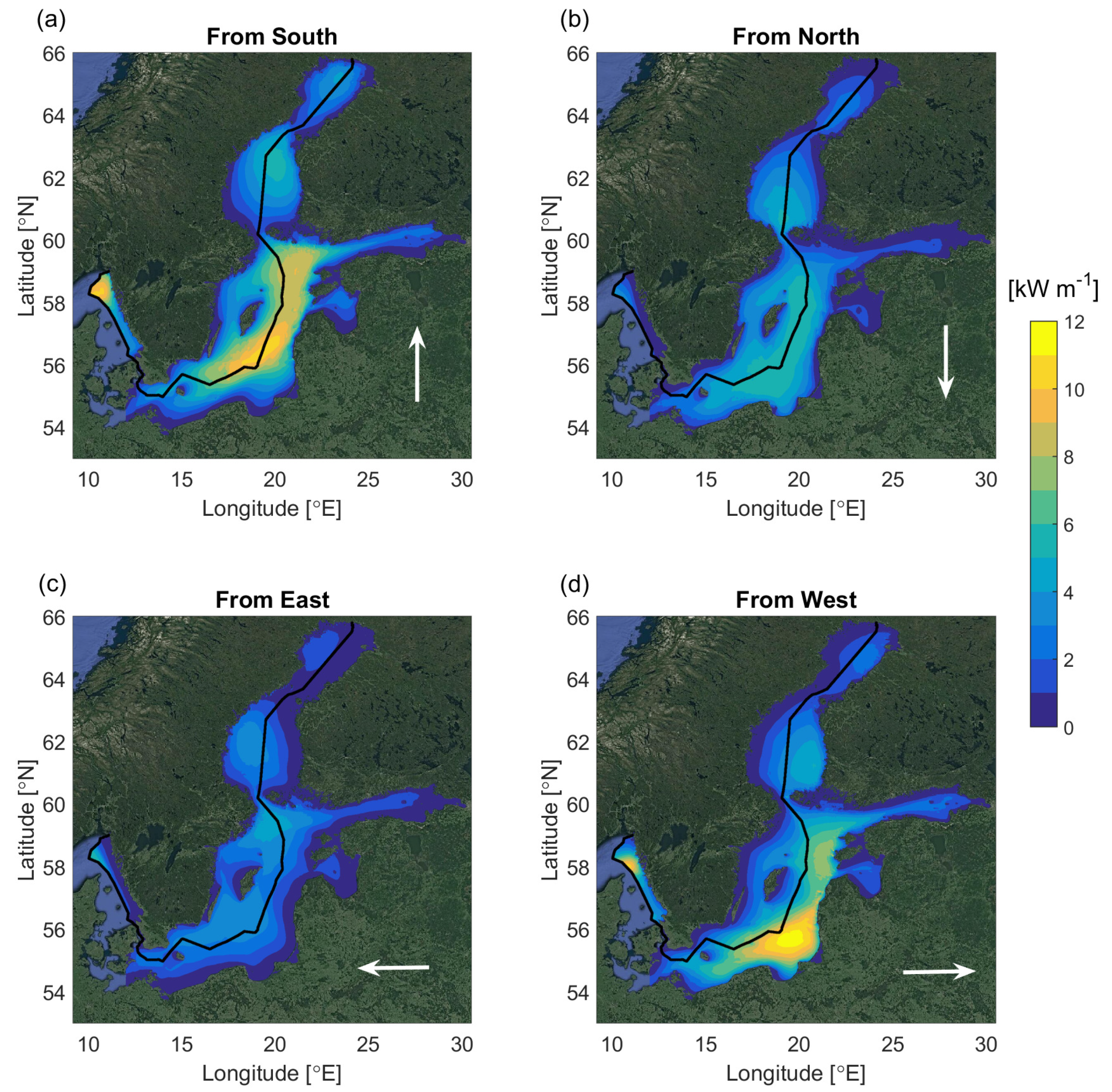
4.3. Directional Dependence
Different directions correspond to different fetch conditions and can therefore behave variably in terms of the available average wave power. Conditionally averaged wave power estimates for separate directional sectors are therefore useful in studying why the wave power resource varies between the basins, as displayed in
Figure 4.
In
Figure 8, the conditionally averaged wave power in four 90-degree mean wave directional sectors is shown. Waves from the southerly sector (a) correspond well to the overall average pattern of
Figure 4, although most of the power potential for this sector is further to the north. This is an effect of the generally longer fetch for the northern parts of basins when the waves are from the south. For northerly waves, the most significant energy resources are located further to the south.
The conditionally averaged wave power is overall lower for wave directions from the north and the east, because the more frequent storm tracks for the region will be mainly from south and southwest. Nevertheless, for easterly waves, the long fetch conditions from the Gulf of Finland cause an interesting anomaly where the northern part of basin 5 has an average wave power of about 5 kW/m (
Figure 8c). Such a region could potentially have a more evenly spread out wave power resource.
Finally, it is noticed that for mean wave directions from the west (d), some of the highest averages are in the middle of the southern Baltic Sea (or the Baltic Proper), and along the coasts of Latvia, Lithuania and northern Poland. These regions might have some of the highest wave power potentials in the Baltic Sea, which would be in line with previous modeling studies [
17,
19,
24,
47].
In terms of the SEEZ, it is clear that the west coast of Sweden and basin 11 display some of the highest conditionally averaged wave power both with waves from the south and west related to the long fetch conditions from the North Sea. For basin 8—which showed similar annual average wave power to basin 11—the resource is, in general, directionally more spread. In basin 8, the most energetic resources still refer to wave directions from the south and the west, but compared to other basins there is also some more wave power in situations with waves from the north and the east. It is only in the southern part of basin 8 that the highest wave power resource values are shown for the western directional sector. This implies that most of the wave power resource for basin 8 should be expected to come from situations with wave directions from the south and southwest.
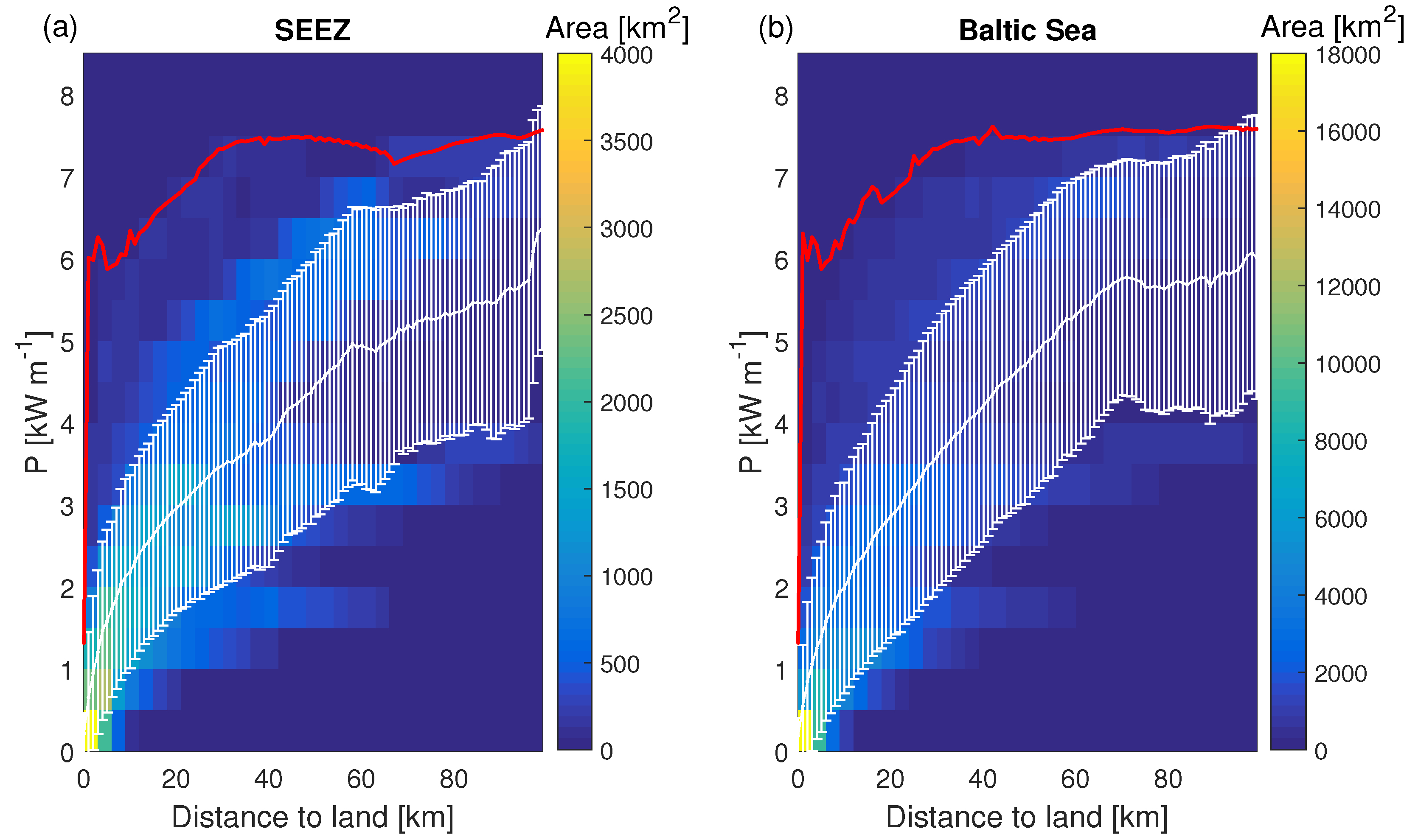
4.4. Dependence on the Distance from the Coastline
The previous maps (
Figure 4 and
Figure 8) show that the distance to the nearest coastline plays an important role in controlling the wave power potential. When the wind is from the coast, the fetch limits the growth of the near-shore waves. For other wind directions, wave energy is smaller than in the open sea because of the sheltering of the shoreline and islands as well as because of the dissipation due to bottom friction and depth-induced wave breaking when the waves approach from open sea to the shallow coastal waters. The influence of these factors on the wave energy is different (see
Figure 8), but there is an overall dependence on the geometrical situation, which to some extent can be quantified by the distance to the nearest coast. For two points given in latitude and longitude, the distance between them can be effectively approximated using a Haversine formula [
48]. This was done for each sea point and all land points on the computational grid.
Figure 9 displays the variation of annual average wave power at different distances from land for the SEEZ in (a) and compares it to the Baltic Sea as a whole in (b). A largely similar pattern can be seen for the wave power, with an increase close to the square-root of the distance from land for at least the first 40 km from the coast.
Figure 9 shows that the wave power resource can vary greatly at the same distance from the coast. The near-shore variation (less than 5 km from the coast) in wave power ranged from nearly zero to about 6.3 kW/m within the SEEZ. At about 30 km from the coast, variations up to about 7.5 kW/m occurred but very few places had less than 1 kW/m wave power as the annual mean. Such variation needs to be further investigated when areas more or less suitable for placement of wave energy converters are to be identified. A mapping using a relative classification for each grid cell could be useful for further investigation including other aspects.
5. Relative Wave Power Resource Classification
It is reasonable to assume that the costs involved in off-shore projects make it useful to find locations that are relatively close to the coast but also have a reasonably high wave power resource [
49]. In a relative classification for the SEEZ, the locations of which are more promising than others with regards to these aspects can be identified. Five classes are defined based on a conditional mean value and its standard deviation of the wave power at different 1 km distance from coast intervals. In a notation with
denoting the mean annual wave power at a given distance interval from the coast and
denoting the corresponding standard deviation (see
Figure 9), the annual average wave power
P is classified for each grid cell using five classes, where 5 is the best.
Class 1 if the wave power resource is low relative to typical at its distance from the coast:
Class 2 if the wave power resource is lower than average relative to its distance, but not as low as the lowest class:
Class 3 if the wave power resource is greater than average, but not above one added standard deviation:
Class 4 if the wave power resource is greater than one added standard deviation, but not two standard deviations:
Class 5 if the wave power resource is greater than two added standard deviations above the mean for the SEEZ:
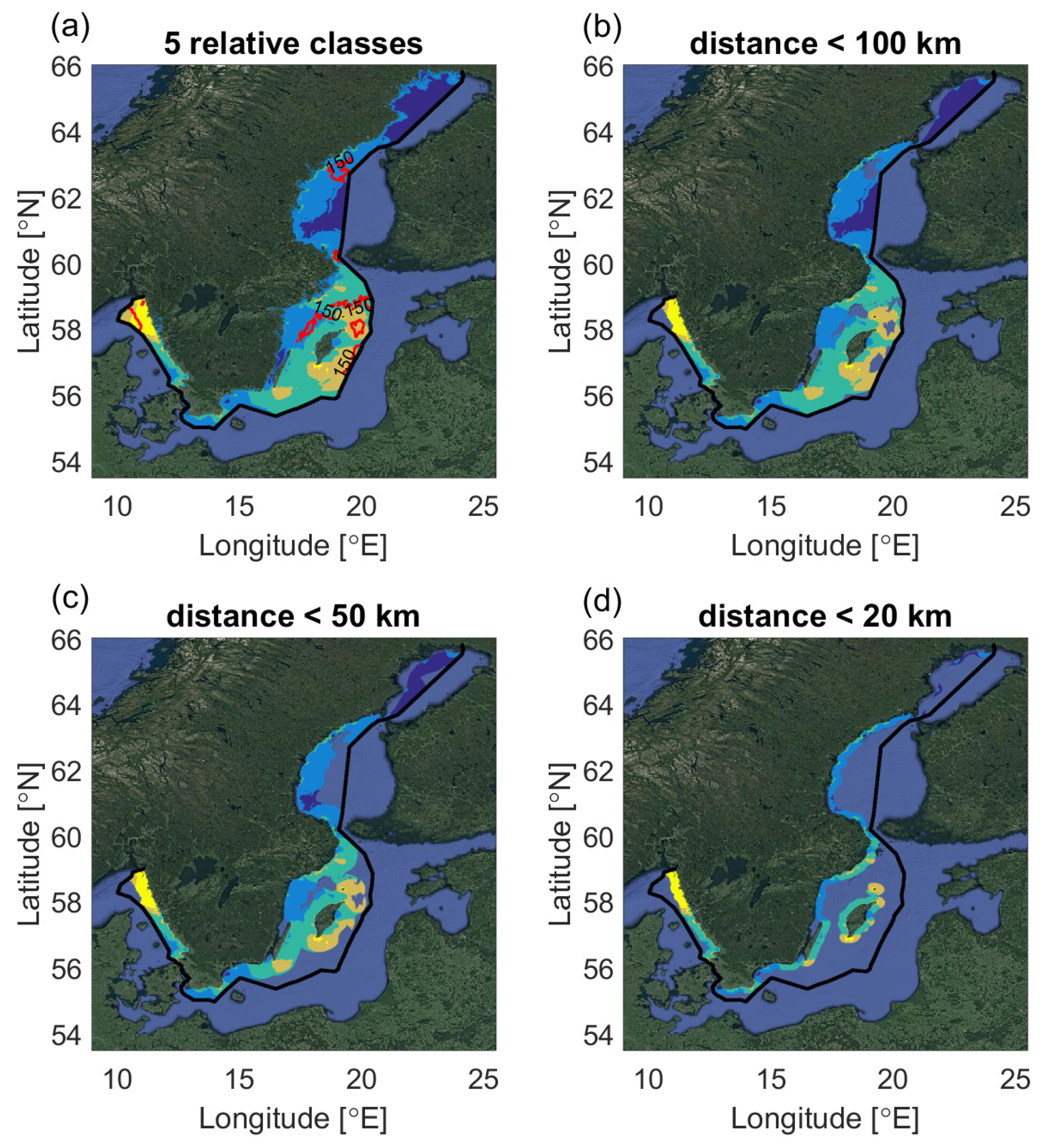
In
Figure 10, a map of the result of this classification is presented. It is noticeable how the lower than average wave power resource classes in blue dominate the results above latitude 60. The main area for class 5 is located on the west coast of Sweden (area 11 in
Figure 5). Other basins show a more diverse range of results.
5.1. Discussion on Additional Aspects
As mentioned in the introduction, locating the best potential wave energy converter sites requires investigations into several aspects. To illustrate the influence of some of these aspects, the 5-class relative resource classification of the previous section is combined with choices regarding water depth, absolute amount of annual mean wave power resource and distance from the coast, and subsequently also a temporal availability aspect.
In
Figure 11a, a red iso-line for a water depth of 100 m is overlaid on top of the relative wave resource classification and it is noticed that several relatively large areas of the SEEZ have depth conditions that exceed 100 m. This is especially true in the outer parts of basins 6, 8 and 11, which are the basins with the highest average wave energy estimates (see
Figure 6). The isoline of 100 m was chosen based on literature about the typical water depth of wave energy converter sites in Europe today [
6], but is not to be interpreted as a limit for commercial installations in the future. The water depth can also affect the efficiency of the WEC if it is bottom mounted and the availability of the site, including the associated costs for divers during placement, operations and maintenance of wave park equipment [
50]. The depth conditions therefore need to be taken into account in a discussion of suitability of potential WEC sites.
The question of choosing a specific amount of wave energy resource that is high enough for a wave energy conversion project to be profitable is a difficult one, as it depends on multiple factors and costs [
49]. In
Figure 11b, a red iso-line for 3.2 kW/m, as a mean value for the SEEZ, has been plotted to illustrate that areas close to coasts within the SEEZ mostly would not have this much wave power resource in the Baltic Sea, but some coastal areas in basin 11 on the west coast of Sweden do. A site near the island of Sicily with an annual average wave power potential of about 3.3 kW/m was discussed in Iuppa et al. [
21] to “… not generate sufficient energy to ensure an economic payback over a reasonable period of time”, but no single wave resource parameter is enough to draw a general conclusion on this. It can, however, be instructive to choose a mid-range value to illustrate a method that can be used to identify interesting areas even if economical concerns and other aspects require additional study.
From the review of Magagna and Uihlein [
6], pilot sites for wave energy converters are typically placed within a distance of about 17 km from the coast. To illustrate the effect of such a choice, a red iso-line corresponding to 20 km distance to resolved land is plotted on top of the relative classification in
Figure 11c. Since wave climate in the Baltic Sea is milder compared to other European coastal regions, a different value might turn out to be appropriate and for commercial wave energy converter sites different choices will likely be applicable. The maps in
Figure 11 should not be considered as final results, but as an illustration of the method. The maximum distance to the shoreline that can be allowed in the Baltic Sea will be determined in upcoming studies, and the maps in
Figure 11 could then be redrawn using this evidence-based value. A strong dependence on distance from the coast exists for the energy losses due to transmission, number of weather windows for O&M (operations and maintenance) activities as well as the presence of extreme significant wave heights. Further study is needed for the Baltic Sea region to determine an appropriate choice for the maximum distance from the shoreline. This will likely also depend on the type of wave energy converter.
Different choices for the different aspects will of course decide how inclusive the identification of potentially interesting sites for wave energy conversion becomes. In
Figure 11d, areas are identified that fulfil the choice of more than 3.2 kW/m as the annual mean wave power and at the same time are located within 20 km of the coastline, and have a water depth of less than 100 m. This identification should be recognized as an interesting case study, but does not imply that other areas could not be of interest, especially for commercial wave energy converter sites.
The regions identified include a large area in basin 11 on the west coast (marked A on the map), which is natural to assume to be one of the best places given its relatively high wave power resource related to long fetch from the North Sea. Some other smaller identified regions include an area south of the island of Öland and southeast of the Blekinge coast near Karlskrona (marked B). There are also regions around the coasts of Gotland (C) and Gotska Sandön (D) as well as a band outside the Stockholm archipelago ranging from close to Sandhamn in the north to Landsort in the south (E) and some minor areas in basin 9.
It should be recognized that some of these locations might not be possible places for offshore infrastructure due to other aspects not discussed here, such as shipping lines, environmental factors and geotechnical assessment of sea floor conditions. As discussed, less strict choices than those made here would give a more inclusive result, which may be considered advantageous since additional aspects will be considered at a later stage. A more inclusive result could, however, also be discussed to identify areas that do not have much wave energy resource, or that are further from the coast, or in deeper water than any existing European WEC project, considering the review by Magagna and Uihlein [
6] from 2015. The relative classification method will also be useful for an inclusive approach, since it will determine whether the locations under consideration have a higher or lower than average wave power resource for their given distance from the coast—a reasonably fair and objective way to find favorable locations for a specific region.
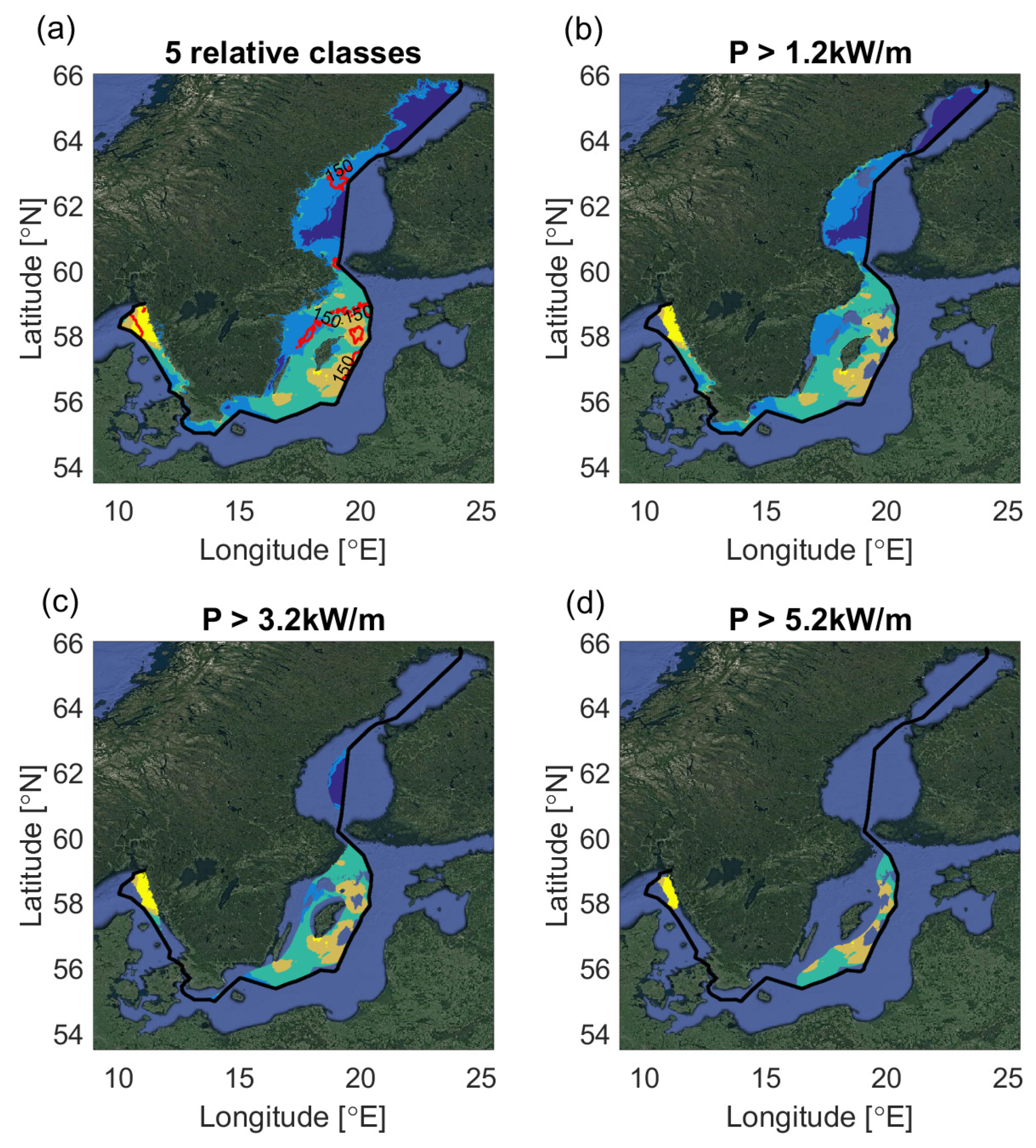
Because choices related to a specific case study can always be discussed in terms of how appropriate they are for a given region, a brief sensitivity analysis in
Appendix C is performed. This includes results for a choice of 150 m water depth and investigations varying the annual wave energy potential between 1.2, 3.2 and 5.2 kW/m, as well as exploring three different choices of distance from the coast at 20, 50 and 100 km.
5.2. Temporal Availability
One topic touched upon in
Section 4.1 is the temporal availability aspect or uneven temporal distribution of the wave energy resource. At these latitudes, the wave energy is largely governed by passing low-pressure systems and associated high wind events may give very high wave energy potentials for short time periods, followed by other times with much lower amounts of wave resource. However, compared to wind, waves generally offer a less intermittent source over time with more predictable forecasting and a higher degree of utility for electric power production [
5,
51,
52].
The cumulative sum of ordered wave power estimates in
Figure 6 showed, however, that a large part of the annual theoretical wave energy potential can come during an amount of time that constitutes only 10 days or a couple of weeks at a basin level.
Figure 12a,b illustrate the same issue but at a kilometer-scale level (or wave energy converter park level) to be able to combine this availability aspect with the other aspects presented. From (a), it is recognized that, for many places, between 40 and 60% of the annual wave energy resource constitute a total time-span of less than 3 weeks per year during the most intense wave events. In (b), similarly, between 70 and close to 100% of the wave energy resource occur during a time-span of less than 3 months, implying long time periods with a low wave energy resource in this region every year. In (c), the relative resource classification is shown with a red overlaid iso-line if 50% of the annual wave energy resource is available during a shorter summed up time than 3 weeks. This shows that, in particular, many coastal regions experience reduced temporal availability (or uneven temporal distribution of the wave energy resource), when significant parts of the year experience low wave resource values.
In the case of wave energy, however, it is also important to mention that fewer occurrences and shorter durations of extreme wave conditions are beneficial for wave energy plant survivability, but these aspects are not studied here. Wave energy converters are also generally designed to generate electricity at the most energetic sea state with regard to the yearly production capability. This will be further covered in an upcoming study within the same Swedish national wave energy resource assessment project [
22].
In
Figure 12d, a zoomed-in view is presented of the southern part of the SEEZ that includes all areas that have passed the introduced criteria in terms of the temporal availability of the wave energy resource, water depth, distance from the coast and amount of wave power resource. The effect added by including the availability aspect was quite small for the previously identified interesting areas in the Baltic Sea (compare
Figure 11d), but had a larger impact for the region denoted A in basin 11 around the coasts and in the northern part. This was interpreted to be related to the wave directional dependence in the northern part of basin 11 where wave energy resource was highest mainly from the southern sector and not as high in the case of waves from the western sector. This implied that although the annual averaged wave power was estimated higher than the average for the SEEZ (3.2 kW/m), this was achieved mainly from high wave power resources associated with a specific directional sector. The wave energy hence became less well distributed over time in parts of basin 11 in comparison to, for instance, in basin 8.
This study presents one approach to account for the temporal availability of the wave energy resource, which is an important consideration when identifying potential WEC sites. Other possible methods to achieve this same goal might include quantifying the seasonal dependence of the wave energy resource [
27]. This aspect will also be covered more extensively in future technical wave energy resource assessments being conducted for the region.
6. Summary and Conclusions
A 16-year wave hindcast dataset at one-kilometer-scale horizontal resolution for the Baltic Sea and Swedish Exclusive Economic Zone was produced using a third-generation wave model, which took seasonal ice-cover into account. This provided the basis for a wave energy resource assessment at a wave energy converter park level, with a typical size of between about 250 by 250 m and 1 . This study also provided the first detailed assessment of the wave power resource for the Baltic Sea region.
The wave hindcast dataset was evaluated against wave buoy measurements within or near the SEEZ and showed a good general agreement with the observations. An overall bias of −0.06 m, centered root-mean-square difference of about 0.26 m and linear correlation coefficient of about 0.92 were found (see
Table 2), which are comparable to other recent third-generation wave modeling efforts. The dataset was noted to have a slightly too large variability for significant wave height, with standard deviation of the significant wave height being between 1 and 10% larger than the observed values for most places.
The theoretical wave power potential was calculated and analyzed for its dependence on aspects such as fetch related to mean wave directional sectors, water depth and distance to coast, presence of sea-ice and temporal availability. Important variations were shown to occur between different geographical basins of the SEEZ, as well as on more local wave energy park scale. When it comes to the temporal availability study of wave power, an important conclusion was that wave energy became less well distributed over time in basin 11 on the Swedish west coast in comparison to basin 8 (in the Baltic proper). These were the two basins showing the highest wave power potentials within the SEEZ and the study shows the importance of considering the directional dependence of wave power in fetch-limited areas. For these areas, the potential annual average wave energy flux reaches about 45 MWh/m/year, but local variations are up to 65 MWh/m/year.
A method to introduce a 5-class relative classification of the wave power resource for the SEEZ region was presented and illustrated using the wave hindcast data. The method effectively compares the amount of wave power resource at a site to other locations at similar distances to the coast, which helps to identify regions that could—from a wave resource perspective—be interesting for further study. The method could be applied to other basins in different parts of the world and contribute at a national level to identify areas for potential WEC sites.
The relative classification was used together with additional aspects such as water depth, distance from the coast and temporal availability of the wave energy resource in a case study to identify some regions that may be of interest for further study as near-shore potential WEC sites. Related work is ongoing within a broad multi-disciplinary project for marine energy conversion that will cover aspects such as environmental factors (including both ecosystem components and nature conservation areas), geotechnical information (e.g., excavation capacity and bearing capacity of the seafloor), variations in sea-level conditions and technical wave energy resource assessment. The identification of potentially interesting sites is illustrated to heavily depend on choices taken for different aspects and this may be best determined at a project level, since economical concerns are also of interest. The datasets and methods introduced here are, however, stepping stones that can be used to pursue overarching goals that are common for wave energy assessments: combining different types of data for identifying and classifying suitable offshore wave energy pilot sites.

 ,
, 


