Assessing the Impact of Cybersecurity Attacks on Power Systems

Abstract

Cybersecurity is an emerging challenge for power systems, as it strongly affects their reliability and the whole energy system cost. The paper uses several Unit Commitments (UC) models, applying different methods to tackle renewables’ uncertainty. The selected power system is IEEE RTS 96. The UC models are used to assess the impact of different cybersecurity threats. The focus is to assess their impact on the total operating cost and the power grid adequacy to handle them. The comparison between the UC models shows that more robust UC models lead to higher total operating costs. The cost, unit dispatching, and energy mix evolution have a non-linear trend, depending on the power system characteristics and the cyberattacks types. However, the paper provides evidence of considerable price signals in the case of the examined cyberattacks. Each Transmission System Operator (TSO) should examine combinations of cyberattacks and operating conditions to identify crucial cases for system stability and power system cost operation. The applied methodology would also require substantial developments or supplementary approaches to assess cyberthreats at the distribution level.

1. Introduction

Power systems are among the most complex and critical infrastructures of a modern digital society, serving as the backbone for its economic activities and security. It is therefore in the interest of every country to secure their operation against cyber risks and threats [1], as stated in the report of the European Commission’s Smart Grids Task Force, as well as in the ‘Cyber Security in the Energy Sector’ report [2] published in 2017 by the Energy Expert Cyber Security Platform (EESCP), stressing the need for addressing the major challenges of cyber threats in the energy sector as well as providing the requirements for addressing appropriately cybersecurity. Potential cybersecurity threats could have cascading effects, leading to damage and power outages, as well as personal data breaches [3].

Over the last few decades, the power system has been modernized. This modernization concerns (i) market aspects, due to its liberalization, (ii) organizational aspects, due to the change of roles from the utilities, where central planning is replaced by decentralized operation with active participation of final consumers, as well as (iii) operational aspects, due to the evolution of smart technologies and communication protocols. Novel Internet of Things (IoT) nodes and smart meters are introduced in various parts of the energy grid, while existing SCADA systems are used for monitoring and control operations that are widely dispersed in case of energy transport and distribution networks. Furthermore, distributed control systems (DCS) are used for single facilities or small geographical areas, while remote terminal units (RTU) and programmable logic controllers (PLC) monitor system data and initiate programmed control activities in response to input data and alerts. 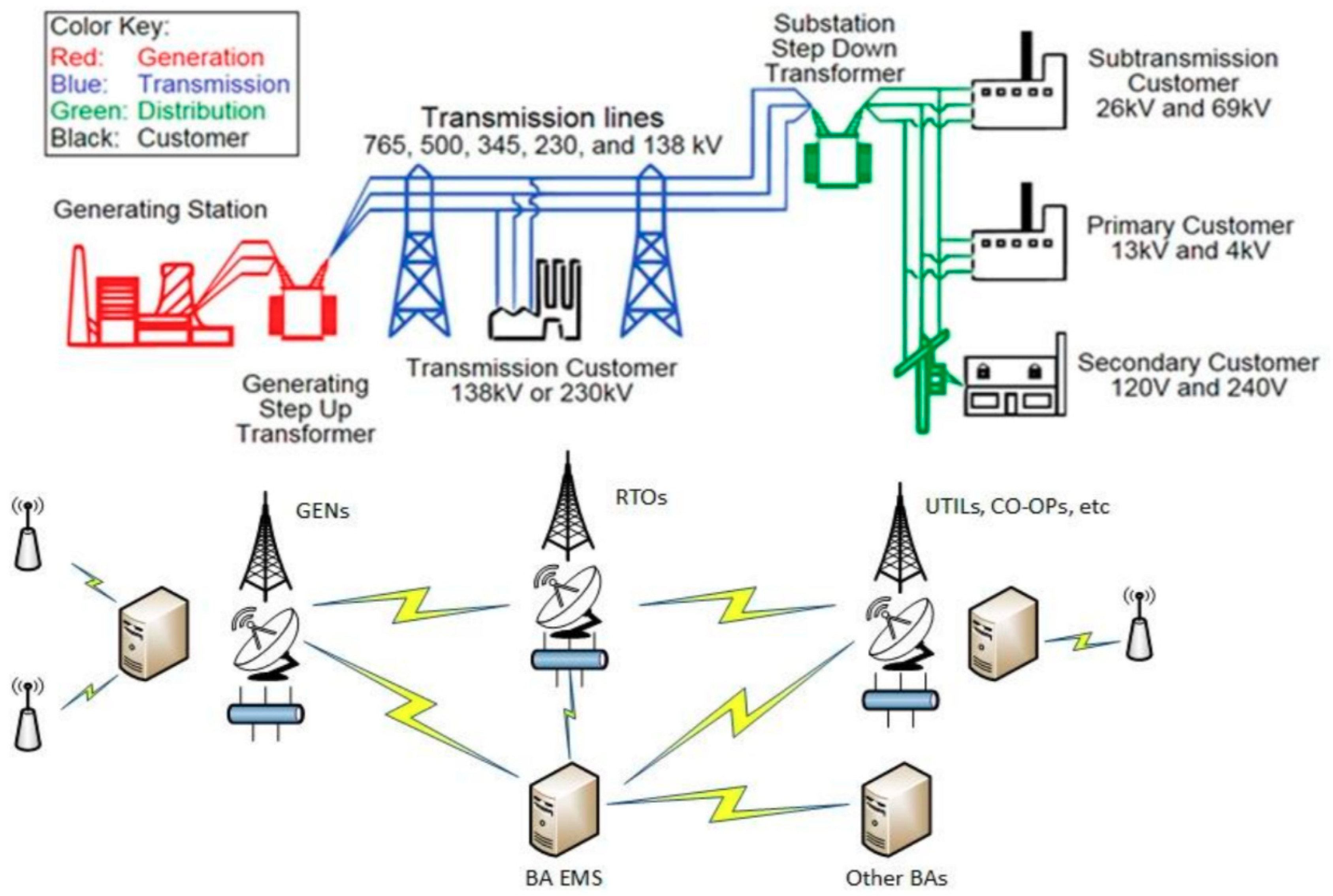Figure 1 provides the typical structure of a modern power system [4], as well as the communication among the different assets of the power system, in generation, transmission, distribution, and consumption.

Cyber threats are evolving at a tremendous pace, exploiting capabilities created by the modernization of the power systems, as stated in the ENISA Smart Grid Threat Landscape report [5]. This is related to the transition from a centralized power system, based on large power stations and vertical integrated utilities, to a decentralized power systems model [6], as well as the complementary evolution of more advanced communication and digital systems. Modern power systems are becoming increasingly dependent on communication systems for their operations, and as a result increasingly susceptible to cyberattacks. As stated in the NIST report for Guidelines for Smart Grid Cybersecurity [7], while integrating information technologies is essential to building the smart grid and realizing its benefits, the same networked technologies add complexity and introduce new interdependencies and vulnerabilities to potential attackers and unintentional errors.

However, the development of smart power systems creates critical challenges, especially related to tackling rapidly evolving cybersecurity issues. This affects the capability of the Transmission and Distribution System Operators (TSOs and DSOs) to guarantee resilience, reliability, stability, security of supply, and power quality for the final users of electricity.

• Essential power system functions at risk from cyberattacks include:
• Electricity supply (generation) stability and reliability;
• Electricity transmission and distribution stability and reliability;
• Communication between systems or equipment;
• Information on the operating conditions of generation, transmission or distribution equipment;
• Black start capability;
• Equipment performance and ability to recover (backup systems).

Cyberattacks could affect not only system operators, but also market participants. For example, demand aggregators create billing systems for issuing invoices to their final consumers. Those systems, either using desktop computers, cloud services, or blockchain technology, are in danger of cyberattacks, which could considerably affect cash flows and finally the viability of market participants. Similar threats exist for participants that use peer-to-peer trading services. Although such types of threats are possible and can have important effect, the threats that affect grid stability are considered more challenging due to their cascading effects.

A crucial issue in the assessment of cybersecurity threats is the identification of their impact on power systems’ reliability and the whole energy system cost. This paper uses different unit commitment models, implementing different levels of robustness to tackle uncertain renewables generation, to assess the impact of the cybersecurity threats on the power systems. It provides price signals on the impact of the threats on the wholesale marginal prices and on the whole energy system costs. It identifies cases where black-out events are inevitable, estimating the overall cost of the interruption in energy service. The paper provides useful insights to the TSOs, as it provides price signals of the cyberthreats, enabling the identification of benchmark values for relevant equipment costs and tariff policies for producers and end users.

Sun et al. [8] provide a review of cyber systems in a smart grid, summarizing the cyber protection and cyber‒physical system testbeds. The paper proposes a methodology for the detection of coordinated cyberattacks, which, however, is not holistic as there are unsolved cyber vulnerabilities that require further research. Mrabet et al. [9] provide a review of the cybersecurity requirements in smart grids, describing different types of severe cyberattacks. The paper proposes a cybersecurity strategy to detect and counter these critical attacks. Jarmakiewicz et al. [10] describe a cybersecurity protection approach for power grid control systems, by identifying key elements of the power system and their importance to power grid security. Shi et al. [11] provide a review of models, methods, and applications for the cyber‒physical interaction in power systems. Poudel et al. [12] present a real-time cyber‒physical system testbed for power system security and control, focusing on voltage stability and generation loss. Hammad et al. [13] present an offline co-simulation testbed for studies of power systems’ cybersecurity and control verification. Liu et al. [14] present a novel model for the evaluation of the validity of active cyber‒physical distribution system. The paper quantifies the impact of cyber faults on functionality validity during distribution automation.

The previous paragraph shows that the literature on cybersecurity issues in power systems is rapidly increasing. However, the papers mainly focus on the identification of security threats, rather than on the assessment on the actual operation and cost of the power systems. There are also a growing number of research papers on specific aspects of the power systems. Part et al. [15] focus on the implementation of cybersecurity strategy for safety systems of nuclear facilities. Gunduz and Jayaweera [16] provide a reliability assessment of a power system with cyber‒physical interactive operation of photovoltaic systems. They present a probabilistic reliability model, concluding that impacts of cyber threats are considerable. However, they do not provide relative price signals but suggest that a relative quantitative assessment is required. Sundararajan et al. [17] provide a survey of challenges and solutions for distributed generation cyber‒physical security. The paper identifies the key vulnerabilities, attacks and potential solutions for solar and wind units at the protocol level. Tellbach and Li [18] examine cyberattacks on smart meters in residential customers, concluding that integrity and confidentiality attacks cause monetary effects on the power grid, while availability attacks—besides monetary effects on the power grid—mainly aim at delaying or stopping the operation of smart meters. Ye et al. [19] provide a quantitative vulnerability assessment of cybersecurity for distribution automation systems. Potential physical consequences of cyberattacks are analyzed at two levels: the terminal device level and the control center server level. A game theory-based approach is used to examine the relationships among different vulnerabilities by introducing a vulnerability adjacency matrix. The results in a relatively small system demonstrate the reasonability and effectiveness of the proposed methodology. Venkatachary et al. [20] provide a review of the economic impacts of cybersecurity in the energy sector. However, the analysis is done in a top-down manner, without applying a detailed robust methodology that assesses the impacts of specific threats to the power system. Liu et al. [21] examine the impact of cyberattacks on the economic operation of power systems. Liu et al. [22] estimate the impact of three different possible cyber events on a physical power grid, using an integrated cyber‒power modeling and simulation testbed. Poudineh and Jamasb [23] examine the impact of electricity supply interruptions in case of the Scottish economy. They provide the sectoral interdependencies as well as the cost of energy not delivered. Considering that those interruptions could result from cyberattacks, the paper provides insights into related price signals.

Cybersecurity is affected by the structure of power systems, as well as by communication protocols and standards. Leszczyna [24] provides a review of standards with cybersecurity requirements for the smart grid. The paper assesses 17 standards, which are described from a cybersecurity requirements perspective and refer to the IEC smart grid architecture. Moreover, the relationships between cybersecurity requirements in different standards are analyzed and visualized. The role of communication standards is important, as shown in a paper that provides a technical overview and benefits of the popular IEC 61850 standard for substation automation [25]. Jarmakiewicz et al. [26] describe a cybersecurity protection approach for power grid control systems. The paper also discusses the verification process of the functionality provided by an implemented cybersecurity system. Cybersecurity is a challenge for different systems and applications, leading to the development of cybersecurity assessment models. A recent paper [27] describes a cybersecurity risk analysis model using fault tree analysis and fuzzy decision theory in order to evaluate cybersecurity risk of particular applications. Zarreh et al. [28] describe a game theory-based cybersecurity assessment model for advanced manufacturing systems. The literature review revealed that cybersecurity in power systems is a challenging issue. Relevant papers are rapidly disseminating; however, they mainly focus on the identification of relevant threats and vulnerabilities, rather than on the quantification of their impact on the power system operation and cost. This gap is the focus of this paper, namely, to provide a quantitative assessment of the impact of cybersecurity threats. Towards providing robust price signals, robust methodologies must be selected. This is the reason that a Unit Commitment (UC) model has been chosen for this analysis. The aim of a UC algorithm is to determine which units will produce energy in each hour of a day to meet demand. The UC problem is complex as it incorporates several techno-economic constraints related to the production units and the transmission lines. The UC problem identifies the power units’ dispatch, considering their operational and maintenance costs, their ramping capacity, their capability to provide ancillary services, and other techno-economic criteria. The UC problem is formulated as a Mixed Integer Linear Programming (MILP) problem, which is adequate to handle such complicated problems. The problem is solved in such a way that the overall fuel cost is minimized with respect to the system’s and unit’s constraints.

The applications of unit commitment models are also extended, as they are considered robust approaches to simulate the power systems operation. UC models examine—in most cases—a national power system or a small power system, providing insights into different challenges it faces. However, to our knowledge, there has been no attempt to quantify the impact of cybersecurity threats on power systems. Moreover, there are few cases providing a comparison among different UC models, which would be a useful step towards revealing the required level of detail for robust solutions and the impact of uncertainties on key variables. The Energy and Environmental Policy laboratory at the University of Piraeus has extensive experience in developing and extending UC models, but its work mainly concerns the Hellenic power system [29,30,31]. Considering that the assessment of cybersecurity threats is a challenging issue, the application of a common power system such as the IEEE RTS 96 with increased penetration of renewables has been selected, as this represents a large but more commonly used power system in the international community. This has led to the application and extension of UC models by the Renewables Energy Analysis Lab at the University of Washington [32].

The paper contributes to the literature by applying different UC models, differentiated by tackling uncertain renewable electricity generation, to estimate the impact of cybersecurity threats in a commonly used power system. The highlights of the paper are: (i) integration of cybersecurity threats in the Unit Commitment problem, (ii) comparison of different UC models on the IEEE RTS 96 power system, tackling differently the uncertainty of renewable electricity generation, (iii) assessment of the impact of cybersecurity threats in the power system cost and scheduling; and (iv) provision of useful insights into the effects of cybersecurity threats on the total operating cost of a power system and its adequacy to handle them.

The rest of the paper is organized: Section 2 provides the methodology applied. Section 3 examines potential cyberattacks on the power system, identifying scenarios that will be described, simulated, and discussed in Section 4. Finally, Section 5 provides the main conclusions and highlights of the paper.

2. Methodology

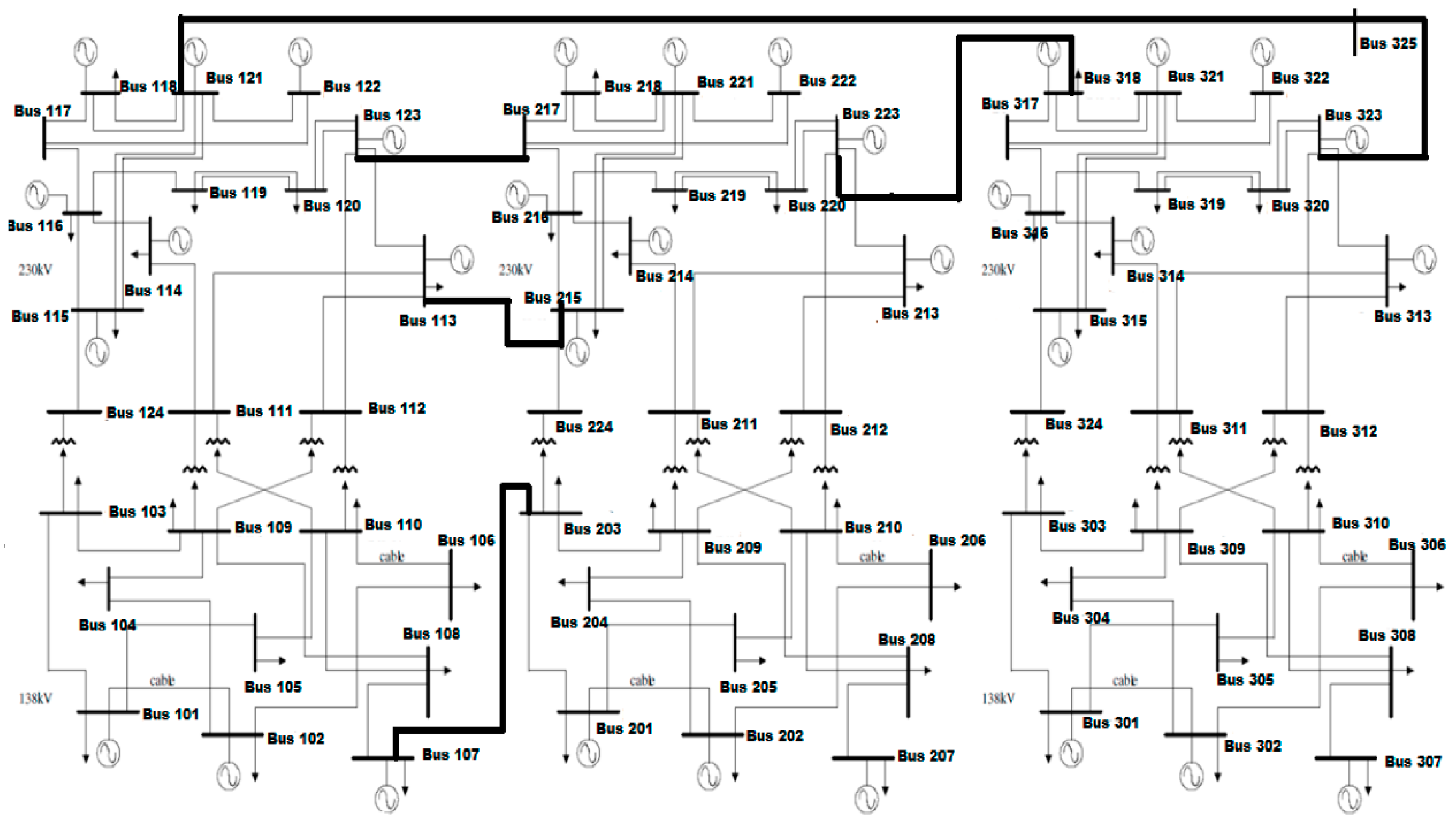
The Renewables Energy Analysis Lab at the University of Washington has developed five different implementations of the Unit Commitment problem [33], where the basic formulation is described in Appendix A. The application of the UC models concerns the IEEE RTS-96 power system, shown in Figure 2. This power system includes, apart from thermal production units of various fuel (nuclear, coal-fired, diesel, natural gas) with 10,215 MW total installed capacity, renewable energy generation units from wind, whose power production is uncertain compared to other renewable technologies such as photovoltaics [33]. The whole system can be seen in the following layout.

Renewable energy sources introduce uncertainty, due to the stochastic nature of the wind and the weather conditions in general. Transmission system operators must forecast the real generation from those renewable sources, affecting the stability of the power system, the strategy of energy market participants. We did not consider other renewable technologies, such as photovoltaics, as their power output can be forecasted with much higher accuracy, so the introduction of photovoltaics would lead to an upgrade of the net load at each bus rather than an introduction of uncertain renewables production. Photovoltaics, aside from the sunset effect, which affects the unit commitment problem and enhances the need for flexible ramping capacity, does not increase uncertainty in the dispatch of power units, as the uncertain power output from wind farms is doing.

The models developed by the Renewables Energy Analysis Lab, used for this paper, are the following: Deterministic unit commitment, Stochastic unit commitment, Improved interval unit commitment, Interval unit commitment, and Robust unit commitment. Each of those models uses a different mathematical procedure to forecast the anticipated renewable production. Some of them are more conservative than others. Consequently, those models are committing more thermal units, and the stability of the system is increased but with a higher total economic cost.

The UC models require a considerable amount of input data, which are described in Appendix B. The modelers have the option to change some constants in the data input program. Through those options, we can modify the penetration of the renewable sources, the variable cost, and ramping capabilities of thermal units, the capacities of the transmission lines, the wind profile and a penalty factor in the case of spilled wind production or unserved loads. In our research, we choose to have 30% of energy from wind power units, which is much higher than the current state of most power grids and a possible future power system of the next decades. Another decision is to go with the unfavorable or favorable wind profile. We have chosen the unfavorable wind profile.

2.1. Differences between the UC Models

2.1.1. Deterministic Unit Commitment Model (DUC)

This model uses only one forecast for the wind production, resulting from the elaboration of historical data. This model provides either conservative or very inefficient solutions in certain conditions. Therefore, the incapability of the model to tackle uncertainty of renewables production, leads to solution with limited robustness.

2.1.2. Stochastic Unit Commitment Model (SUC)

The stochastic model, instead of using a fixed forecast calculates the unit commitment for 10 different wind scenarios, assigning a weight on them based on the probability of each scenario. The model captures a certain level of unhedged uncertainty, which is quantified concerning expected unserved loads and spilled production [34].

2.1.3. Interval Unit Commitment Model (IUC)

This model implements a simplified representation of renewables uncertainty. The deterministic scenario is used a basis, on which an upper and a lower bound scenario for the wind energy production are identified. The model uses upper and lower bound forecasts in order to estimate the ramp-up and ramp-down limits for the thermal units, which leads to the commissioning of more power units and increase of the overall energy cost.

2.1.4. Improved Interval Unit Commitment Model (IIUC)

The Improved Interval Unit Commitment Model (IIUC) is an enhanced version of the previous model, where the upper and lower bounds are replaced by four scenarios. The two new scenarios incorporate more realistic slopes for the ramping capability of the thermal units. This approach is much more realistic because the previous extreme transition values are not possible in the real world. As a result, we anticipate that the IIUC solution will be less expensive than IUC.

2.1.5. Robust Unit Commitment Model (RUC)

The objective function of the model is the following, as presented in [35]:

$${\displaystyle \sum }_{t=1}^T{\displaystyle \sum }_{i=1}^I\left(\alpha ·x_i\left(t\right)+su{c}_i\left(t\right)\right)+max\left\{{\displaystyle \sum }_{b=1}^B{k}_b·g_{i,b}\left(t\right)\right\} \forall t\le T, i\le I$$

(1)

The nomenclature for all UC models are provided in Appendix A. The objective function includes the startup cost and fixed production cost of the power units, as well as the variable production cost in the worst-case scenario, which stands as the main difference with the other models. The model is considered as a conservative unit commitment model with increased robustness, as it is based on the worst-case scenario. The model initially decides which units to be committed, based on their fixed and start-up costs. Then the output power of the power units is calculated to meet the reserves for the worst-case scenario [35].

2.1.6. Comparison of UC Models

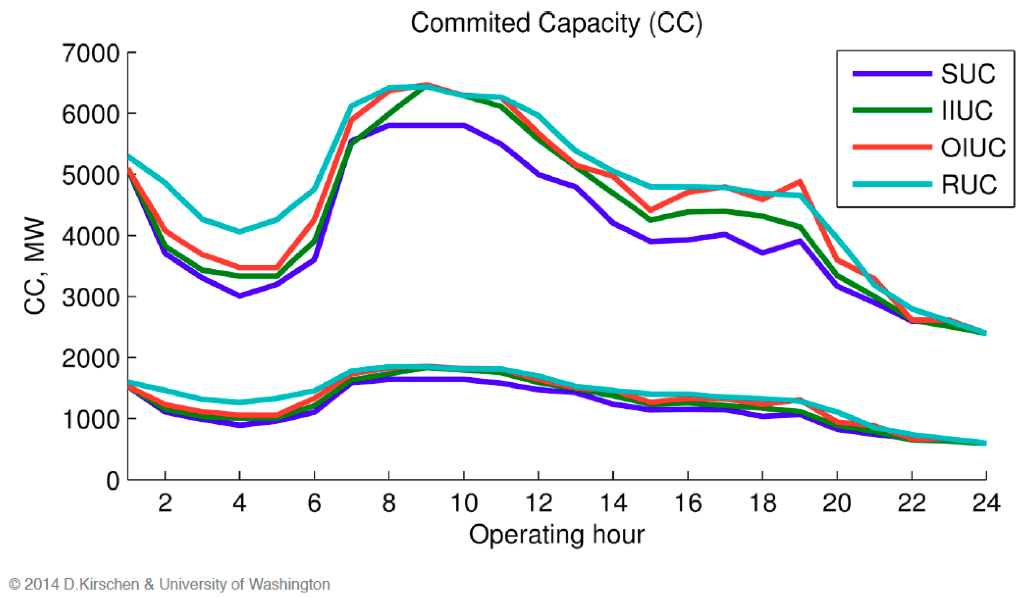
Considering the theoretical model differences, a recent work [36] confirms those results. Figure 3 summarizes the differences between the models. Figure 3 shows that more robust UC models, being more “conservative” in constraints, led to the commitment of more power from dispatching units.

3. Cyberattacks on the Power System

The UC models will be demonstrated on dry-run scenarios of the IEE-RTS96 power system. The prototype will provide a set of different scenarios concerning cybersecurity threats. This section describes potential threats for the power systems. In order to identify the threats, it is important to describe the different Information and Communication Technologies (ICT), integrated within the power systems, with special focus on the TSO, which is responsible for the reliable operation of the transmission system.

Cybersecurity threats affect the capability of the Electrical Power System Operators to guarantee resilience, reliability, stability, security of supply, and power quality to the final users of electricity. Essential system functions at risk of cyberattacks for this demonstration include:

• electricity supply (generation) stability and reliability;
• electricity transmission stability and reliability;
• communication between systems or equipment;
• information on the operating conditions of generation, transmission equipment;
• black start capability.

More specifically, potential cybersecurity threats are:

• smart meters may be used by hackers as entry points into the broader power system;
• unauthorized interference on the measurement of electricity consumption (end-users);
• trip a power-generating unit or modify its schedule;
• cause a blackout in a big area of the grid;
• attack on the electricity market;
• disrupt the proper functioning of the system;
• attacks through the power system on civil infrastructure.

TSOs are responsible for the operation, maintenance, and expansion of the transmission systems. TSOs use Supervisory Control and Data Acquisition System (SCADA) for the high-level process supervisory management of transmission system facilities. SCADA systems are vital for system operators to monitor and control the electricity network. The fact that SCADA/EMS systems are now being interconnected and integrated with external systems creates new possibilities and threats. Those issues have been emphasized in the CIGRÉ joint working groups (JWG) D2/B3/C2.01 and D2.22 [37,38]. As part of the JWG efforts, the various interconnections of a substation were investigated [39]. An emerging challenge of the Transmission System Operators (TSOs) is to identify the vulnerabilities in the power systems, as well as how each cybersecurity threat affects independently and cumulatively those aims. This will help with the design of adequate security measures to ensure a cyber-secure system, which concerns the design of appropriate procedures and policies to tackle each threat, considering the relevant clauses of the ISO/IEC 27032:2012 and ISO 27001 standards.

The power units have installed Remote Terminal Units (RTU), using PLCs for their communication with the system operator. The communication protocols are based on international standards IEC60870-101 and IEC60870-104. The international standard IEC61850, which defines communication protocols for intelligent electronic devices at electrical substations, is an innovative standard, especially as it tackles multi-vendor interoperability [25]. The renewable units’ RTUs communicate through ISDN or PSTN telecommunication services. Distributed generation units, such as photovoltaic units, are usually obliged to install a GSM/GPRS modem for communication purposes, while wind parks have an RTU for their communication with the dispatcher. Although the renewables do not participate in real-time dispatching in the same way with conventional thermal units, due to their stochastic nature, their rapidly growing share raises issues about the scaling-up of potential cybersecurity threats that could affect power systems reliability, security, and overall costs. Therefore, the identification of cybersecurity threats for relevant technologies for the main energy carriers of the future power system, namely natural gas, wind, and solar energy, is an important challenge. The same concerns are relevant in the identification of threats on indicative customers from different consumer types, using different telemetering devices (mainly for billing and profile patterns aims, rather than for dispatching purposes). The structure and communication protocol of power systems identify the potential threats. In case of the evolution of power line communication as a dominant communication method, or the transformation of a power system as an Internet-of-Things place, every device, plug, or connection point of the grid becomes vulnerable to potential cyberattack. This further enhances the importance of cybersecurity as a major challenge for a power system, as the threat is distributed at many levels and points, compared to the top-down consideration of cybersecurity that mainly focuses on attacks on power plants, central control systems, and high-voltage substations. The approach implemented in this paper, using the unit commitment model for assessing cyberthreats, can be robust for tackling top-down threats that affect system stability; however, the consideration of threats in a distributed manner would require considerable model improvements or use complementary approaches to tackle those challenges in more detail.

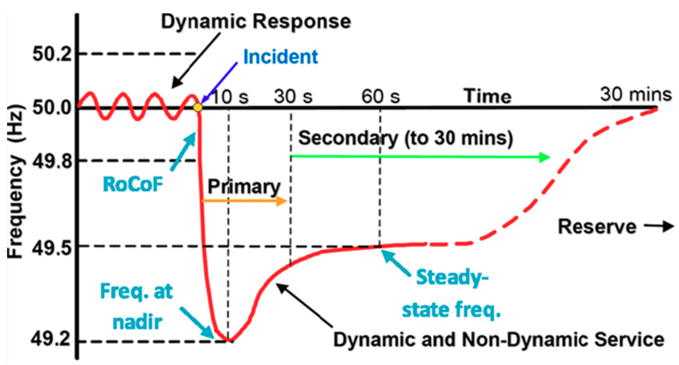
The communication of the thermal power plant with the central dispatching of the TSO is done through special software, called Real-Time Dispatching (RTD), providing instruction every 5 min, and the Automatic Generation Control system (AGC), which enables the provision of the required ancillary services in seconds, as depicted in Figure 4. The thermal units also have a Digital Control System (DCS), which provides several checks concerning its operation and communication with the substation and the dispatching center.

Several types of cyberattacks can take place. This work focuses on attacks on big plants that are dispatched by the Transmission System Operator (TSO), monitored through SCADA systems, and linked to the TSO-operated Automatic Generation Control system (AGC). The examined scenarios are described and discussed in the next section.

4. Results and Discussion

This section provides the results from the simulations. The examined scenarios focus on providing a comparison among the different UC models and secondly on the comparison among the different cybersecurity attacks.

Firstly, the different UC models have been run without any cyberattack, leading to baseline scenarios, entitled DCU_BAS, SUC_BAS, IIUC_BAS, and RUC_BAS for the deterministic, stochastic, improved internal, and robust UC models, respectively.

Secondly, we examined a Cyberattack 1 case with cyberattacks on three thermal units, 400 MW each, so 1200 MW in total. All three units have been scheduled to operate with the baseline scenarios, while the cyberattack was set to take place in the first hour of day, not enabling those units to operate for the whole examined day. A comparison among the first and second set of scenarios enables the provision of price signals on the cost of cyberattacks, as well as a comparison among the different UC models, incorporating a different level of robustness for tackling the stochastic and uncertain nature of the renewables.

Thirdly, another set of scenarios was examined using the RUC model, which is a robust model enabling the provision of price signals in cases where the transmission system operator (TSO) adopts a more conservative approach toon tackling uncertainties in the power system. This set of scenarios, Cyberattacks 1–4, examines different cases of cyberattacks. More specifically, the following cyberattack cases where examined: (1) cyberattacks in three thermal units, with 1200 MW total capacity, (2) cyberattacks in six thermal units, with 2400 MW total capacity, (3) cyberattacks in three wind farms, with 1200 MW total capacity, (4) cyberattacks in three thermal units, of 1200 MW, and three wind farms, of 1200 MW, with 2400 MW total capacity. In all cases, the thermal units and wind farms were scheduled to operate in the baseline scenarios. 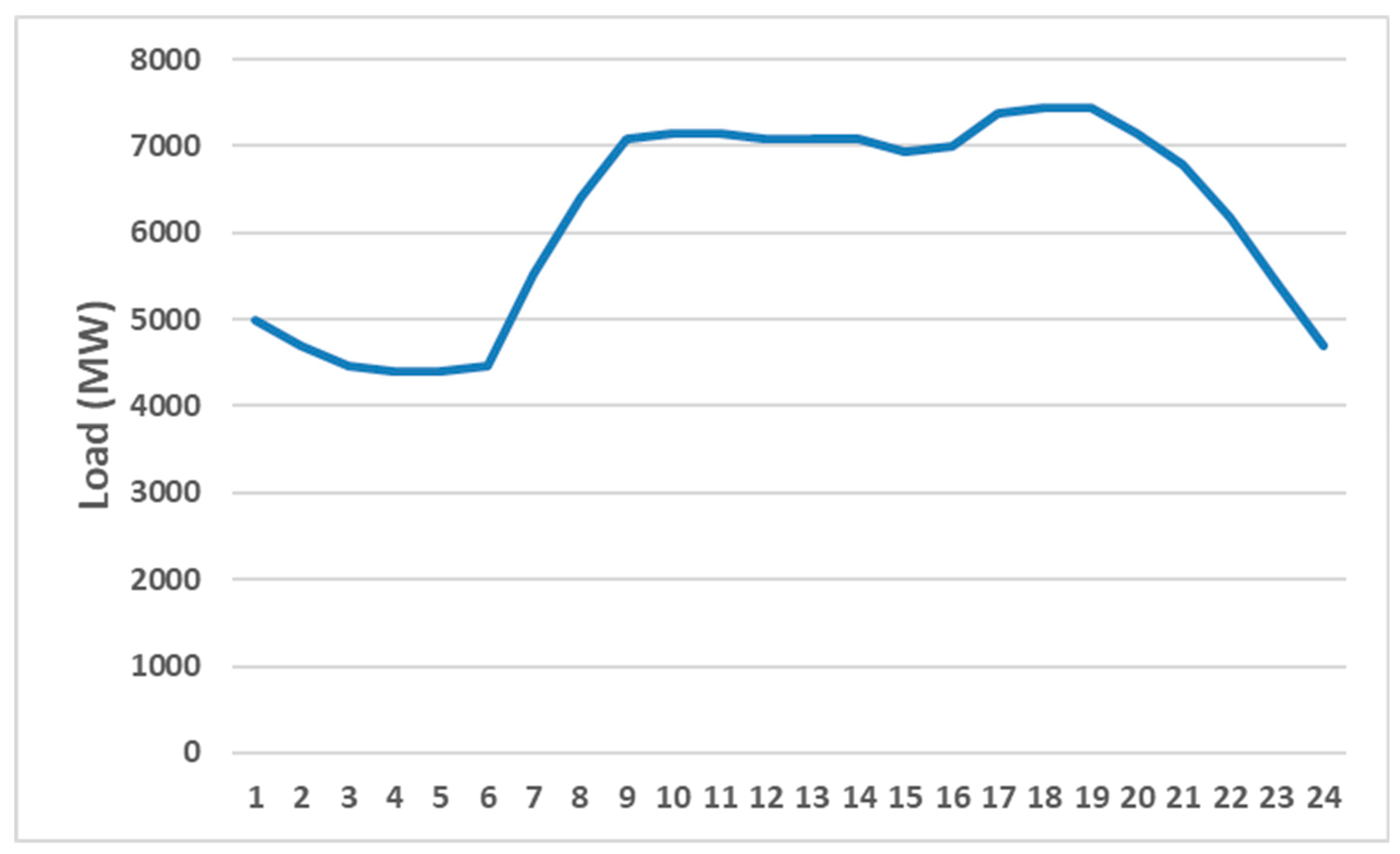Figure 5 provides the evolution of hourly demand in the examined day, deviating between 4.3 and 7.4 GW.

Therefore, the examined cybersecurity attacks concern a considerable share of the generating capacity that is unable to meet the load. However, the examined system has 10.2 GW installed thermal plants, as well as 6.9 GW of wind farms; therefore, the examined cyberattacks are crucial to the power system stability and operating costs, but there is still spare capacity, with flexible ramping capability to meet such events. However, considering that the cyberattacks take place on dispatched thermal and RES plants, those attacks lead to increased operating costs, due to a change in the energy mix, as well as to start-up and shutdown costs for switching off the cyberattacked units and switching on new and more expensive units.

Table 1. Objective function cost (in USD) for different scenarios.

	Objective Function Cost
DUC_BAS	1,019,770
SUC_BAS	2,056,180
RUC_BAS	2,056,184
DUC_Cyber1	1,276,210
SUC_Cyber1	2,548,230
RUC_Cyber1	2,423,626
RUC_Cyber2	2,952,878
RUC_Cyber3	2,207,915
RUC_Cyber4	2,548,225

shows the evolution of the overall cost, as optimized in the objective function. The comparison among the different models shows that the incorporation of more technical constraints, as in the robust and stochastic models, compared to the deterministic solution, leads to a considerable increase in the cost. Through the implementation of the cyberattacks—in the case of Cyberattack 1 scenario, with attacks on three thermal units—the cost is further and considerably increased for all scenarios, especially for the stochastic and robust UC models. Results are from the interval UC models, as those models experienced difficulty in finding feasible solutions. The examined scenarios have also led to a considerable increase in the total computational time, especially in the case of the stochastic UC model. This has led the author to increase the convergence gap, which has led to a possible local minimum solution, rather than a global optimum, as can be seen in the increased cost compared to the robust UC model.

We further focused on the RUC model, examining different cyberattacks’ scenarios. Table 1 shows that cyberattacks on thermal plants lead to considerably higher costs compared to attacks on wind plants. This is attributed to the fact that the attacked thermal plants were set to operate at their nominal capacity, due to their comparable cost, constituting base load plants. The enforced switching-off of those units, with a high capacity factor compared to renewables, led to the need for dispatching further units, as well as increasing the operation of more expensive units. Dispatching of units does not take place only for generating purposes, but also for providing the requested ancillary services for the system stability. Especially in more robust UC models, such constraints lead to higher costs, as shown in Table 1, where Cyberattack 1, in the case of the deterministic model, is considerably less costly compared to the robust and stochastic UC models.

Table 2. Number of thermal units dispatched for different scenarios using the RUC model.

	Units Committed
	RUC_BAS	RUC_Cyber1	RUC_Cyber2	RUC_Cyber3	RUC_Cyber4
1	30	27	26	31	29
2	11	12	17	16	16
3	9	10	17	13	15
4	7	12	15	8	13
5	7	15	16	10	14
6	14	20	23	15	20
7	31	32	41	32	36
8	35	44	45	41	42
9	42	46	46	42	47
10	43	46	53	43	47
11	43	48	58	45	48
12	43	46	51	43	47
13	43	46	53	43	46
14	43	46	56	43	46
15	43	46	52	43	46
16	43	46	53	43	46
17	44	46	56	46	47
18	45	50	56	46	47
19	47	56	64	46	49
20	45	46	51	46	47
21	34	44	45	38	44
22	25	28	36	26	30
23	11	17	21	21	23
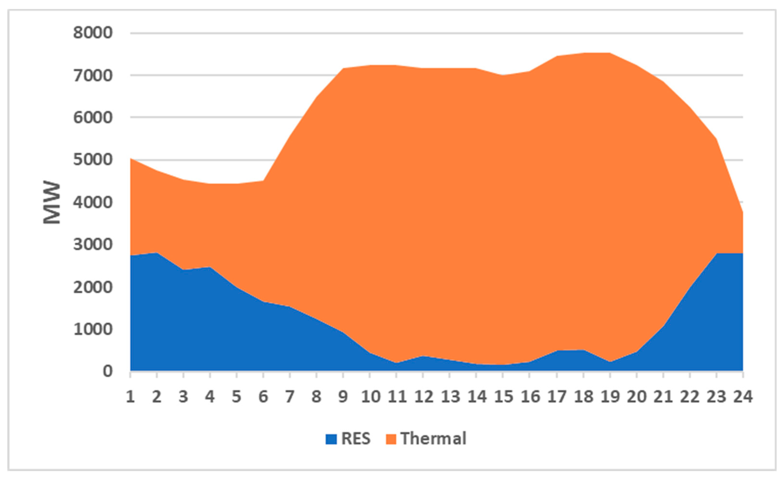
24	7	7	12	9	13

shows that different cyberattacks affect the dispatched units, leading to a different number of units that operate each hour. The importance of thermal plants is depicted in Figure 6, which shows the limited power generation from wind plants, which can justify the limited effect on the operational cost, compared to the thermal plants. However, in the case of different renewables generating profile, i.e., with photovoltaics that operate at peak hours with a high capacity factor and create a sunset effect, cyberattacks on their inverters could lead to considerable ramping needs.

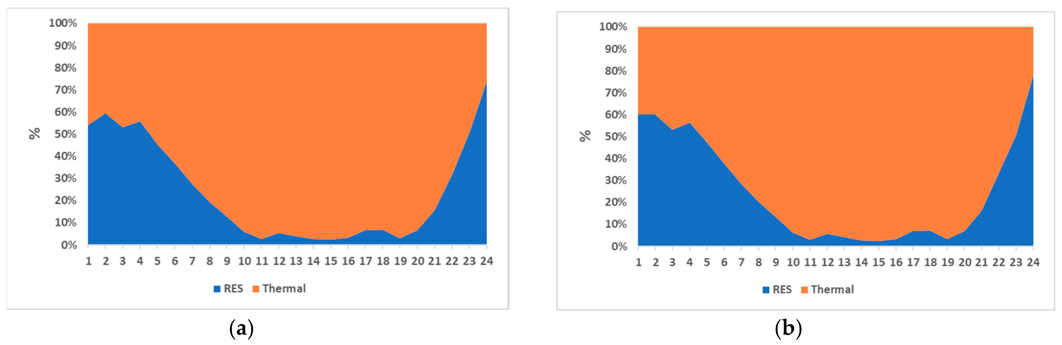
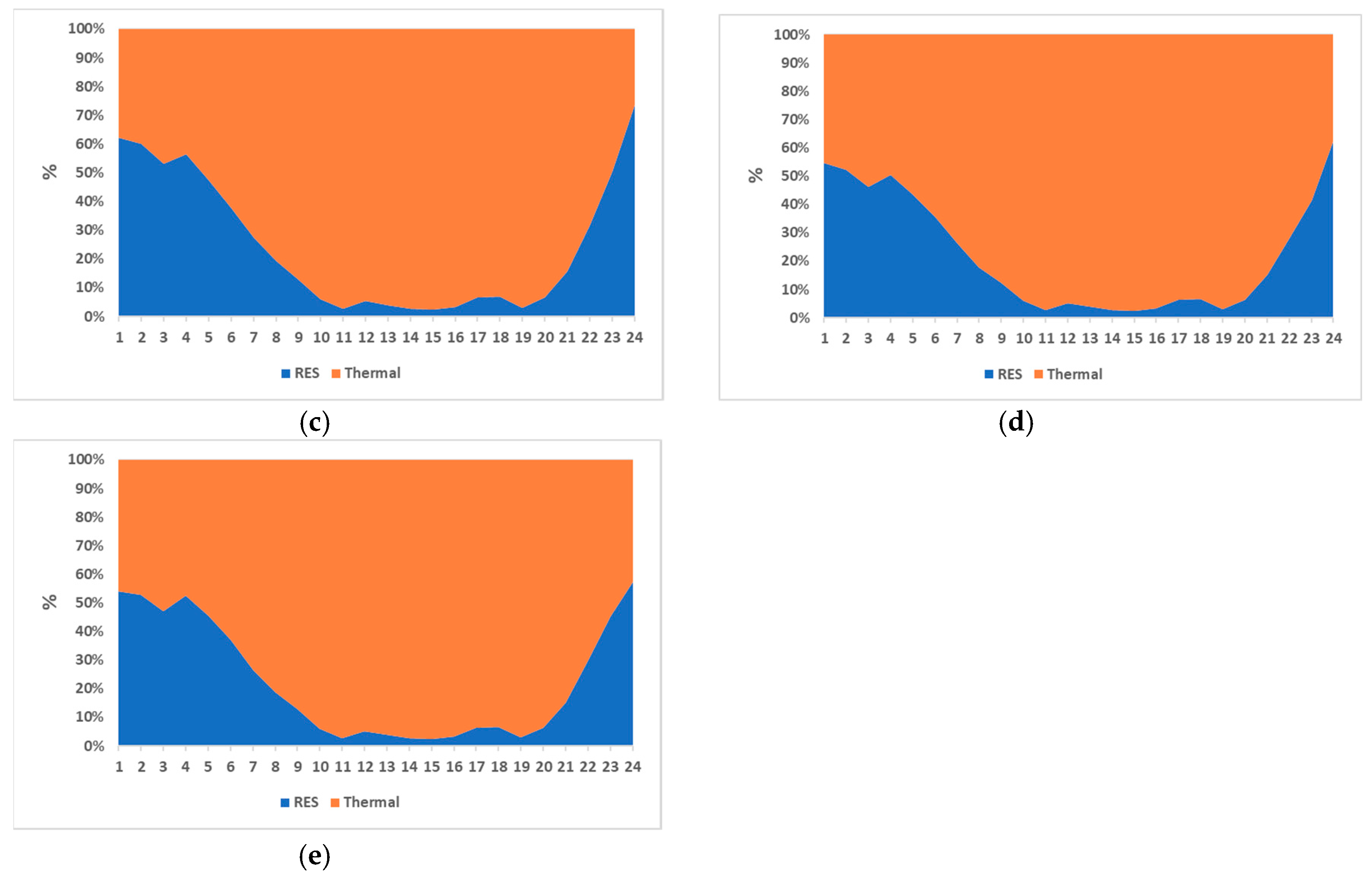
Therefore, cyberattacks on thermal units affect both start-up and shutdown costs, as well as generating and ancillary services costs. However, we cannot provide a generic conclusion that cyberattacks always have a higher impact on total operating costs, as renewables have a low operating cost, and therefore the decommissioning of those units might lead to a more expensive energy mix. However, the examined cases quantitate a higher impact on attacks on thermal units. Moreover, the examined cases using the RUC model show that they also affect the energy mix,—not only the dispatching of thermal plants but also the curtailment of wind plants. This is depicted indirectly in

Table 3. Energy mix for different scenarios with the RUC model.

	RUC_BAS	RUC_Cyber1	RUC_Cyber2	RUC_Cyber3	RUC_Cyber4
RES	20.20%	21.29%	20.63%	19.52%	19.83%
Thermal	79.80%	78.71%	79.37%	80.48%	80.17%
Total	100.00%	100.00%	100.00%	100.00%	100.00%

, which shows that the energy mix is changed as the curtailment of wind production changes. This can also be seen in Figure 7, which shows small but evident changes in the energy mix. However, those changes also depend on the topology of the network, the nodes of the cyberattacked units, their operating condition, and the interconnections among different nodes. Therefore, the operating cost, unit dispatching, and energy mix evolution show a non-linear trend on the effect of different scenarios. A clear outcome from the analysis is that each TSO should examine different combinations of cyberattacks with different operating conditions to identify cases that are more crucial for the system stability and the overall power system cost operation. The examined attacks show an increased cost for the power system operation and reveal the importance of base load plants. However, in the case of power system operation in marginal conditions, namely with limited available capacity, the importance of flexible units with high ramping capacity might be more important.

5. Conclusions

This paper aims at assessing the impact of cybersecurity attacks on power systems. It uses different mixed-integer linear programming unit commitment models, which apply different methodologies to incorporate high levels of renewable energy production. The UC models, applying different methods to integrate the uncertainty from the renewables, are further extended to integrate cybersecurity threats, aiming to compare the UC models but also the effect of cybersecurity threats on different power capacity mixes and reliability uncertainty. Our focus is on the effects on the production side, hence the total operational cost, the average energy cost, the dispatch of power units, as well as the power grid adequacy to handle the cybersecurity threats. The selected power system is IEEE RTS 96.

The examined scenarios focus on providing a comparison of the different UC models and the different cybersecurity attacks. The comparison between the UC models confirmed our theoretical assumptions that more robust UC models mean higher total operating costs, due to the more conservative approach to tackle uncertain renewable electricity generation and the consideration of ancillary services. The examined cyberattacks take place on dispatched thermal and RES plants, leading to increased operating costs. This is attributed to the commissioning of more expensive units as well as the increased start-up and shutdown costs, due to the switching on new and more expensive units and the switching off the cyberattacked units. Moreover, the scenarios lead to an increase in the total computational time for finding the optimum solution. The results show that cyberattacks on thermal units affect both start-up and shutdown costs, as well as generating and ancillary services costs, leading to a higher impact compared to attacks on wind plants. However, the paper cannot provide a generic conclusion that cyberattacks on thermal plants always have a higher impact on total operating costs, as renewables have a low operating cost, and therefore the decommissioning of those units might lead to a more expensive energy mix.

The effects depend on the topology of the network, the nodes of the cyberattacked units, their operating condition, the interconnections among different nodes, and the ramping capacity of the available units. The cost, unit dispatching, and energy mix evolution have a non-linear trend that depends on the power system characteristics. The examined cases lead to considerable price signals on the potential effects of cyberattacks. However, each TSO should examine different combinations of cyberattacks in different operating conditions to identify cases that are more crucial for the system stability and the overall power system operational costs. The approach implemented is useful for assessing cyberattacks at a system level. However, unit commitment modeling cannot quantify threats at the distributed level, unless considerable model developments are made and/or more detailed approaches are elaborated. This creates challenges for further research at the distribution level, which could be scaled up to be integrated at system level.