Article

Bayesian Estimation on Load Model Coefficients of ZIP and Induction Motor Model

1
State Grid Jiangsu Electric Power Company Ltd., Nanjing 210008, Jiangsu, China
2
GEIRI North America, 250 W Tasman Dr. STE 100, San Jose, CA 95134, USA
*
Author to whom correspondence should be addressed.
Energies 2019, 12(3), 547; https://doi.org/10.3390/en12030547
Submission received: 15 January 2019 / Revised: 2 February 2019 / Accepted: 2 February 2019 / Published: 11 February 2019

Abstract

:
Parameter identification in load models is a critical factor for power system computation, simulation, and prediction, as well as stability and reliability analysis. Conventional point estimation based composite load modeling approaches suffer from disturbances and noises, and provide limited information of the system dynamics. In this work, a statistics (Bayesian Estimation) based distribution estimation approach is proposed for both static and dynamic load models. When dealing with multiple parameters, Gibbs sampling method is employed. The proposed method samples all parameters in each iteration and updates one parameter while others remain fixed. The proposed method provides a distribution estimation for load model coefficients and is robust for measuring errors. The proposed parameter identification approach is generic and can be applied to both transmission and distribution networks. Simulations using a 33-feeder system illustrated the efficiency and robustness of the proposal.

1. Introduction

1.1. Composite Load Modeling Methods

Load modeling is a traditional topic in power systems and has been widely studied over the years [1,2,3,4,5,6,7,8]. The importance of an accurate model for voltage stability studies is established in [9]. In [10,11], the authors discussed load modeling in the context of planning, operation, and control systems. The emergence of smart grid technologies, such as distributed generation (DG) and load/demand side management, has created the need for appropriate load models in order to further improve the accuracy and reliability of the power system [12,13].
Load models can be categorized into static models and dynamic models. Static models include the ZIP (constant impedance (Z), constant current (I), and constant power (P)) model, the exponential model, and the frequency dependent model. Examples of widely used dynamic models include the induction motor (IM) and the exponential recovery load model (ERL) [1]. The research focus to date has been on composite load modeling, which consists of static and dynamic models [1]. Specifically, in [1], it is shown that the ZIP+IM model can be used under various conditions and in different locations and compositions. A simplified composite model is shown in Figure 1.
Component-based and measurement-based approaches are two typical load model parameter identification methods that are used today [11,14]. The component-based approach requires information of load compositions. As introduced in [1], this approach requires models of individual components, component compositions (consumption of different load type in percentage), as well as class composition (residential, industrial or commercial load percentage). Measurement-based approaches calculate the parameters using algorithms such as least-squares (LS) and genetic algorithm (GA) based on selected model structure by minimizing the objective function as follows.
min 1 n i = 1 n [ ( P i m P i e ) 2 + ( Q i m Q i e ) 2 ]
where superscript “m” indicates the measured value, and “e” presents the estimated value. Measurements should be obtained under different conditions and disturbances. Different techniques have been used in [14,15,16] to identify the parameters for the composite model. Additional methods for load model parameter identification include the Hammerstein model based on real-time system identification for dynamic load [17] and the artificial neural network (ANN), which is based on modeling proposed in [18].

1.2. Motivations for Using Bayesian Estimation

Traditional measurement based parameter estimation approaches do not consider the robustness of the model, and therefore the model sometimes may fail to present the characteristic of the load accurately due to its time-varying feature. Thus, in [19], the robust time-varying load parameter identification approach uses batch-model regression to obtain the updated system parameters. Moreover, the measurement based approach is highly dependent on measurements from meters, and so measurement anomalies may affect the robustness of the estimations in both time-varying and time-independent load models. Influence of measurement noises when implementing various parameter identification methods is an issue discussed in [20]. The challenges in component based approaches are that they rely on individual load components and the compositions of these load. In [4], for example, ZIP coefficients, commonly used in electrical appliances, have to be first determined in order to develop an accurate model and before critical values can be applied. Moreover, the process of determining different components involves such factors as characterization of consumers, clustering, and weather. Since the data are highly dependent on the type of day, weather, and service class, it is a computationally wasted approach to get ZIP coefficients for these appliances. Difficulties involved in obtaining the comprehensive load composition information is another fact that needs to be carefully considered when implementing component based approaches.
Bayesian estimation (BE) based composite load parameter identification approach, on the other hand, can successfully overcome the aforementioned disadvantages in measurement-based and component-based approaches. First, BE is a time-varying estimation method. Parameters can be updated according to the requirements. Second, BE does not require the complicated procedure used in component based approaches. The information of the composition of the loads and the coefficients of the appliances are not necessarily needed. Third, BE is a robust estimation method due to its statistic characteristics: measurement anomalies will not significantly affect the results if the number of samples is large enough, and the measurement error will not affect the estimation results since in each step of sampling the estimated parameter is drawn from a posterior distribution calculated according to the data and eventually forms a distribution of the target parameter.

1.3. Bayesian Probability and Gibbs Sampling

Bayesian probability is one of several interpretations of probability theory. To evaluate the probability of a hypothesis, Bayesian probability specifies some prior probability, which is then updated to a posterior probability in the light of new, relevant data (likelihood). The formula of Bayesian estimation can be written as:
p ( θ | x ) = p ( θ ) · p ( x | θ ) p ( θ ) · p ( x | θ )
where p ( θ ) is the prior, p ( θ | x ) is the posterior given a observation x, and p ( x | θ ) is the likelihood. The denominator is called the normalization factor. Bayesian estimation gives the probability density function (PDF) of a parameter, which is given by some already known observations. It is the product of the combination of prior information as well as observations of happened events (likelihood). Different from a specific number given by ML, a PDF is able to provide more information and can be used in such functions as forecasting and optimization.
Gibbs sampling is an extension of the Monte Carlo Markov Chain method [21], which performs well when there are multiple parameters to identify. Following the principle of Bayesian probability, Gibbs sampling calculates the posterior distribution of one parameter while fixing the value of others. Then, a new sample of the target parameter is drawn from the posterior, and the next new parameter is sampled with the updated sample. The detailed sampling algorithm is shown in Algorithm 1.
Algorithm 1 Gibbs sampling.
  • Get measurement of x .
  • Draw initial samples θ ( 0 ) q ( θ ) , where q ( θ ) is the prior and θ = { θ 1 , θ 2 , , θ M } .
  • For iteration k = 1 , 2 , , K
    • Calculate p ( θ 1 | θ 2 ( k 1 ) , θ 3 ( k 1 ) , , θ M ( k 1 ) , x ) and draw sample θ 1 ( k ) ,
    • Calculate p ( θ 2 | θ 1 ( k ) , θ 3 ( k 1 ) , , θ M ( k 1 ) , x ) and draw sample θ 2 ( k ) ,
    •  ⋮
    • Calculate p ( θ M | θ 1 ( k ) , θ 2 ( k ) , , θ M 1 ( k ) , x ) and draw sample θ M ( k ) .
    End For
  • The distribution estimate is the histogram of θ k , k = K ̲ , , K , where K is the preset maximum iteration number, and K ̲ is the burn-in number. The results θ k , k = 1 , , K ̲ 1 , are burn-in data and discarded.

1.4. Summary of Contributions

The following contributions are made in this work.
  • To the best knowledge of the authors, the proposed Bayesian approach has not been investigated in the context of load model identification. Bayesian estimation-based approaches have been used in wind forecasting and state monitoring [1,2,22], as well as load forecasting [3,4,5]. The promising performance has shown plentiful possibility in power systems.
  • The proposal is a generic approach. Detailed formulation and derivation of both static (ZIP) and dynamic (IM) models are presented. The proposed algorithm can be applied in both transmission and distribution network context.
  • Numerical experiments illustrated that the proposal provides robust distribution estimation despite the existence of noise. Furthermore, the proposal estimation is more accurate in point estimation than conventional algorithms.
The rest of the paper is organized as follows. In Section 2, a ZIP model for steady state is presented, and the Gibbs sampling is derived. In Section 3, an induction motor model in the context of dynamic state is presented. A modified version of Gibbs sampling is proposed. Numerical experiments are presented in Section 4 to illustrate the effectiveness and robustness of the proposed algorithms. Section 5 discusses existing difficulties in applying the proposal to the real-time operation. Section 6 concludes the paper.

2. ZIP Model and Coefficient Estimation

2.1. ZIP Model

The ZIP model describes how the power of load changes as voltage varies in the steady-state condition. The ZIP model is presented as follows.
P = P 0 ( α 1 V ¯ 2 + α 2 V ¯ + α 3 ) , Q = Q 0 ( α 4 V ¯ 2 + α 5 V ¯ + α 6 ) , i = 1 3 α i = i = 4 6 α i = 1 ,
where V ¯ = V V 0 , P and Q are real and reactive power, and V is voltage magnitude at the load terminal. Variables P 0 , Q 0 and V 0 represent the values of the respective variables under the initial operating condition. When voltage V deviates from V 0 , real and reactive power of the load are assumed to follow a quadratic model. As the real power and reactive power follow the same form of model, we discuss only the real power as an example in the following. The identification of reactive power parameters follows the same procedure.
Define y [ t ] = P [ t ] P 0 , x [ t ] = V [ t ] V 0 , where P [ t ] and V [ t ] are the tth measurements of the real power and voltage magnitude of the ZIP load. The following assumptions are made.
  • The measurement noise follows a normal distribution, i.e., y [ t ] = α 1 x [ t ] 2 + α 2 x [ t ] + α 3 + ε [ t ] , where ε [ t ] N ( 0 , 1 / τ ) , and 1 / τ is the variance The reasons for making this assumption are: (1) According to the law of large numbers, a normal distribution would be the best one to represent the characteristics of the noise if the number of experiment is large enough. (2) Since normal distribution is a conjugate distribution, it is easier for model parameter updating when implementing Gibbs sampling.
  • Total number of n independent and identically distributed (i.i.d.) samples are drawn, namely ( x , y ) { ( x [ 1 ] , y [ 1 ] ) , , ( x [ n ] , y [ n ] ) } . Thus, the likelihood is
    p ( x , y | α 1 , α 2 , τ ) t = 1 n exp [ ( y [ t ] μ [ t ] ) 2 τ / 2 ] ,
    where μ [ t ] α 1 x [ t ] 2 + α 2 x [ t ] + 1 α 1 α 2 is the mean.

2.2. Gibbs in the ZIP Model

Gibbs sampling can be directly applied in the ZIP model estimation. Assume the prior distributions are as follows.
α 1 N ( μ 1 ( 0 ) , 1 / τ 1 ( 0 ) ) ,
α 2 N ( μ 2 ( 0 ) , 1 / τ 2 ( 0 ) ) ,
τ G ( a ( 0 ) , b ( 0 ) ) .
where the distribution of τ is a gamma distribution follows G ( a , b ) . It can be shown that, after each iteration of Gibbs sampling, the post distributions of these three parameters remain in the same form. Gibbs sampling of the ZIP model is stated in Algorithm 2. The detailed derivation of the algorithm can be found in Appendix A.
Algorithm 2 Gibbs Sampling in the ZIP model.
  • Get measurement of x , y .
  • Draw initial samples α 1 N ( μ 1 ( 0 ) , 1 / τ 1 ( 0 ) ) , α 2 N ( μ 2 ( 0 ) , 1 / τ 2 ( 0 ) ) , τ G ( a ( 0 ) , b ( 0 ) ) .
  • For iteration k = 0 , 1 , 2 , , K
    • Draw a sample α 1 ( k + 1 ) N ( μ 1 ( k + 1 ) , 1 / τ 1 ( k + 1 ) ) , where
      μ 1 ( k + 1 ) τ 1 ( k ) μ 1 ( k ) τ ( k ) t = 1 n ( α 2 ( k ) 1 α 2 ( k ) x [ t ] + y [ t ] ) ( 1 x [ t ] 2 ) τ 1 ( k ) + τ ( k ) t = 1 n ( x [ t ] 2 1 ) 2 , τ 1 ( k + 1 ) τ 1 ( k ) + τ ( k ) t = 1 n ( x [ t ] 2 1 ) 2 ,
    • Draw a sample α 2 ( k + 1 ) N ( μ 2 ( k + 1 ) , 1 / τ 2 ( k + 1 ) ) , where
      μ 2 ( k + 1 ) τ 2 ( k ) μ 2 ( k ) τ ( k ) t = 1 n ( α 1 ( k + 1 ) 1 α 1 ( k + 1 ) x [ t ] + y [ t ] ) ( 1 x [ t ] ) τ 2 ( k ) + τ ( k ) t = 1 n ( x [ t ] 1 ) 2 , τ 2 ( k + 1 ) τ 2 ( k ) + τ ( k ) i = 1 n ( x [ t ] 1 ) 2 .
    • Draw a sample τ ( k + 1 ) G ( a ( k + 1 ) , b ( k + 1 ) ) , where
      a ( k + 1 ) = a ( k ) + n / 2 , b ( k + 1 ) = b ( k ) + t = 1 n y [ t ] α 1 ( k + 1 ) x [ t ] 2 α 2 ( k + 1 ) x [ t ] ( 1 α 1 ( k + 1 ) α 2 ( k + 1 ) ) 2 / 2 .
    End For
  • Discard burn-in data, and the distribution estimate is the histogram samples.

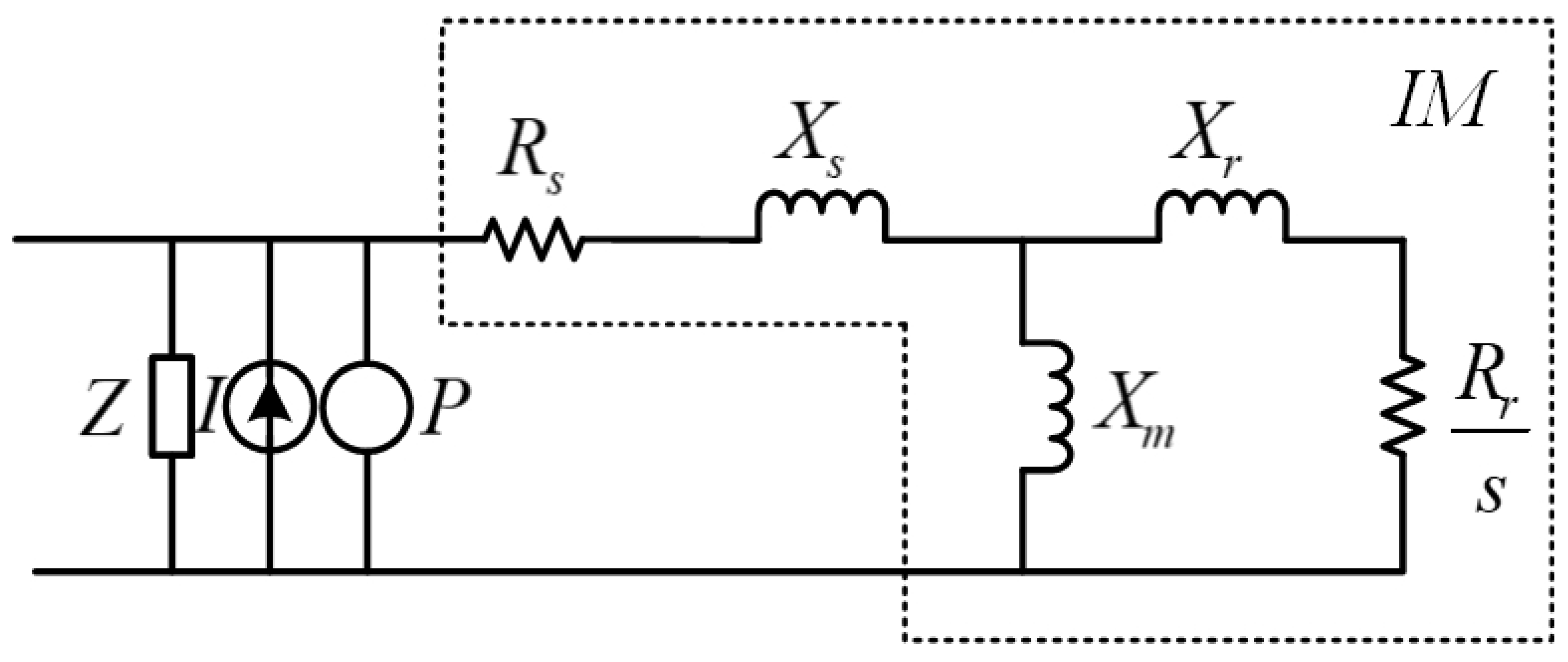
3. Induction Motor Model and Coefficient Estimation

3.1. Induction Motor Model

The dynamic part of load is usually represented by an IM model, which is discussed below [5].
d E d d t = 1 T [ E d + ( X X ) I q ] ( ω 1 ) E q d E q d t = 1 T [ E q ( X X ) I d ] + ( ω 1 ) E d d ω d t = 1 2 H [ ( A ω 2 + B ω + C ) T 0 ( E d I d + E q I q ) ] I d = 1 R s 2 + X 2 [ R s ( U d E d ) + X ( U q E q ) ] I q = 1 R s 2 + X 2 [ R s ( U q E q ) X ( U d E d ) ]
where T X r + X m R r , X X s + X m , X X s + X m X r X m + X r , A + B + C = 1 . In Equation (6), R s is motor stator winding resistance, X s is motor stator leakage reactance, X m is motor magnetizing reactance, R r is rotor resistance, X r is rotor leakage reactance, H is rotor inertia constant, ω is rotor speed, I d and I q are stator current in d-axis and q-axis, U d and U q are bus voltage in d-axis and q-axis, and E d and E q are stator voltage in d-axis and q-axis. T 0 is the initial load torque. The parameters to be identified in an IM model are: X r , X m , X s , R r , R s , A , B , C , H . Typically, A is assumed to be 1 as the mechanical torque is assumed to be proportional to the square of the rotation speed of the motor [11]. Consequently, B and C are both equal to 0.
The differential equation (Equation (7)) is non-linear and the differentiations of E d , E q , ω cannot be measured directly. These features make the procedure in ZIP models unsuitable for IM model parameter identification and complicates the estimation process. In this work, the state of IM model is assumed to follow the transitions below.
y E d [ t ] = β 1 E d [ t ] + β 2 I q [ t ] ( ω 1 ) E q [ t ] + ε E d [ t ] y E q [ t ] = β 1 E q [ t ] β 2 I d [ t ] + ( ω 1 ) E d [ t ] + ε E q [ t ] y ω [ t ] = β 3 ( ω 2 T 0 E d [ t ] I d [ t ] E q [ t ] I q [ t ] ) + ε ω [ t ] I d [ t ] = α b ( U d [ t ] E d [ t ] ) + α c ( U q [ t ] E q [ t ] ) + ε I d [ t ] I q [ t ] = α b ( U q [ t ] E q [ t ] ) α c ( U d [ t ] E d [ t ] ) + ε I q [ t ]
where y E d d E q d t , y E q d E d d t y ω d ω d t , β 1 1 T , β 2 X X T , β 3 1 2 H , α b R s R s 2 + X 2 , α c X R s 2 + X 2 , ε E d [ t ] N ( 0 , 1 / τ E ) , ε E q [ t ] N ( 0 , 1 / τ E ) , ε ω [ t ] N ( 0 , 1 / τ ω ) , ε I d [ t ] N ( 0 , 1 / τ I ) , and ε I q [ t ] N ( 0 , 1 / τ I ) .
The prior distribution of these parameters is assumed to be as follows.
β 1 N ( μ β 1 ( 0 ) , 1 / τ β 1 ( 0 ) ) , β 2 N ( μ β 2 ( 0 ) , 1 / τ β 2 ( 0 ) ) β 3 N ( μ β 3 ( 0 ) , 1 / τ β 3 ( 0 ) ) , α b N ( μ α b ( 0 ) , 1 / τ α b ( 0 ) ) α c N ( μ α c ( 0 ) , 1 / τ α c ( 0 ) ) , τ E G ( α E ( 0 ) , β E ( 0 ) ) τ ω G ( α ω ( 0 ) , β ω ( 0 ) ) , τ I G ( α I ( 0 ) , β I ( 0 ) ) .
That is, the transition of the IM model is assumed to be disturbed by some Gaussian noise and the prior distribution of the parameters follows Gaussian distributions. In this case, if the measurements of y E d , y E q , y ω , E q , E d , I d , I q , U d , U q are available, the same procedure as the one in the ZIP model section can be followed and similar posterior distribution can be obtained after some algebra. In practice, however, not all of the measurements are available. Thus, we provide a modified Gibbs sampling of the IM model.

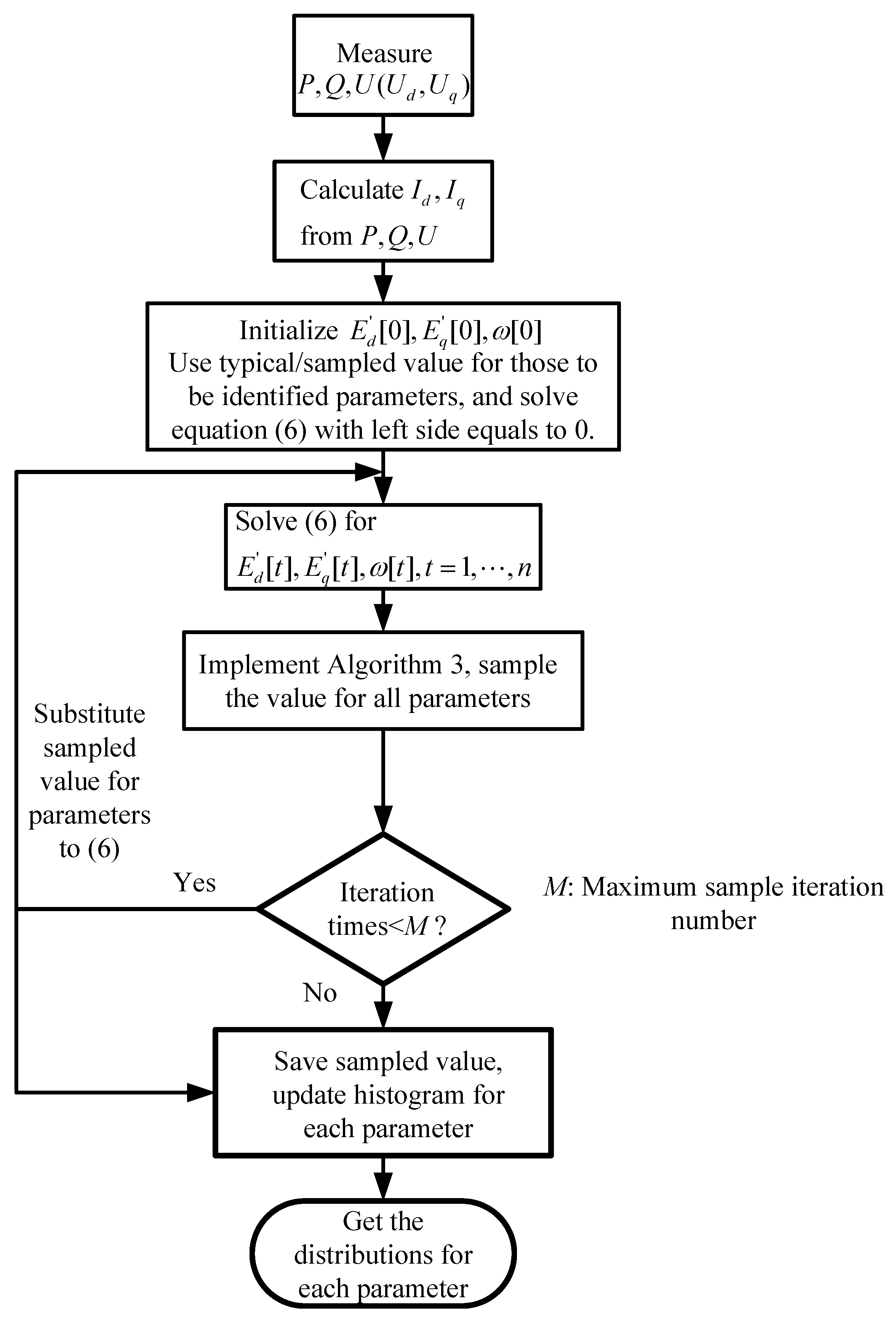
3.2. Gibbs Sampling in IM Model

If measurements of y E d , y E q , y ω , E q , E d , I d , I q , U d , U q are available, Gibbs sampling of the IM model is similar to the procedure of the ZIP model. The Gibbs sampling of the IM model can be found in Algorithm 3.
However, measurements of the derivative equations, i.e., the values of y E d , y E q , E d , E q , are not available. Thus, an iterative algorithm following the intuition of Gibbs sampling algorithm is proposed in this paper. Starting by using the typical value of corresponding parameters, Equation (6) is solved first, and a set of sampled value of y E d , y E q , E d , E q is obtained. Then, the Gibbs sampling is implemented to derive posterior distributions of the target parameters. The means of the posterior distributions are used to solve Equation (6) again and generate new samples of y E d , y E q , E d , E q . This iteration continues until the predefined maximum iteration number is reached. The flow chart of the proposed method is shown in Figure 2.
Algorithm 3 Gibbs Sampling in the ZIP model.
  • Get measurements of y E d , y E q , y ω , E q , E d , I d , I q , U d , U q .
  • Draw initial samples β 1 N ( μ β 1 ( 0 ) , 1 / τ β 1 ( 0 ) ) , β 2 N ( μ β 2 ( 0 ) , 1 / τ β 2 ( 0 ) ) , β 3 N ( μ β 3 ( 0 ) , 1 / τ β 3 ( 0 ) ) , α b N ( μ α b ( 0 ) , 1 / τ α b ( 0 ) ) , α c N ( μ α c ( 0 ) , 1 / τ α c ( 0 ) ) , τ E G ( α E ( 0 ) , β E ( 0 ) ) , τ ω G ( α ω ( 0 ) , β ω ( 0 ) ) , τ I G ( α I ( 0 ) , β I ( 0 ) ) from typical distributions.
  • For iteration k = 0 , 1 , 2 , , K
    • Draw a sample β 1 ( k + 1 ) N ( μ β 1 ( k + 1 ) , 1 / τ β 1 ( k + 1 ) ) according to Equation (A6).
    • Draw a sample β 2 ( k + 1 ) N ( μ β 2 ( k + 1 ) , 1 / τ β 2 ( k + 1 ) ) according to Equation (A7).
    • Draw a sample β 3 ( k + 1 ) N ( μ β 3 ( k + 1 ) , 1 / τ β 3 ( k + 1 ) ) according to Equation (A8).
    • Draw a sample α b k + 1 N ( μ α b ( k + 1 ) , 1 / τ α b ( k + 1 ) ) according to Equation (A9).
    • Draw a sample α c k + 1 N ( μ α c ( k + 1 ) , 1 / τ α c ( k + 1 ) ) according to Equation (A10).
    • Draw a sample τ E k + 1 G ( α E ( k + 1 ) , β E ( k + 1 ) ) according to Equation (A11).
    • Draw a sample τ ω k + 1 G ( α ω ( k + 1 ) , β ω ( k + 1 ) ) according to Equation (A12).
    • Draw a sample τ I k + 1 G ( α I ( k + 1 ) , β I ( k + ! ) ) according to Equation (A13).
    End For
  • Discard burn-in data, and the distribution estimate is the histogram samples.

4. Numerical Results

Simulation studies were carried out for ZIP and IM models, separately. In this study, the maximum Gibbs sampling runs K was set to 40,000 and the burn-in length K ̲ was chosen as 5000 [21].

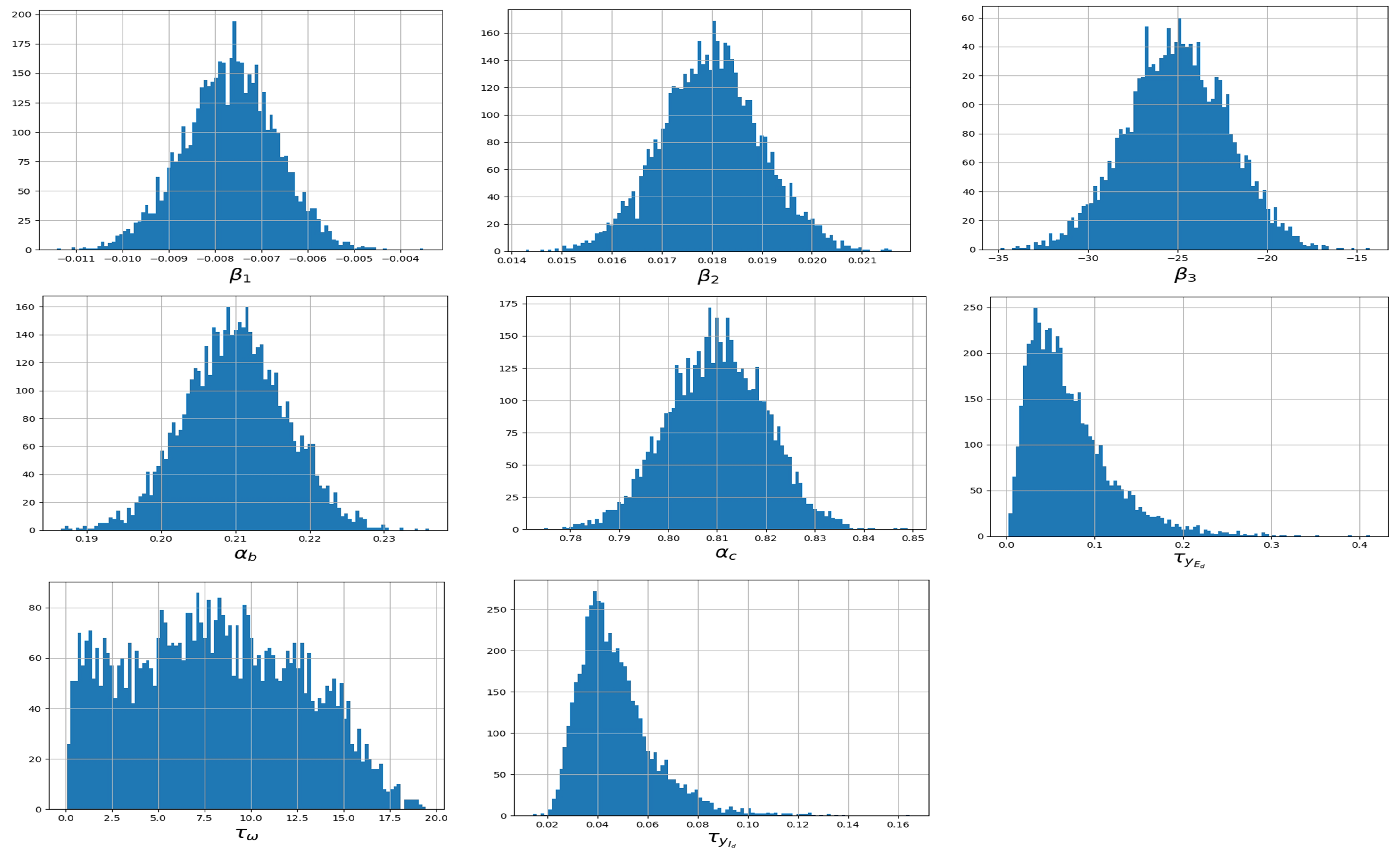
4.1. ZIP Model Identification

A 33-bus test feeder was used to generate the testing data. Load at bus 18 was replaced by a ZIP model. Randomness was added to loads at other buses by multiplying a random factor drawing from a uniform distribution following U [ 0.1 , 4.5 ] as shown in Equation (8).
P w , i = P i · U [ 0.1 , 4.5 ]
where P i is the original load in the 33-bus test feeder, i indicates the node number, and P w , i is the weighted load at the corresponding node after multiplying a random weight. The changes at each load in every experiment simulated the disturbances and uncertainties in the system, which significantly impacted the voltage and power at the bus of interest.
The ZIP factors of the load at node 18 were assigned as α 1 = 0.25 , α 2 = 0.25 , α 3 = 0.5 . Power flow converged in each iteration with different P w , i , and the corresponding voltage V w , i was recorded. The measurement noise ε followed N ( 0 , 0.1 ) , which means a 10% measurement error.
By implementing the proposed GS method, the coefficients of the ZIP model were estimated, as shown in Figure 3.
Different from other estimation approaches, the GS approach can generate a distribution that describes the probability of the real value falling into a certain range. As shown in Figure 3, the mean values of the distributions of α 1 and α 2 were found to be 0.25 and 0.249, respectively, and α 3 = 1 α 1 α 2 .
Figure 4 and Figure 5 show the voltage and voltage/real power differences, respectively, using the estimated and real model in 100 i.i.d. experiments. The randomness came from the factors multiplied to loads at other buses. The dash line in Figure 4 indicates the voltage at bus 18 using the real ZIP coefficients, and the solid line is the voltage measured at the same bus using estimated coefficients. The comparison shown in Figure 5 is the distributions of voltage and active power differences, Δ V and Δ P . It can be seen that the differences were in the range of 10−4 and 10−3 p.u., respectively. Figure 6 shows the burn-in process observed. It shows that the process was very quick, and no significant burn-in process that could be observed.

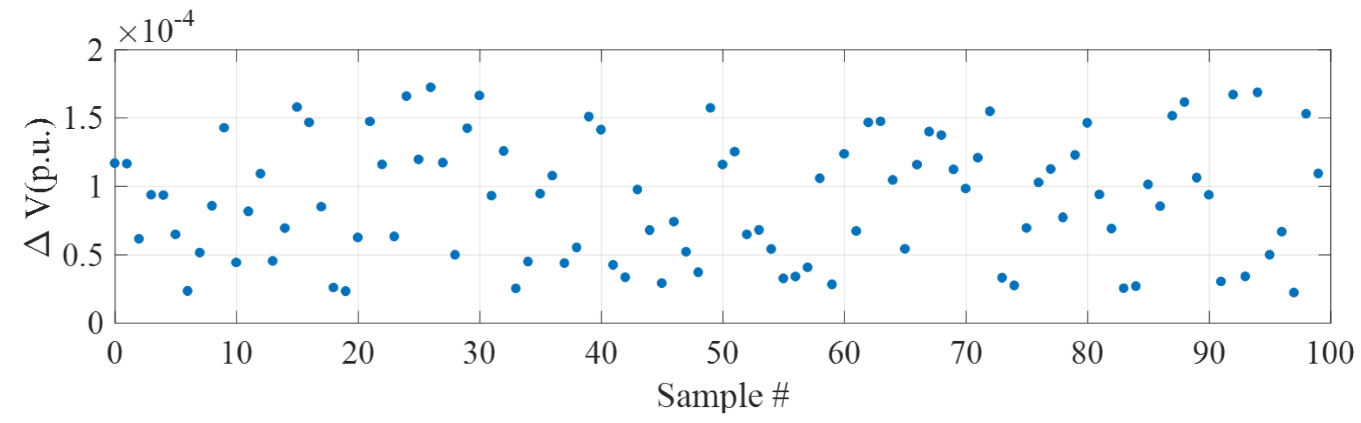
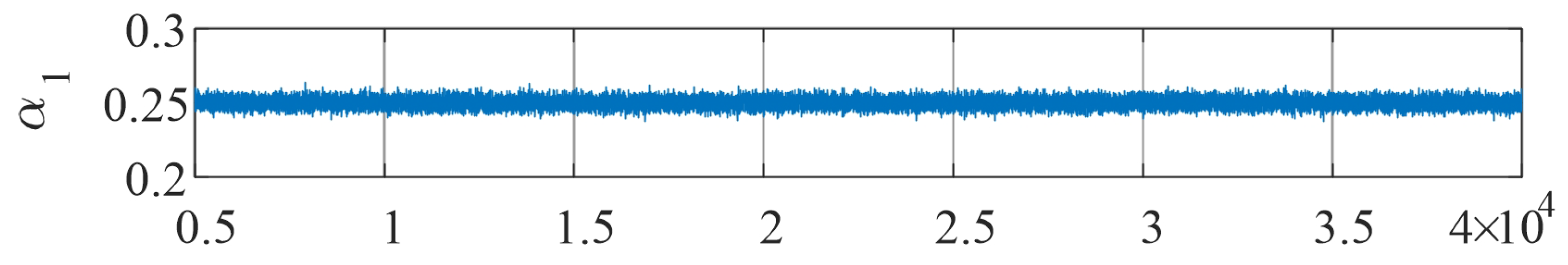
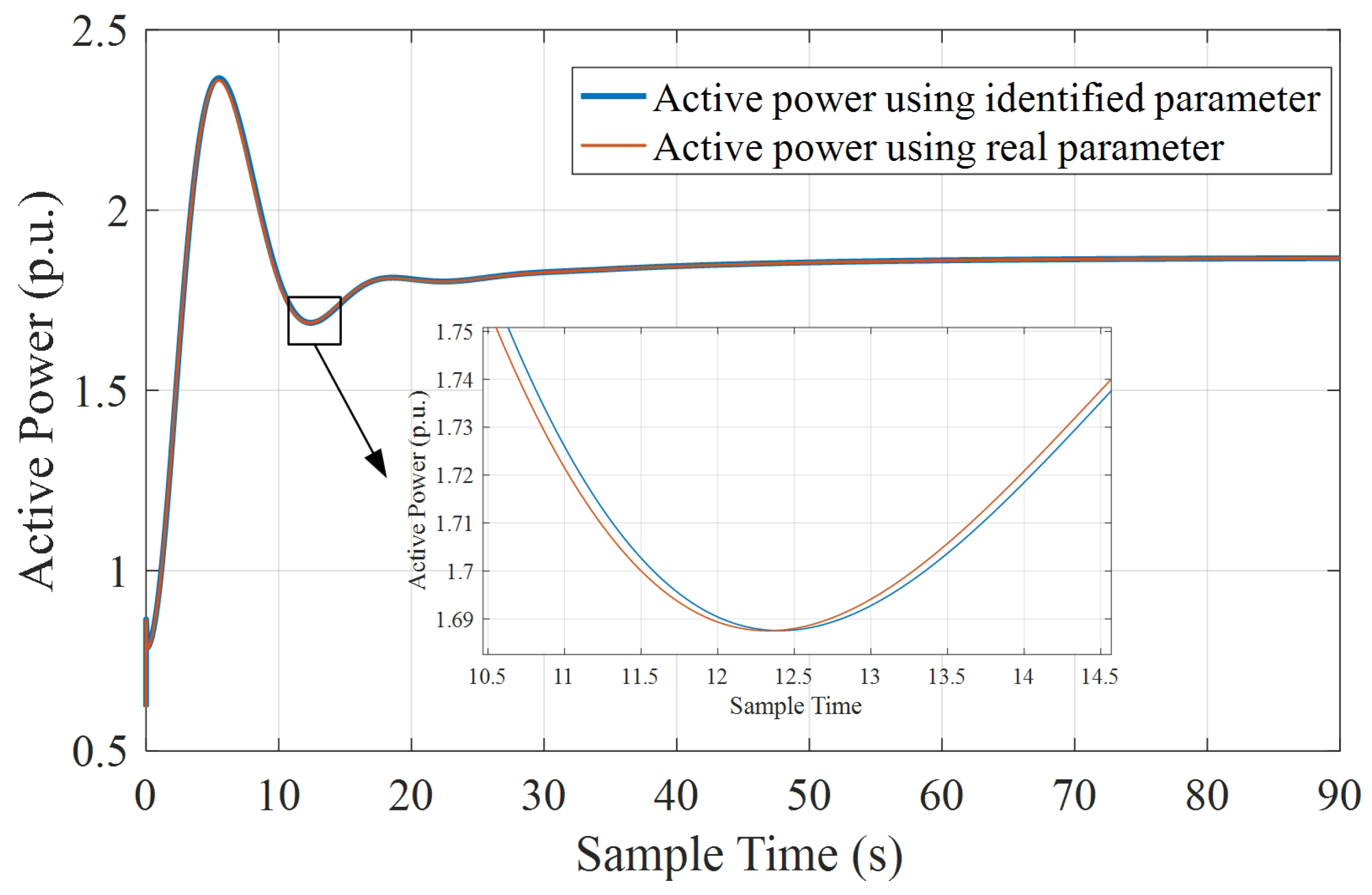
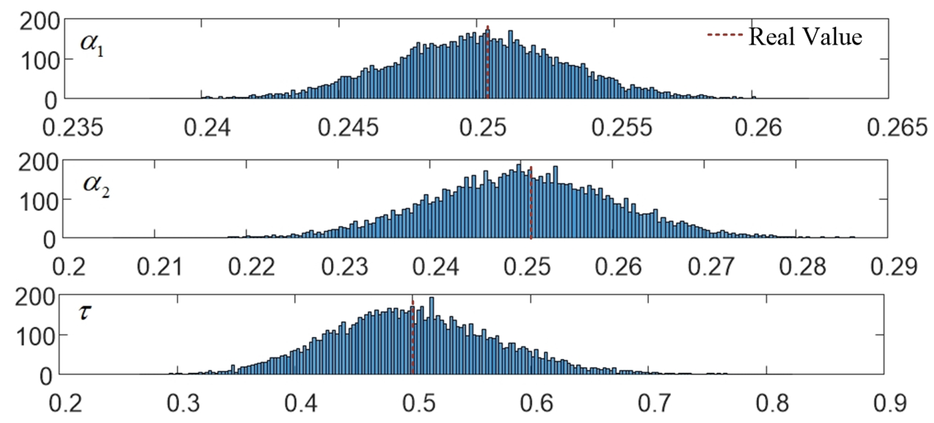
4.2. IM Model Identification
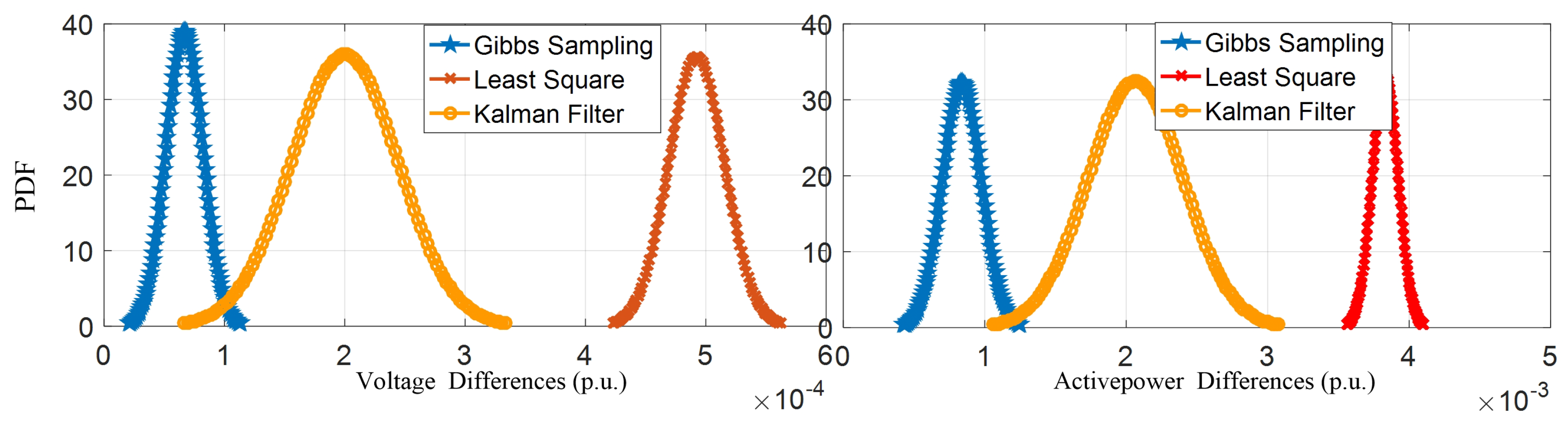
The estimation of the parameters in the IM model followed the same procedure. A dynamic model was built in Matlab/Simulink to generate the data that were used in Equation (7) in a 33 bus test feeder, as shown in Figure 7. The sampling results are shown in Figure 8 and compared with the real data in Table 1. According to Table 1, the estimation error was less than 6%, with 5% measurement error. It is worth noting that estimation of parameters highly relied on the prior distributions. A good prior could significantly increase the estimation accuracy and shorten the burn-in period. A comparison of the active power response using test parameter and identified parameteris shown in Figure 9. The simulation results also indicate the differences in active power was small and the identified parameters were accurate enough to be used in other analyses.

4.3. Benchmarks

The ZIP and IM model parameters derived by the proposed GS method were compared with least square (LS) [23] and Kalman Filter (KF) methods [24] with 10% noise. The comparison results of the voltage and active power using GS, LS, and KF in ZIP model are shown in Figure 10. The average absolute mean errors of voltage and active power in p.u. are listed in Table 2. As shown in Figure 10, it was obvious that the GS approach had the best performance, while KF method only fell slightly behind. In contrast, LS have the largest error among all three approaches when there was large measurement error. However, KF only worked well with time-invariant parameter estimation [25]. In practice, the ZIP component varies with time due to stochastic consumer behaviors.
The parameters estimation comparisons in the IM model are listed in Table 3. The estimation errors from GS were the smallest. The performance of KF was worse than itself in the ZIP model, but still better than the LS method.

5. Discussion

Some difficulties during the identification are discussed.
1
It is assumed that the noise in ZIP and IM models follows a normal distribution. In practice, the true randomness of parameters of load models is not available. By the law of large numbers, a normal distribution would be the best approximation of the randomness if the sample size is large enough. However, the robustness of the proposal needs further investigation when the Gaussian assumption is violated.
2
We are only estimating the parameters of ZIP or IM model. It is necessary to consider multiple ZIP and MI models connected to different locations in the grid. There might be inferences to the estimation.
3
How to identify a composition model composed by ZIP and IM is another interesting topic, which is a future work of this project. Most of the work that has been done in composite load modeling needs to specify the percentage of ZIP by giving the active power load P ZIP .

6. Conclusions

Bayesian estimation based dynamic load modeling is an executable and reliable composite load modeling approach. This method can overcome some disadvantages in the traditional composite load modeling process. It can provide a robust time-varying dynamic load parameter estimation with higher accuracy and better performance. It is worth noting that this method requires a good estimation of each parameter, which can be achieved by using traditional identification methods, such as Least-square, Kalman Filter, Genetic Algorithm, etc. Future work will be focused on implementing those aforementioned approaches to better estimate the prior, parameter identification in composite load model, and model clustering using machine learning approaches. Another important study is evaluating the robustness of the proposal when assumptions are violated via experiments.

Author Contributions

H.L. and Q.C. conceived of the presented idea and developed the theory. C.F. and Z.Y. performed the computations. D.S. verified the analytical methods. Z.W. encouraged C.F. and Z.Y. to investigate dynamic load modeling and supervised the findings of this work. All authors discussed the results and contributed to the final manuscript.

Funding

This work was funded by SGCC Science and Technology Program under contract no. SGSDYT00FCJS1700676.

Conflicts of Interest

The authors declare no conflict of interest. The funders had no role in the design of the study; in the collection, analyses, or interpretation of data; in the writing of the manuscript, or in the decision to publish the results.

Abbreviations

The following abbreviations are used in this manuscript:
DGsdistributed generations
IMinduction motor
ERLexponential recovery load model
LSLeast square
GAGenetic algorithm
ANNArtificial neural network
BEBayesian estimation
MLmaximum likelihood
PDFProbability density function
i.i.d.independent and identically distributed

Appendix A. Derivation of the ZIP Model

In this Appendix, we derive the posterior distribution of parameters in the ZIP model. We show that the Guassian distribution assumption makes the post distribution of these three parameters remain the same form of the priors.
In the kth iteration, samples are firstly drawn from the prior distributions
α 1 ( k ) N ( μ 1 ( k ) , 1 / τ 1 ( k ) ) , α 2 ( k ) N ( μ 2 ( k ) , 1 / τ 2 ( k ) ) , τ ( k ) G ( a ( k ) , b ( k ) ) .
and α 1 ( k ) , α 2 ( k ) , τ ( k ) are initialized. Some algebraic work yields:
p ( α 1 | α 2 ( k ) , τ ( k ) , x , y ) p ( x , y | α 1 , α 2 ( k ) , τ ( k ) ) p ( α 1 )
where p ( α 1 | α 2 ( k ) , τ ( k ) , x , y ) is the posterior probability given the samples of x , y , α 2 , and τ , p ( x , y | α 1 , α 2 ( k ) , τ ( k ) ) is the likelihood in Equation (2), and p ( α 1 ) is the prior estimation following Equation (3). Taking the log form on both sides of Equation (A1) yields
log p ( α 1 | α 2 ( k ) , τ ( k ) , x , y ) τ 1 ( k ) 2 ( α 1 μ 1 ( k ) ) 2 τ ( k ) 2 t = 1 n y [ t ] ( α 1 x [ t ] 2 + α 2 ( k ) x [ t ] + 1 α 1 α 2 ( k ) ) 2
Taking log form helps convert the multiplications of the probabilities to summations, which can significantly simplify calculations when updating the distributions of the posteriors. For a normal distribution y N ( μ , 1 / τ ) , the log dependence on y is τ 2 ( y μ ) 2 τ 2 y 2 + τ μ y .
The right hand side of Equation (A2) can be further written as the following if the terms not related to α 1 are omitted.
τ 1 ( k ) + τ ( k ) t = 1 n ( x [ t ] 2 1 ) 2 α 1 2 / 2 + τ 1 ( k ) μ 1 ( k ) τ ( k ) t = 1 n ( α 2 ( k ) 1 α 2 ( k ) x [ t ] + y [ t ] ) ( 1 x [ t ] 2 ) α 1
Defining
μ 1 ( k + 1 ) τ 1 ( k ) μ 1 ( k ) τ ( k ) t = 1 n ( α 2 ( k ) 1 α 2 ( k ) x [ t ] + y [ t ] ) ( 1 x [ t ] 2 ) τ 1 ( k ) + τ ( k ) t = 1 n ( x [ t ] 2 1 ) 2 , τ 1 ( k + 1 ) τ 1 ( k ) + τ ( k ) t = 1 n ( x [ t ] 2 1 ) 2 ,
yields
α 1 | α 2 ( k ) , τ ( k ) , τ 1 ( k ) , μ 1 ( k ) , x , y N ( μ 1 ( k + 1 ) , 1 / τ 1 ( k + 1 ) ) .
A new α 1 is sampled from the estimated distribution N ( μ 1 ( k + 1 ) , τ 1 ( k + 1 ) ) as α 1 ( k + 1 ) . Following a similar procedure, α 2 can be derived. Define
μ 2 ( k + 1 ) τ 2 ( k ) μ 2 ( k ) τ ( k ) t = 1 n ( α 1 ( k + 1 ) 1 α 1 ( k + 1 ) x [ t ] + y [ t ] ) ( 1 x [ t ] ) τ 2 ( k ) + τ ( k ) t = 1 n ( x [ t ] 1 ) 2 , τ 2 ( k + 1 ) τ 2 ( k ) + τ ( k ) i = 1 n ( x [ t ] 1 ) 2 .
Therefore, the following can be derived:
α 2 | α 1 ( k + 1 ) , τ ( k ) , τ 1 ( k ) , μ 1 ( k ) , x , y N ( μ 2 ( k + 1 ) , 1 / τ 2 ( k + 1 ) ) .
For τ , the posterior given by new samples of α 1 ( k + 1 ) and α 2 ( k + 1 ) can be written as p ( τ | α 1 ( k + 1 ) , α 2 ( k + 1 ) , x , y ) p ( x , y | α 1 ( k + 1 ) , α 2 ( k + 1 ) , τ ) p ( τ ) . Taking the log form of both sides of the posterior yields
log p ( τ | α 1 ( k + 1 ) , α 2 ( k + 1 ) , x , y ) n 2 log τ τ 2 t = 1 n y [ t ] α 1 ( k + 1 ) x [ t ] 2 α 2 ( k + 1 ) x [ t ] 1 + α 1 ( k + 1 ) + α 2 ( k + 1 ) + ( a ( k ) 1 ) log τ b ( k ) τ .
Define
a ( k + 1 ) = a ( k ) + n / 2 , b ( k + 1 ) = b ( k ) + t = 1 n y [ t ] α 1 ( k + 1 ) x [ t ] 2 α 2 ( k + 1 ) x [ t ] ( 1 α 1 ( k + 1 ) α 2 ( k + 1 ) ) 2 / 2 .
the posterior τ | α 1 ( k + 1 ) , α 2 ( k + 1 ) , x , y G ( a ( k + 1 ) , b ( k + 1 ) ) can be obtained.

Appendix B. Derivation of the IM Model

If measurements of y E d , y E q , y ω , E q , E d , I d , I q , U d , U q are available, Gibbs sampling of the IM model is similar to the procedure of the ZIP model. The detailed algebra is omitted here for space considerations. The post distributions of parameters remain the same form of the one of the priors.
Define
μ β 1 ( k + 1 ) = τ β 1 ( k ) μ β 1 ( k ) + τ E ( k ) t = 1 n E d [ t ] y E d [ t ] + E q [ t ] y E q [ t ] β 2 ( k ) ( E d [ t ] I q [ t ] E q [ t ] I d [ t ] ) τ β 1 ( k ) + τ E ( k ) t = 1 n ( E d [ t ] 2 + E q [ t ] 2 ) , τ β 1 ( k + 1 ) = 1 τ β 1 ( k ) + τ E ( k ) t = 1 n ( E d [ t ] 2 + E q [ t ] 2 )
the posterior β 1 | β 2 ( k ) , y E d , y E q , y ω , E q , E d , I d , I q , U d , U q , τ E ( k ) , τ β 1 ( k ) , μ β 1 ( k ) N ( μ β 1 ( k + 1 ) , τ β 1 ( k + 1 ) ) can be obtained.
Define
μ β 2 ( k + 1 ) = τ β 2 ( k ) μ β 2 ( k ) + τ E ( k ) t = 1 n y E d [ t ] I q [ t ] y E q [ t ] I d [ t ] + β 1 ( k + 1 ) ( E d [ t ] I q [ t ] E q [ t ] I d [ t ] ) + ( ω [ t ] 1 ) ( E d [ t ] I d [ t ] + E q [ t ] I q [ t ] ) τ β 2 ( k ) + τ E ( k ) t = 1 n ( I d [ t ] 2 + I q [ t ] 2 ) , τ β 2 ( k + 1 ) = 1 τ β 2 ( k ) + τ E ( k ) i = 1 n ( I d [ t ] 2 + I q [ t ] 2 ) .
the posterior β 2 | β 1 ( k + 1 ) , y E d , y E q , y ω , E q , E d , I d , I q , U d , U q , τ E ( k ) , τ β 2 ( k ) , μ β 2 ( k ) N ( μ β 2 ( k + 1 ) , τ β 2 ( k + 1 ) ) can be obtained.
Define
μ β 3 ( k + 1 ) = τ β 3 ( k ) μ β 3 ( k ) τ ω ( k ) t = 1 n y ω [ t ] ( ω [ t ] 2 T 0 + E d [ t ] I d [ t ] + E q [ t ] I q [ t ] ) τ β 3 ( k ) + τ ω ( k ) t = 1 n ω [ t ] 4 T 0 2 + ( E d [ t ] I d [ t ] + E q [ t ] I q [ t ] ) 2 2 ω [ t ] 2 T 0 ( E d [ t ] I d [ t ] + E q [ t ] I q [ t ] ) , τ β 3 ( k + 1 ) = 1 τ β 3 ( k ) + τ ω ( k ) t = 1 n ω [ t ] 4 T 0 2 + ( E d [ t ] I d [ t ] + E q [ t ] I q [ t ] ) 2 2 ω [ t ] 2 T 0 ( E d [ t ] I d [ t ] + E q [ t ] I q [ t ] ) .
the posterior β 3 | y E d , y E q , y ω , E q , E d , I d , I q , U d , U q , τ E ( k ) , τ β 3 ( k ) , μ β 3 ( k ) N ( μ β 3 ( k + 1 ) , τ β 3 ( k + 1 ) ) can be obtained.
Define
μ α b ( k + 1 ) = τ α b ( k ) μ α b ( k ) + τ I ( k ) t = 1 n I d [ t ] ( U d [ t ] E d [ t ] ) + I q [ t ] ( U q [ t ] E q [ t ] ) τ α b ( k ) + τ I ( k ) t = 1 n ( U d [ t ] E d [ t ] ) 2 + ( U q [ t ] E q [ t ] ) 2 , τ α b ( k + 1 ) = 1 τ α b ( k ) + τ I ( k ) t = 1 n ( U d [ t ] E d [ t ] ) 2 + ( U q [ t ] E q [ t ] ) 2
the posterior α b | y E d , y E q , y ω , E q , E d , I d , I q , U d , U q , τ I ( k ) , τ α b ( k ) , μ α b ( k ) N ( μ α b ( k + 1 ) , τ α b ( k + 1 ) ) can be obtained.
Define
μ α c ( k + 1 ) = τ α c ( k ) μ α c ( k ) + τ I ( k ) t = 1 n I d [ t ] ( U d [ t ] E d [ t ] ) I q [ t ] ( U q [ t ] E q [ t ] ) τ α c ( k ) + τ I ( k ) t = 1 n ( U d [ t ] E d [ t ] ) 2 + ( U q [ t ] E q [ t ] ) 2 , τ α c ( k + 1 ) = 1 τ α c ( k ) + τ I ( k ) t = 1 n ( U d [ t ] E d [ t ] ) 2 + ( U q [ t ] E q [ t ] ) 2
the posterior α c | y E d , y E q , y ω , E q , E d , I d , I q , U d , U q , τ I ( k ) , τ α c ( k ) , μ α c ( k ) N ( μ α c ( k + 1 ) , τ α c ( k + 1 ) ) can be obtained.
Other parameters can be obtained as follows:
τ E ( k + 1 ) | y E d , y E q , y ω , E q , E d , I d , I q , U d , U q , β 1 ( k + 1 ) , β 2 ( k + 1 ) G ( α E ( k + 1 ) , β E ( k + 1 ) )
where
α E ( k + 1 ) = α E ( k ) + n / 2 , β E ( k + 1 ) = β E ( k ) + t = 1 n y E d [ t ] β 1 ( k + 1 ) E q [ t ] β 2 ( k + 1 ) I d [ t ] + ( ω [ t ] 1 ) E q [ t ] 2 + [ y E q [ t ] β 1 ( k + 1 ) E d [ t ] + β 2 ( k + 1 ) I q [ t ] ( ω [ t ] 1 ) E d [ t ] 2 2 .
τ ω ( k + 1 ) | y E d , y E q , y ω , E q , E d , I d , I q , U d , U q , β 3 ( k + 1 ) G ( α ω ( k + 1 ) , β ω ( k + 1 ) )
where
α ω ( k + 1 ) = α ω ( k ) + n / 2 , β ω ( k + 1 ) = β ω ( k ) + 1 2 t = 1 n y ω [ t ] β 3 ( k + 1 ) ( ω [ t ] 2 T 0 E d [ t ] I d [ t ] E q [ t ] I q [ t ] ) 2
τ I ( k + 1 ) | y E d , y E q , y ω , E q , E d , I d , I q , U d , U q , α b ( k + 1 ) , α c ( k + 1 ) G ( α I ( k + 1 ) , β I ( k + 1 ) )
where
α I ( k + 1 ) = α I ( k ) + n / 2 , β I ( k + 1 ) = β I ( k ) + t = 1 n I d [ t ] α b ( k + 1 ) ( U d [ t ] E d [ t ] ) α c ( k + 1 ) ( U q [ t ] E q [ t ] ) 2 + I q [ t ] α b ( k + 1 ) ( U q [ t ] E q [ t ] ) + α c ( k + 1 ) ( U d [ t ] E d [ t ] ) 2 2 .

References

  1. Arif, A.; Wang, Z.; Wang, J.; Mather, B.; Bashualdo, H.; Zhao, D. Load Modeling—A Review. IEEE Trans. Smart Grid 2017. [Google Scholar] [CrossRef]
  2. Milanovic, J.V.; Yamashita, K.; Martínez Villanueva, S.; Djokic, S.Ž.; Korunović, L.M. International Industry Practice on Power System Load Modeling. IEEE Trans. Power Syst. 2013, 8, 3038–3046. [Google Scholar] [CrossRef]
  3. Milanović, J.V.; Mat Zali, S. Validation of Equivalent Dynamic Model of Active Distribution Network Cell. IEEE Trans. Power Syst. 2013, 8, 2101–2110. [Google Scholar] [CrossRef]
  4. Bokhari, A.; Alkan, A.; Dogan, R.; Diaz-Aguiló, M.; León, F.D.; Czarkowski, D.; Zabar, Z.; Birenbaum, L.; Noel, A.; Uosef, R.E. Experimental Determination of the ZIP Coefficients for Modern Residential, Commercial, and Industrial Loads. IEEE Trans. Power Deliv. 2014, 1372–1381. [Google Scholar] [CrossRef]
  5. Renmu, H.; Jin, M.; Hill, D.J. Composite Load Modeling Via Measurement Approach. IEEE Trans. Power Syst. 2006, 5, 663–672. [Google Scholar] [CrossRef]
  6. Tang, Y.; Zhao, S.; Ten, C.-W.; Zhang, K. Enhancement of Distribution Load Modeling Using Statistical Hybrid Regression. In Proceedings of the Power & Energy Society Innovative Smart Grid Technologies Conference (ISGT), Washington, DC, USA, 23–26 April 2017; pp. 1–5. [Google Scholar]
  7. Alyami, S.; Wang, C.; Fu, C. Development of Autonomous Schedules of Controllable Loads for Cost Reduction and PV Accommodation in Residential Distribution Networks. In Proceedings of the Electrical Power and Energy Conference (EPEC), London, ON, Canada, 26–28 October 2015; pp. 81–86. [Google Scholar]
  8. Ten, C.-W.; Tang, Y. Electric Power: Distribution Emergency Operation; CRC Press: Boca Raton, FL, USA, 2018. [Google Scholar]
  9. Kundur, P.; Balu, N.; Lauby, M. Power System Stability and Control; McGraw-Hill: New York, NY, USA, 1994. [Google Scholar]
  10. Fu, C.; Wang, C.; Alyami, S. An LMI Based Stability Margin Analysis for Active PV Power Control of Distribution Networks with Time-Invariant Delays. arXiv, 2018; arXiv:1804.06903. [Google Scholar]
  11. Kim, J.-K.; An, K.; Ma, J.; Shin, J.; Song, K.-B.; Park, J.-D.; Park, J.-W.; Hur, K. Fast and Reliable Estimation of Composite Load Model Parameters Using Analytical Similarity of Parameter Sensitivity. IEEE Trans. Power Syst. 2016, 1, 663–671. [Google Scholar] [CrossRef]
  12. Singh, D.; Misra, R.K. Effect of Load Models in Distributed Generation Planning. IEEE Trans. Power Syst. 2007, 11, 2204–2212. [Google Scholar] [CrossRef]
  13. Al Abri, R.S.; El-Saadany, E.F.; Atwa, Y.M. Optimal Placement and Sizing Method to Improve the Voltage Stability Margin in a Distribution System using Distributed Generation. IEEE Trans. Power Syst. 2013, 2, 326–334. [Google Scholar] [CrossRef]
  14. Ge, Y.; Flueck, A.J.; Kim, D. K.; Ahn, J.B.; Lee, J.D.; Kwon, D.Y. An Event-Oriented Method for Online Load Modeling Based on Synchrophasor Data. IEEE Trans. Smart Grid 2015, 7, 2060–2068. [Google Scholar] [CrossRef]
  15. Vignesh, V.; Chakrabarti, S.; Srivastava, S.C. Classification and Modelling of Loads in Power Systems using SVM and Optimization Approach. In Proceedings of the Power & Energy Society General Meeting, Denver, CO, USA, 26–30 July 2015; pp. 1–5. [Google Scholar]
  16. Patel, A.; Wedeward, K.; Smith, M. Parameter Estimation for Inventory of Load Models in Electric Power Systems. In Proceedings of the World Congress on Engineering and Computer Science, San Francisco, CA, USA, 22–24 October 2014; pp. 22–24. [Google Scholar]
  17. Bao, Y.; Wang, L.; Wang, C.; Wang, Y. Hammerstein Models and Real-Time System Identification of Load Dynamics for Voltage Management. IEEE Access 2018, 2060–2068. [Google Scholar] [CrossRef]
  18. Chang, G.W.; Chen, C.I.; Liu, Y.J. A Neural-Network-Based Method of Modeling Electric Arc Furnace Load for Power Engineering Study. IEEE Trans. Power Syst. 2010, 2, 138–146. [Google Scholar] [CrossRef]
  19. Wang, C.; Wang, Z.; Wang, J.; Zhao, D. Robust Time-Varying Parameter Identification for Composite Load Modeling. IEEE Trans. Smart Grid 2017, 1949–3053. [Google Scholar] [CrossRef]
  20. Zhao, J.; Wang, Z.; Wang, J. Robust Time-Varying Load Modeling for Conservation Voltage Reduction Assessment. IEEE Trans. Smart Grid 2018, 7, 3304–3312. [Google Scholar] [CrossRef]
  21. Meyn, S.P.; Tweedie, R.L. Markov Chains and Stochastic Stability; Springer Science & Business Media: London, UK, 2012. [Google Scholar]
  22. Lynch, S. Introduction to Applied Bayesian Statistics and Estimation for Social Scientists; Springer Science & Business Media: New York, NY, USA, 2007. [Google Scholar]
  23. Liu, Q.; Chen, Y.; Duan, D. The Load Modeling and Parameters Identification for Voltage Stability Analysis. In Proceedings of the International Conference on Power System Technology, Kunming, China, 13–17 October 2002; pp. 2030–2033. [Google Scholar]
  24. Lee, S.-H.; Son, S.-E.; Lee, S.-M.; Cho, J.-M.; Song, K.-B.; Park, J.-W. Kalman-Filter Based Static Load Modeling of Real Power System using K-EMS Data. J. Electr. Eng. Technol. 2012, 7, 304–311. [Google Scholar] [CrossRef]
  25. Best, M.C.; Gordon, T.J.; Dixon, P.J. An Extended Adaptive Kalman Filter for Real-time State Estimation of Vehicle Handling Dynamics. Veh. Syst. Dyn. 2000, 34, 57–75. [Google Scholar] [Green Version]
Figure 1. The composite model of ZIP + IM.
Energies 12 00547 g001
Figure 2. Flow chart of Gibbs sampling in IM model.
Energies 12 00547 g002
Figure 3. The estimated parameters of the ZIP model.
Energies 12 00547 g003
Figure 4. Voltage comparison at bus 18 between the simulations using the real parameter and estimated parameter.
Energies 12 00547 g004
Figure 5. Comparison of the absolute values of Δ V and Δ P between connecting real ZIP model and the estimated ZIP model at bus 18.
Energies 12 00547 g005
Figure 6. The burn-in process of sampling α 1 .
Energies 12 00547 g006
Figure 7. The topology of the 33 bus system with IM.
Energies 12 00547 g007
Figure 8. The estimated parameter distributions of the IM model.
Energies 12 00547 g008
Figure 9. Comparison of the active power between simulations using test parameter and identified parameter.
Energies 12 00547 g009
Figure 10. The absolute error distributions of voltage and active power using GS, LS and KF, respectively.
Energies 12 00547 g010
Table 1. Estimated and real value of the parameters for IM mode with 5% measurement error.
Para.Real ValueEst. Value (Mean)Error (%)
β 1 0.00770.0076830.22
β 2 0.0180.018241.33
β 3 2524.80.8
α b 0.200.2115.5
α c 0.800.8131.63
Table 2. Active power and voltage errors with different methods.
Para. ErrorGS (%)LS (%)KF (%)
Voltage0.0070.0620.024
Active Power1.124.652.64
Table 3. IM model parameter estimation with different methods.
Para.GSLSKFReal Value
β 1 0.0076830.00760.00770.0077
β 2 0.018240.13750.01850.018
β 3 24.8183425
α b 0.2112.061.80.2
α c 0.8134.0430.8

