Effects of Producer and Transmission Reliability on the Sustainability Assessment of Power System Networks

Abstract

Details are presented of the development and incorporation of a generation and transmission reliability approach in an upper-level sustainability assessment framework for power system planning. This application represents a quasi-stationary, multiobjective optimization problem with nonlinear constraints, load uncertainties, stochastic effects for renewable energy producers, and the propagation of uncertainties along the transmission lines. The Expected Energy Not Supplied (EENS) accounts for generation and transmission reliability and is based on a probabilistic as opposed to deterministic approach. The optimization is developed for three scenarios. The first excludes uncertainties in the load demand, while the second includes them. The third scenario accounts not only for these uncertainties, but also for the stochastic effects related to wind and photovoltaic producers. The sustainability-reliability approach is applied to the standard IEEE Reliability Test System. Results show that using a Mixture of Normals Approximation (MONA) for the EENS formulation makes the reliability analysis simpler, as well as possible within a large-scale optimization. In addition, results show that the inclusion of renewable energy producers has some positive impact on the optimal synthesis/design of power networks under sustainability considerations. Also shown is the negative impact of renewable energy producers on the reliability of the power network.

1. Introduction

Power network sustainability-reliability is an important aspect of an energy generation-transmission system because the electricity demand of a group of customers needs to be assured at every instant of time with the lowest possible price and the least damage to the environment and society [1,2,3,4]. The reliability of a power network is usually dependent on the uncertainties associated with generation [5,6,7,8,9], transmission (and distribution) [10,11,12], load demand [13,14,15], and the presence of unexpected catastrophic events [16,17,18]. On the other hand, the sustainability of a power network depends on four pillars, i.e., economic, technical, environmental, and societal [19,20]. These two main characteristics, i.e., sustainability and reliability, make the planning and design/operation optimization of a power network a difficult problem to solve [21,22]. Several methodologies have been developed independently to find solutions for these problems [23,24,25]. However, new methodologies that capture all of the aspects of sustainability and reliability and their integration into a single framework are necessary for a more detailed understanding of the planning and operational optimization and performance analysis of power networks.

In [26], the reliability of a power network is studied when decentralized generators are added to the system. A result of this study is that because of the weather dependency of some renewable energy technologies, adding a high number of renewables may cause instabilities in the network. In [27], the reliability of the power network is also studied when renewable energy technologies are added to an existing network. The part-load performance (start and ramp rates) of the thermal plants is significantly degraded in the location where renewable energy technologies are added. In [16], a reliability and evaluation assessment of a transmission grid subject to cascading failures is presented. It focuses on the impact of extreme weather on the reliability of the network. The catastrophic events are taken into account via a stochastic model based on the annual history of weather conditions in the area under study. In [28], a methodology is proposed for quantifying the transmission reliability margin when uncertainties in the network are present due to a transfer of power. A bootstrap technique is used to generate different scenarios and to quantify the transmission reliability margin with good accuracy. In [29], a methodology is proposed for the reliability evaluation of radial distribution networks. The methodology is based on an AC multiobjective optimization of repair times, failure rates, costs, and reliability.

Bi-level models are also used for power network planning under sustainability/reliability considerations with the aim of obtaining a more detailed description of the generation/transmission infrastructure, the individual technologies, and their interactions. This type of approach results in a detailed study at two different hierarchical levels, where each level with a single objective function or multiple ones depends on a different set of independent decision variables.

In [30], a bi-level programming approach to study the vulnerability of a power network is used. The upper level analyzes the effect of outages on the network, while the lower level analyzes the effect of these outages on the system operator. In the bi-level approach of [31], the upper level optimizes the dispatch of distributed generation and the cost of market purchases, while the lower level maximizes social welfare. In [32], the upper level selects the location and contract pricing of distributed generation, while the lower level measures the reaction of the distribution company. In [33], a methodology for microgrid power and reserve capacity planning is proposed with the goal to reduce microgrid capital and operational costs and assure a reliable supply of energy to the customers. The upper level optimizes the microgrid configurations, and the lower level optimizes the reserve capacity, which directly affects the reliability of the distribution system operator. In [21], a bi-level sustainability-reliability assessment framework for power networks and their interaction with microgrids is proposed. The upper level develops the synthesis/design/operation optimization of the producers and transmission lines, while the lower level takes care of the synthesis/design/operation optimization of the producers targeted by the upper level to be part of the power network configuration.

In this paper, a probabilistic generation-transmission reliability approach is proposed to be used in the upper-level Sustainability Assessment Framework (SAF) of [21]. The reliability approach takes into account, at every node and instant of time, the propagation of uncertainties along the transmission lines, the uncertainties of the generation system (including the fluctuating effects associated with the wind and photovoltaic energy producers), and the uncertainties of the load demand. This generation-transmission reliability approach is also capable of incorporating in a straightforward manner methodologies such as that of [16] to account for the contribution of unexpected catastrophic events to the reliability of a power network.

The remainder of the paper is organized as follows. Section 2 describes the system under study, while Section 3 outlines the SAF and the generation-transmission reliability approach. Section 4 then provides a description of the different scenarios considered for the analysis followed by Section 5, which presents the results of the application of the SAF to the system under study. The paper concludes with a set of conclusions in Section 6.

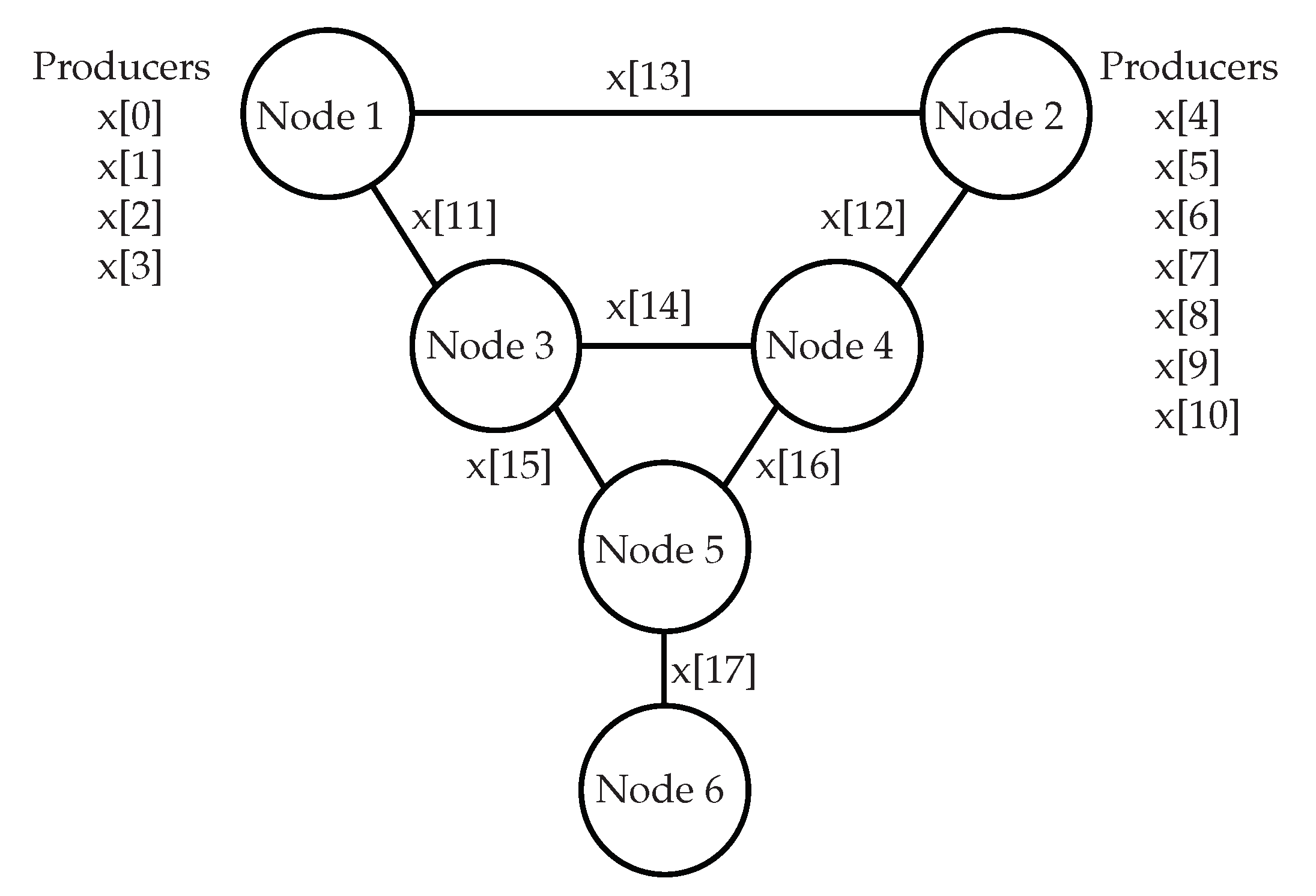
2. Description of the System

The IEEE Reliability Test System (RTS) [34] is used as a study case to evaluate the methodology proposed in this work. The single-line diagram of the RTS is shown in Figure 1. The system is composed of 11 generation units and seven transmission lines, as well as one node where only generation capacity is present (Node 1), four nodes where only load demand is present (Nodes 3 to 6), and one node where generation capacity and load demand are present (Node 2). The original RTS model considers two transmission lines between Nodes 1 and 3 and two between Nodes 2 and 4. In this work, a single line with the capacity of the two lines added together is considered instead for each set of nodes.

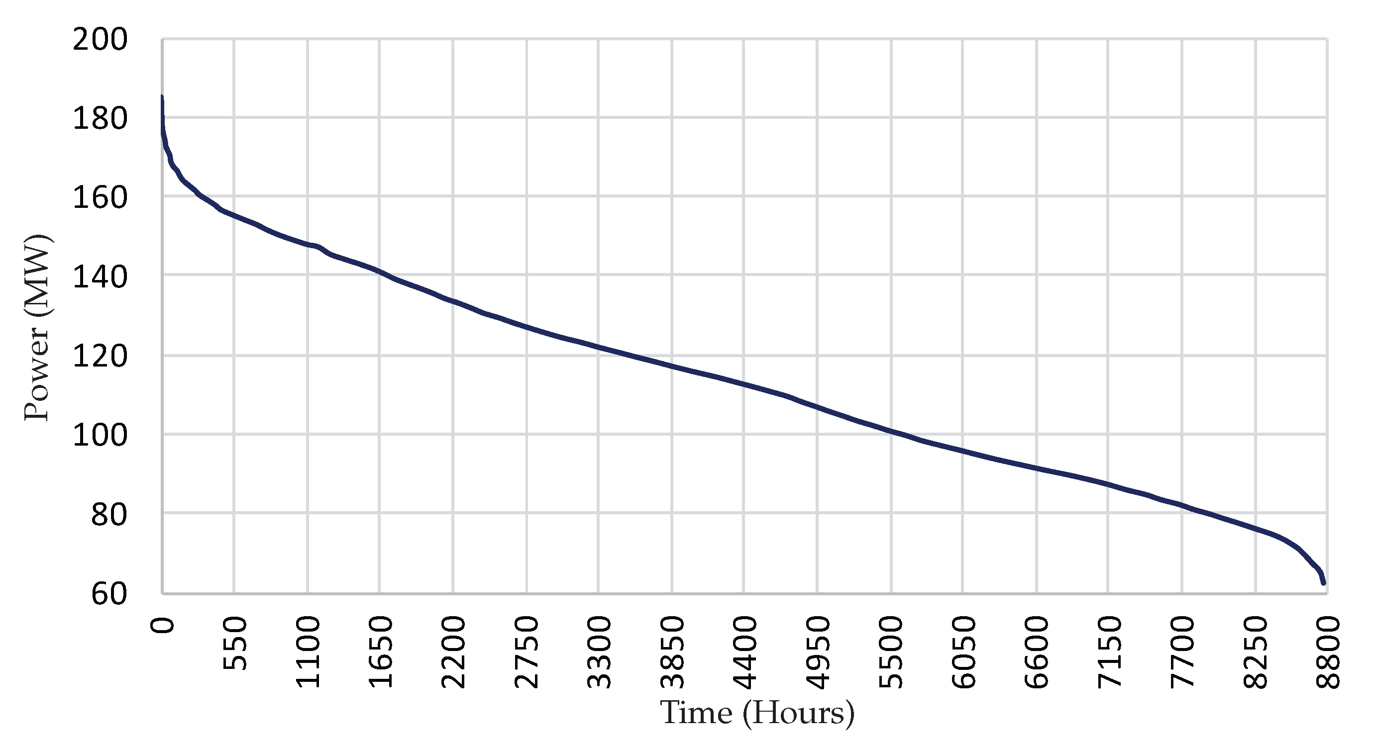
The annual peak load for the RTS is 185 MW [35]. A Load Duration Curve (LDC) is constructed for the model based on [34,35] and is shown in Figure 2. The load in each node is a fixed percentage of the load in the RTS as given in

Table 1. Load demand and installed capacity in the nodes of the RTS [34].

Node	% of the Total Load	Installed Capacity (MW)
1	0	110
2	10.81	130
3	45.95	0
4	21.62	0
5	10.81	0
6	10.81	0

. The installed capacity in each node is also given in Table 1. Five different types of producers are considered for the analysis, i.e., hydro, Ultra Supercritical Coal (USC), Natural Gas Combined Cycle (NGCC), Combustion Turbine (CT), and Reciprocating Internal Combustion Engine (RICE). The producer characteristics for the RTS are given in

Table 2. Characteristics of the producers [34,36].

Decision Variable	Type of Producer	${\mathit{P}}_{\mathit{i},\mathit{n}}^{\mathrm{Cap}}$ (MW)	${\mathit{M}}_{\mathit{i},\mathit{n},\$}^{\mathrm{Cap}}$ ($/MW-day)	${\mathit{M}}_{\mathit{i},\mathit{n},\$}^{O\&M}$ ($/MW-day)	${\mathit{\gamma }}_{\mathit{i},\mathit{n},\$}$ ($/MW)	FOR${}_{\mathit{i},\mathit{n}}$
x[0]	USC	40	799.35	115.34	4.60	0.030
x[1]	NGCC	40	215.01	30.14	3.50	0.030
x[2]	CT	10	242.05	47.95	3.50	0.020
x[3]	RICE	20	295.03	18.90	5.85	0.025
x[4]	Hydro	5	645.46	38.71	0.00	0.010
x[5]	Hydro	5	645.46	38.71	0.00	0.010
x[6]	Hydro	40	645.46	38.71	0.00	0.020
x[7]	Hydro	20	645.46	38.71	0.00	0.015
x[8]	Hydro	20	645.46	38.71	0.00	0.015
x[9]	Hydro	20	645.46	38.71	0.00	0.015
x[10]	Hydro	20	645.46	38.71	0.00	0.015

. The six nodes of the RTS are connected by seven transmission lines with a transmission voltage level of 230 kV [34]. The capacity of each of the transmission lines is given in

Table 3. Characteristics of the transmission lines [34,37].

Decision Variable	${\mathit{L}}_{\mathit{n},\mathit{m}}$ (km)	${\mathit{P}}_{\mathit{n},\mathit{m}}^{\max }$ (MW)	${\mathit{X}}_{\mathit{n},\mathit{m}}$ ($\Omega$)	${\mathit{\gamma }}_{\mathit{n},\mathit{m},\$}$ ($/MW-day)
x[11]	300	196	380.88	112.12
x[12]	1000	196	1269.6	373.73
x[13]	200	98	253.92	74.75
x[14]	50	98	63.48	18.69
x[15]	50	98	63.48	18.69
x[16]	50	98	63.48	18.69
x[17]	50	98	63.48	18.69

.

3. Sustainability Assessment Approach

The upper-level SAF developed by Cano-Andrade et al. [21] is used here to optimize the design of the RTS, using a quasi-stationary, multiobjective optimization problem with nonlinear constraints. Mathematically, it is represented as follows:

Minimize:

$$\overrightarrow{C}={[C_1,C_2,\dots ,C_k]}^{\mathrm{T}}$$

(1)

with respect to non-negative $P_{i,n}^t$ and $P_{n,m}^t$ and subject to:

$$\sum _{n=1}^N{X}_{n,m,l}(P_{n,m,l}^t-P_{m,n,l}^t)=0\mathrm{for}\mathrm{all}l\mathrm{and}t$$

(2)

$$P_{D_n}^t-{\displaystyle \sum _{i=1}^I}{P}_{i,n}^t-{\displaystyle \sum _{m=1,n}^M}[P_{m,n}^t(1-{\alpha }_{m,n}{X}_{m,n}{P}_{m,n}^t)-P_{n,m}^t]\le 0\mathrm{for}\mathrm{all}n\mathrm{and}t$$

(3)

$$P_{i,n}^{\min }\le P_{i,n}\le P_{i,n}^{\max }\mathrm{for}\mathrm{all}i\mathrm{and}n$$

(4)

$$P_{n,m}^{\min }\le P_{n,m}\le P_{n,m}^{\max }\mathrm{for}\mathrm{all}m\mathrm{and}n$$

(5)

where Equation (2) is the linearized version of Kirchoff’s voltage law (KVL), which maintains the value of the phase shifter in each loop equal to zero [38]. The $P_{n,m}^t$ are the decision variables that correspond to the flow of electricity in a transmission line from node n to node m at time t; l represents a loop; and $X_{m,n}$ is the reactance of a transmission line. Equation (3) is the linearized version of Kirchhoff’s current law (KCL), which assures the power balance at each node. This equation is presented as an inequality constraint in order to maintain the convexity of the solution space [38]. The $P_{i,n}^t$ are the decision variables that correspond to the generation of electricity of producer i at node n at time t; $P_{D_n}^t$ is the load demand at node n and time t; and ${\alpha }_{m,n}=2.5\times {10}^{-7}$ is a constant that generates a total loss of 2% of the total generation in the network [22]. Equations (4)–(5) provide the limits for the producers and transmission lines, respectively. The maximum limit of the electricity generated by producer i at node n is given as:

$$P_{i,n}^{\max }=P_{i,n}^{\mathrm{Cap}}(1-{\mathrm{FOR}}_{i,n})$$

(6)

where ${\mathrm{FOR}}_{i,n}$ and $P_{i,n}^{\mathrm{Cap}}$ are the forced outage rate and the design capacity of a producer, respectively, given in Table 2.

Six different objective functions are used for the multiobjective optimization problem and cover the four pillars of sustainability, i.e., the total daily costs for the economic aspects, SO${}_2$ and CO${}_2$ daily emissions for the environmental aspects, the Disability Adjusted Life Year (DALY) for the social aspects, and the exergetic efficiency and Expected Energy Not Supplied (EENS) for the technical aspects.

The optimization problem is solved in Python 3.6.0 using the scipy.optimize library with the SLSQP algorithm [39,40].

3.1. Total Daily Costs

The variable operating and maintenance (O&M) cost, fixed O&M cost, capital cost, and cost associated with the possible construction of a new transmission line are taken into account. The total cost is, thus, written as [21]

$$C_{\$}={\displaystyle \sum _{t=1}^{t^{\max }}}{\displaystyle \sum _{n=1}^N}{\displaystyle \sum _{i=1}^I}(M_{i,n,\$}^{\mathrm{Cap}}+M_{i,n,\$}^{\mathrm{O}\&\mathrm{M}}+M_{i,n,\$}^t)+{\displaystyle \sum _{n=1}^N}{M}_{n,m,\$}$$

(7)

where the values of the capital cost, $M_{i,n,\$}^{\mathrm{Cap}}$, and fixed O&M cost of production, $M_{i,n,\$}^{\mathrm{O}\&\mathrm{M}}$, for the different producers in the RTS are updated using [36] and are given in Table 2. The total cost associated with the possible construction of a new line from node n to node m is given as

$$M_{n,m,\$}={\gamma }_{n,m,\$}{L}_{n,m}{P}_{n,m}^{\max }$$

(8)

where the ${\gamma }_{n,m,\$}$ are the effective cost of transmission coefficients particular to each transmission line and $L_{n,m}$ is the length of the transmission line. In the present work, a value of 700 $/MW-km for ${\gamma }_{n,m,\$}$ is considered [37]. The values of ${\gamma }_{n,m,\$}$, $L_{n,m}$, and $X_{n,m}$ for the different transmission lines in the RTS are given in Table 3. The capital cost, fixed O&M cost, and cost of the possible construction of a new transmission line are amortized accounting for interest, depreciation, and taxes using the annualization factor $\frac{r{(1+r)}^{yr}}{{(1+r)}^{yr}-1}$, which provides the annualized cost of a producer, where $yr=20$ is the average useful life of a power plant, and $r=0.05$ is the annual interest rate [21].

The variable O&M cost associated with the fuel consumption of a producer is defined as

$$M_{i,n,\$}^t={\gamma }_{i,n,\$}{P}_{i,n}^t$$

(9)

where the ${\gamma }_{i,n,\$}$ are linear coefficients associated with the cost of fuel consumption particular to each producer and are given in Table 2. These real positive coefficients allow the model to account for the part-load behavior of the producers and to maintain the convexity of the objective function.

3.2. SO${}_2$ Daily Emissions

SO${}_2$ is considered here because of its high toxicity, and it is of particular concern when producers are close to population centers. The SO${}_2$ daily emissions objective function is defined as [21]

$$C_{\mathrm{SO}}2={\displaystyle \sum _{t=1}^{t^{\max }}}{\displaystyle \sum _{n=1}^N}{\displaystyle \sum _{i=1}^I}{E}_{i,n,{\mathrm{SO}}_2}^t$$

(10)

where the amount of SO${}_2$ in kg emitted by each producer is given by

$$E_{i,n,{\mathrm{SO}}_2}^t={\gamma }_{i,n,{\mathrm{SO}}_2}{P}_{i,n}^t$$

(11)

Here, the ${\gamma }_{i,n,{\mathrm{SO}}_2}$ are linear coefficients associated with the amount of SO${}_2$ emissions particular to each producer and are given in

Table 4. Coefficients of the indicators for the different producers [21,36].

Type of Producer	${\mathit{\gamma }}_{\mathit{i},\mathit{n},{\mathrm{SO}}_2}$ (kg/MW)	${\mathit{\gamma }}_{\mathit{i},\mathit{n},{\mathrm{CO}}_2}$ (kg/MW)	${\mathit{\gamma }}_{\mathit{i},\mathit{n},{\mathrm{NO}}_x}$ (kg/MW)	${\mathit{\eta }}_{\mathit{i},\mathit{n}}$ (%)
USC	0.154772	318.8306105	0.0928633	34
NGCC	0.001548	181.0834050	0.0116079	32
CT	0.001548	181.0834050	0.0464316	32
RICE	0.001548	181.0834050	0.1083405	31
Hydro	–	–	–	98

. These real positive constants allow the model to account for the part-load behavior of the producers and to maintain the convexity of the objective function.

3.3. CO${}_2$ Daily Emissions

CO${}_2$ emissions are considered as well because of their perceived connection to the planet’s greenhouse effect. The CO${}_2$ daily emissions objective function is written as

$$C_{{\mathrm{CO}}_2}={\displaystyle \sum _{t=1}^{t^{\max }}}{\displaystyle \sum _{n=1}^N}{\displaystyle \sum _{i=1}^I}{E}_{i,n,{\mathrm{CO}}_2}^t$$

(12)

where the amount of CO${}_2$ in kg emitted by each producer is defined as

$$E_{i,n,{\mathrm{CO}}_2}^t={\gamma }_{i,n,{\mathrm{CO}}_2}{P}_{i,n}^t$$

(13)

Here, the ${\gamma }_{i,n,{\mathrm{CO}}_2}$ are linear coefficients associated with the amount of CO${}_2$ emissions particular to each producer and are given in Table 4. These real positive constants allow for the model to account for the part-load behavior of the producers and to maintain the convexity of the objective function.

3.4. Disability Adjusted Loss of Life Year

The DALY quantifies the years of life lost by premature death and the years lived with a bad quality of life because of health issues associated with the emission of pollutants by the electricity producers [25,41]. The DALY objective function is expressed as

$$C_{\mathrm{DALY}}={\displaystyle \sum _{t=1}^{t^{\max }}}{\displaystyle \sum _{n=1}^N}{\displaystyle \sum _{i=1}^I}(D_{i,n,{\mathrm{CO}}_2}^t+D_{i,n,{\mathrm{NO}}_{\mathrm{x}}}^t)$$

(14)

where the contributions from the CO${}_2$ and NO${}_{\mathrm{x}}$ emissions, respectively, to the DALY by each producer are defined as

$$D_{i,n,{\mathrm{CO}}_2}^t={\gamma }_{i,n,\mathrm{DALY}}^{{\mathrm{CO}}_2}{\gamma }_{i,n,{\mathrm{CO}}_2}{P}_{i,n}^t$$

(15)

$$D_{i,n,{\mathrm{NO}}_{\mathrm{x}}}^t={\gamma }_{i,n,\mathrm{DALY}}^{{\mathrm{NO}}_{\mathrm{x}}}{\gamma }_{i,n,{\mathrm{NO}}_{\mathrm{x}}}{P}_{i,n}^t$$

(16)

Here, the ${\gamma }_{i,n,{\mathrm{NO}}_{\mathrm{x}}}$ are linear coefficients associated with the amount of NO${}_{\mathrm{x}}$ emissions particular to each producer and are given in Table 4. These real positive constants allow for the model to account for the part-load behavior of the producers and to maintain the convexity of the objective function. The DALY coefficients particular to each producer, ${\gamma }_{i,n,\mathrm{DALY}}^{{\mathrm{CO}}_2}$ and ${\gamma }_{i,n,\mathrm{DALY}}^{{\mathrm{NO}}_{\mathrm{x}}}$, are obtained from [41] considering a hierarchical range model with a value of 0.0000570 (DALY/kg) for CO${}_2$ and 0.0000014 (DALY/kg) for NO${}_{\mathrm{x}}$.

3.5. Exergetic Efficiency

In the present work, the only producer product considered is electricity. Thus, the exergetic efficiency in the network is written as [21]

$${\displaystyle C_{\eta }=\frac{P^{\mathrm{Tot}}}{F^{\mathrm{Tot}}}}$$

(17)

where the total exergy (electricity) delivered by the producers is given as

$$P^{\mathrm{Tot}}={\displaystyle \sum _{t=1}^{t^{\max }}}{\displaystyle \sum _{n=1}^N}{\displaystyle \sum _{i=1}^I}{P}_{i,n}^t$$

(18)

and the total chemical exergy of the fuel needed to generate $P^{\mathrm{Tot}}$ is written as

$${\displaystyle F^{\mathrm{Tot}}={\displaystyle \sum _{t=1}^{t^{\max }}}{\displaystyle \sum _{n=1}^N}{\displaystyle \sum _{i=1}^I}{F}_{i,n}^t=\sum _{t=1}^{t^{\max }}\sum _{n=1}^N\sum _{i=1}^I\frac{P_{i,n}^t}{{\eta }_{i,n}^t}}$$

(19)

Here, $F_{i,n}^t$ is the exergy of the fuel needed by each producer, and ${\eta }_{i,n}^t$ is the efficiency of each producer and is given in Table 4. The fuel used by renewable producers is considered to be zero so that the exergetic efficiency for renewables is 100%.

3.6. Expected Energy Not Supplied

The reliability of the network expressed in terms of the Expected Energy Not Supplied (EENS) is written as

$$C_{\mathrm{EENS}}={\displaystyle \sum _{t=1}^{t^{\max }}}{\displaystyle \sum _{n=1}^N}{f}_{\mathrm{EENS},n}^t$$

(20)

where $f_{\mathrm{EENS},n}^t$ is the expected amount of energy that is not supplied to node n at time t expressed as [23]

$$f_{\mathrm{EENS},n}^t=f_{\mathrm{LOLP},n}^t{P}_{D_n}^t$$

(21)

Here, $P_{D_n}^t$ is the electricity demand at node n and time t, and $f_{\mathrm{LOLP},n}^t$ is the loss-of-load probability at node n and time t, which represents the expected number of hours that the system is not able to supply the load [22]. It is given by

$$f_{\mathrm{LOLP},n}^t=\mathrm{Pr}(P_{D_n}^t-{\displaystyle \sum _{i=1}^I}{P}_{i,n}^t-{\displaystyle \sum _{m=1,n}^M}[P_{m,n}^t(1-{\alpha }_{m,n}{X}_{m,n}{P}_{m,n}^t)-P_{n,m}^t]\ge 0)$$

(22)

$\mathrm{Pr}(·)$ in this last expression represents the probability that $(·)$ occurs and is defined by

$${\displaystyle Pr(·)=1-F_n^t\left(X\right)=1-{\int }_{-\infty }^X{f}_n^t\left(x\right)dx}$$

(23)

where $f_n^t\left(x\right)$ represents the probability density function (PDF) of the sum (convolution) of the PDF’s corresponding to the generation, transmission, and load at each node, since the net power into node n is the sum of the power generated at n$(P_{{\mathrm{gen}}_i}={\displaystyle {\sum }_{i=1}^I}{P}_{i,n}^t)$ plus the power into n$(P_{{\mathrm{in}}_n}={\displaystyle {\sum }_{m=1,n}^M}{P}_{m,n}^t(1-{\alpha }_{m,n}{X}_{m,n}{P}_{m,n}^t))$ minus the power out of n$(P_{{\mathrm{out}}_n}={\displaystyle {\sum }_{m=1,n}^M}{P}_{n,m}^t)$ minus the load demand at n$(P_{{\mathrm{dem}}_n}=P_{D_n}^t)$. Therefore,

$$f_n^t\left(x\right)=f_{P_{{\mathrm{gen}}_i}+P_{{\mathrm{in}}_n}-P_{{\mathrm{out}}_n}-P_{{\mathrm{dem}}_n}}^t\left(x\right)=f_{P_{{\mathrm{gen}}_i}}^t{f}_{P_{{\mathrm{in}}_n}}^t{f}_{-P_{{\mathrm{out}}_n}}^t{f}_{-P_{{\mathrm{dem}}_n}}^t$$

(24)

Without loss of generality, normal distributions are used to represent the generation, transmission, and load demand. Thus, $F_n^t\left(X\right)$ in Equation (23) can be expressed as

$$F_n^t\left(X\right)=\frac{1}{2}\left[1-\mathrm{erf}\left(Z_n^t\right)\right]$$

(25)

where $\mathrm{erf}(·)$ is the error function of $(·)$, and $Z_n^t$ is defined as:

$$Z_n^t=-\frac{{\mu }_n^t}{\sqrt{2}{\sigma }_n^t}$$

(26)

Here ${\mu }_n^t$ and ${\sigma }_n^t$ are the mean and the standard deviation, respectively, given in Equations (28) and (29) below. Thus, Equation (24) can be written as

$$f_{P_{{\mathrm{gen}}_i}+P_{{\mathrm{in}}_n}-P_{{\mathrm{out}}_n}-P_{{\mathrm{dem}}_n}}^t\left(x\right)=N_n^t\sim ({\mu }_n^t,{\sigma }_n^t)$$

(27)

where the mean of the normal distribution $N_n^t$ at node n and time t is given by

$${\mu }_n^t={\displaystyle \sum _{i=1}^I}{\mu }_{P_{{\mathrm{gen}}_i}}^t+{\displaystyle \sum _{m=1,n}^M}{\mu }_{P_{{\mathrm{in}}_n}}^t-{\displaystyle \sum _{m=1,n}^M}{\mu }_{P_{{\mathrm{out}}_n}}^t-{\mu }_{P_{{\mathrm{dem}}_n}}^t$$

(28)

In this equation, ${\mu }_{P_{{\mathrm{gen}}_i}}^t$ is the mean of the power generated by producer i at time t [22], ${\mu }_{P_{{\mathrm{in}}_n}}^t$ is the mean of the power imported by node n at time t, ${\mu }_{P_{{\mathrm{out}}_n}}^t$ is the mean of the power exported by node n at time t, and ${\mu }_{P_{{\mathrm{dem}}_n}}^t$ is the mean of the load demand at time t.

The standard deviation at node n and time t is

$${\sigma }_n^t={\left[{\displaystyle \sum _{i=1}^I}{\left({\sigma }_{P_{{\mathrm{gen}}_i}}^t\right)}^2+{\displaystyle \sum _{m=1,n}^M}{\left({\sigma }_{P_{{\mathrm{in}}_n}}^t\right)}^2+{\displaystyle \sum _{m=1,n}^M}{\left({\sigma }_{P_{{\mathrm{out}}_n}}^t\right)}^2+{\left({\sigma }_{P_{{\mathrm{dem}}_n}}^t\right)}^2\right]}^{1/2}$$

(29)

In this expression, ${\sigma }_{P_{{\mathrm{gen}}_i}}^t$ is the uncertainty of the power generated by producer i at time t [22], ${\sigma }_{P_{{\mathrm{in}}_n}}^t$ is the uncertainty of the power imported by node n at time t, ${\sigma }_{P_{{\mathrm{out}}_n}}^t$ is the uncertainty of the power exported by node n at time t, and ${\sigma }_{P_{{\mathrm{dem}}_n}}^t$ is the uncertainty of the load demand at time t.

The EENS model as established in this work takes into account, at every node and time, the propagation of uncertainties along the transmission lines, the uncertainties of the load demand, and the uncertainties of the generation.

4. Scenarios for the Analysis

4.1. Scenario 1

For the first scenario, the quasi-stationary optimization problem is solved using a 24-h period, which represents the day of the year with the peak load demand of 185 MW. This peak load demand takes place on Thursday of Week No. 5 [34]. The peaking hour is used to fix the synthesis/design of the system, while the remaining 23 h are used to determine how well a particular synthesis/design operates relative to the objectives. The load profile for Scenario 1 is given in Figure 3.

For this scenario, the load demand at time t is assumed to be a constant so that uncertainties relative to the demand itself are not taken into account. Thus, Equation (28) reduces to

$${\mu }_n^t={\displaystyle \sum _{i=1}^I}{\mu }_{P_{{\mathrm{gen}}_i}}^t+{\displaystyle \sum _{m=1,n}^M}{\mu }_{P_{{\mathrm{in}}_n}}^t-{\displaystyle \sum _{m=1,n}^M}{\mu }_{P_{{\mathrm{out}}_n}}^t-P_{D_n}^t$$

(30)

and Equation (29) to

$${\sigma }_n^t={\left[{\displaystyle \sum _{i=1}^I}{\left({\sigma }_{P_{{\mathrm{gen}}_i}}^t\right)}^2+{\displaystyle \sum _{m=1,n}^M}{\left({\sigma }_{P_{{\mathrm{in}}_n}}^t\right)}^2+{\displaystyle \sum _{m=1,n}^M}{\left({\sigma }_{P_{{\mathrm{out}}_n}}^t\right)}^2\right]}^{1/2}$$

(31)

4.2. Scenario 2

For Scenario 2, the first scenario is modified to take into account uncertainties in the load demand. The 365 measures corresponding to each of the 24 h, e.g., 12:00 pm, are represented by a normal distribution with the mean and standard deviation at each node. A normal distribution function fits the 365 measurements well for each hour. Using this procedure, the load demand at each hour is given by the mean of the 365 measurements, and its uncertainties are represented by its standard deviation. Since the mean of any of the 24 h of the day for this scenario is lower than that for Scenario 1, maintaining a realistic operation of the system for Scenario 2 during the year and a fair comparison with Scenario 1 requires scaling the load profile of the RTS for Scenario 2 with respect to the peaking load demand of 185 MW by a scaling factor of 1.4 [42]. The 24-h load profile, including the uncertainty for each hour, used for Scenario 2 is given in Figure 3. For this scenario, the mean and standard deviation are given by Equations (28) and (29), respectively.

4.3. Scenario 3

For Scenario 3, the second scenario is modified by introducing renewable energy technologies into the power network. At Node 1, the producer represented by the decision variable $\mathrm{x}\left[2\right]$ is replaced by a wind farm with a capacity of 15 MW, and the decision variable $\mathrm{x}\left[3\right]$ is replaced by a photovoltaic farm with a capacity of 15 MW. In this way, the total installed capacity of 30 MW at this node is not altered, and a fair comparison of this scenario with the former two scenarios is maintained. The characteristics of the wind and photovoltaic technologies are given in

Table 5. Characteristics of the renewable energy technologies for Scenario 3 [36].

Decision Variable	Type of Producer	${\mathit{P}}_{\mathit{i},\mathit{n}}^{\mathrm{Cap}}$ (MW)	${\mathit{M}}_{\mathit{i},\mathit{n},\$}^{\mathrm{Cap}}$ ($/MW-day)	${\mathit{M}}_{\mathit{i},\mathit{n},\$}^{O\&M}$ ($/MW-day)	${\mathit{M}}_{\mathit{i},\mathit{n},\$}^{\mathit{t}}$ ($/MWh)	FOR${}_{\mathit{i},\mathit{n}}$
x[2]	Wind	15	709.51	187.02	0	0.024
x[3]	Solar	15	603.63	65.90	0	0.024

. Thus, for Node 1, Equation (28) is rewritten as

$${\mu }_n^t={\displaystyle \sum _{i=1}^{I-2}}{\mu }_{P_{{\mathrm{gen}}_i}}^t+{\mu }_{P_{{\mathrm{gen}}_{\mathrm{wind}}}}^t+{\mu }_{P_{{\mathrm{gen}}_{\mathrm{pv}}}}^t+{\displaystyle \sum _{m=1,n}^M}{\mu }_{P_{{\mathrm{in}}_n}}^t-{\displaystyle \sum _{m=1,n}^M}{\mu }_{P_{{\mathrm{out}}_n}}^t-{\mu }_{P_{{\mathrm{dem}}_n}}^t$$

(32)

and Equation (29) as

$${\sigma }_n^t={\left[{\displaystyle \sum _{i=1}^{I-2}}{\left({\sigma }_{P_{{\mathrm{gen}}_i}}^t\right)}^2+{\left({\sigma }_{P_{{\mathrm{gen}}_{\mathrm{wind}}}}^t\right)}^2+{\left({\sigma }_{P_{{\mathrm{gen}}_{\mathrm{pv}}}}^t\right)}^2+{\displaystyle \sum _{m=1,n}^M}{\left({\sigma }_{P_{{\mathrm{in}}_n}}^t\right)}^2+{\displaystyle \sum _{m=1,n}^M}{\left({\sigma }_{P_{{\mathrm{out}}_n}}^t\right)}^2+{\left({\sigma }_{P_{{\mathrm{dem}}_n}}^t\right)}^2\right]}^{1/2}$$

(33)

The performance curves that represent the stochastic behavior of the wind and photovoltaic energy producers are approximated well using a Mixture of Normals Approximation (MONA) of three terms [43] where each term has a different weight, $w_j$. The weights of $w_1=0.31518$, $w_2=0.31027$, and $w_3=0.37456$ are used for the MONA that represents the irradiance and that which represents the wind speed, and both result in good fits of the real data. The real data of irradiance and wind velocity are obtained from [44]. The fitting of this data (irradiance and wind speed) with a MONA is also checked for the 365 measurements that represent a single hour of the 24-h used for the optimization.

For the photovoltaic farm, it is assumed that the limits on the design and operation variables are related to the value of the irradiance at each hour, which in turn is related to the capacity of the power plant, that is,

$${\mu }_{P_{{\mathrm{gen}}_{\mathrm{pv}}}}^t=\frac{I^t}{I^{\max }}{P}_{\mathrm{pv}}^{\max }$$

(34)

where

$$P_{\mathrm{pv}}^{\max }=I^{\max }A{\eta }_{\mathrm{pv}}$$

(35)

and

$$I^t={\displaystyle \sum _{j=1}^3}{w}_j{\mu }_{\mathrm{irrad},j}^t$$

(36)

In these expressions, $P_{\mathrm{pv}}^{\max }$ is the maximum power production of the photovoltaic farm, $I^{\max }$ is the maximum irradiance of the day used for the design, $I^t$ is the irradiance of the day at time t, A is the total area of the photovoltaic farm, ${\eta }_{\mathrm{pv}}$ is the efficiency of the photovoltaic farm, and ${\mu }_{\mathrm{irrad},j}^t$ is the mean of each term of the MONA. The standard deviation is given by

$${\sigma }_{P_{{\mathrm{gen}}_{\mathrm{pv}}}}^t=\frac{{\sigma }_{\mathrm{Irrad}}^t}{I^{\max }}{P}_{\mathrm{pv}}^{\max }$$

(37)

where

$${\sigma }_{\mathrm{Irrad}}^t={\left[{\displaystyle \sum _{j=1}^3}{w}_j{\left({\sigma }_{\mathrm{irrad},j}^t\right)}^2\right]}^{1/2}$$

(38)

and ${\sigma }_{\mathrm{irrad},j}^t$ is the standard deviation of each term of the MONA.

The irradiance profiles for the three components of the MONA for the photovoltaic generator are given in Figure 4. The data for the irradiance is separated into three groups where each group represents a term of the MONA so that $w_1$ represents the first 115 days of the year, $w_2$ the next 113 days, and $w_3$ the last 137 days.

For the wind farm, it is assumed that the limits of the design and operation variables are related to the value of the wind speed at each hour, which in turn is related to the capacity of the power plant, that is,

$${\mu }_{P_{{\mathrm{gen}}_{\mathrm{wind}}}}^t=\frac{{\left(v^t\right)}^3}{{\left(v_{\max }\right)}^3}{P}_{\mathrm{wind}}^{\max }$$

(39)

where

$$P_{\mathrm{wind}}^{\max }=\frac{1}{2}{\left(v_{\max }\right)}^{3}A\rho {\eta }_{\mathrm{wind}}$$

(40)

and

$$v^t={\displaystyle \sum _{j=1}^3}{w}_j{\mu }_{\mathrm{wind},j}^t$$

(41)

Here, $P_{\mathrm{wind}}^{\max }$ is the maximum power generated by the wind producer, $v_{\max }$ is the maximum wind speed of the day used for the design, $v^t$ is the wind speed of the day at time t, A is the transversal area covered by the blades of the wind producer, ${\eta }_{\mathrm{wind}}$ is the efficiency of the wind producer, $\rho$ is the density of the wind, and ${\mu }_{\mathrm{wind},j}^t$ is the mean of each term of the MONA. The standard deviation is given by

$${\sigma }_{P_{{\mathrm{gen}}_{\mathrm{wind}}}}^t=\frac{{\left({\sigma }_{\mathrm{wind}}^t\right)}^3}{{\left(v_{\max }\right)}^3}{P}_{\mathrm{wind}}^{\max }$$

(42)

where:

$${\sigma }_{\mathrm{wind}}^t={\left[{\displaystyle \sum _{j=1}^3}{w}_j{\left({\sigma }_{\mathrm{wind},j}^t\right)}^2\right]}^{1/2}$$

(43)

and ${\sigma }_{\mathrm{wind},j}^t$ is the standard deviation of each term of the MONA.

The wind profiles for the three components of the MONA for the wind generator are given in Figure 5. The data for the wind velocity is separated into three groups, where each group represents a term of the MONA so that $w_1$ represents the first 115 days of the year, $w_2$ the next 113 days, and $w_3$ the last 137 days.

5. Results and Discussion

Table 6. Results for the total daily costs.

	Scenario 1	Scenario 2	Scenario 3
Min.	$ 141,665.9233	$ 142,041.356	$ 157,618.842
Max.	$ 199,772.624	$ 199,768.7404	$ 201,468.7844

provides the minimum and maximum total daily costs for the three scenarios. It is seen that Scenario 3 provides the most expensive configurations even though the renewable energy producers do not contribute with variable O&M cost. However, the capital and fixed O&M costs of renewable energy producers have a significant impact on this objective function. Scenario 1 and Scenario 2 provide almost the same solution space, although a small difference between the two scenarios is observed. This difference seen in the smaller range between the minimum and maximum total daily costs for Scenario 2 can be attributed to the uncertainties in the load demand.

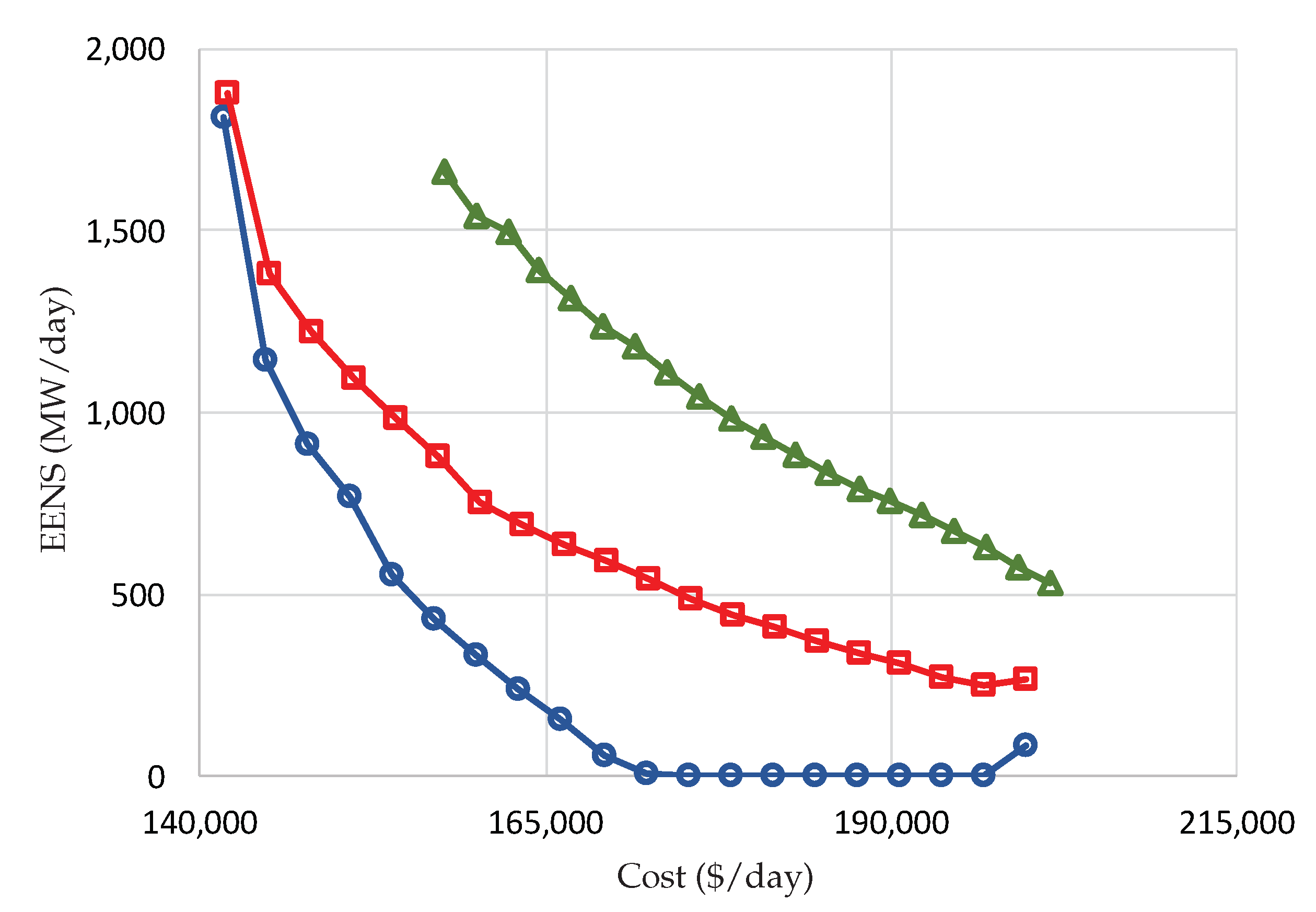
Figure 6 shows the Pareto set of total daily costs vs. EENS for each of the three scenarios. It is observed that the reliability of the RTS increases when the cost of the configurations increases, i.e., the EENS decreases for the most expensive configurations for the three scenarios. With the exception of the least expensive configuration, Scenario 1 shows the best reliability performance followed by Scenario 2 and then Scenario 3. Thus, in Scenario 1, the configurations have a greater ability to meet the load demand than the configurations in Scenario 2 and Scenario 3. The uncertainties of the load demand in Scenario 2 affect the EENS considerably by increasing the standard deviation of the normal distribution that represents the behavior of a node, resulting in an increment of the loss-of-load probability and, as a consequence, the EENS. This effect is increased even more when the uncertainties associated with the production of electricity by the renewable energy producers, i.e., wind and photovoltaic panels, is introduced into the problem.

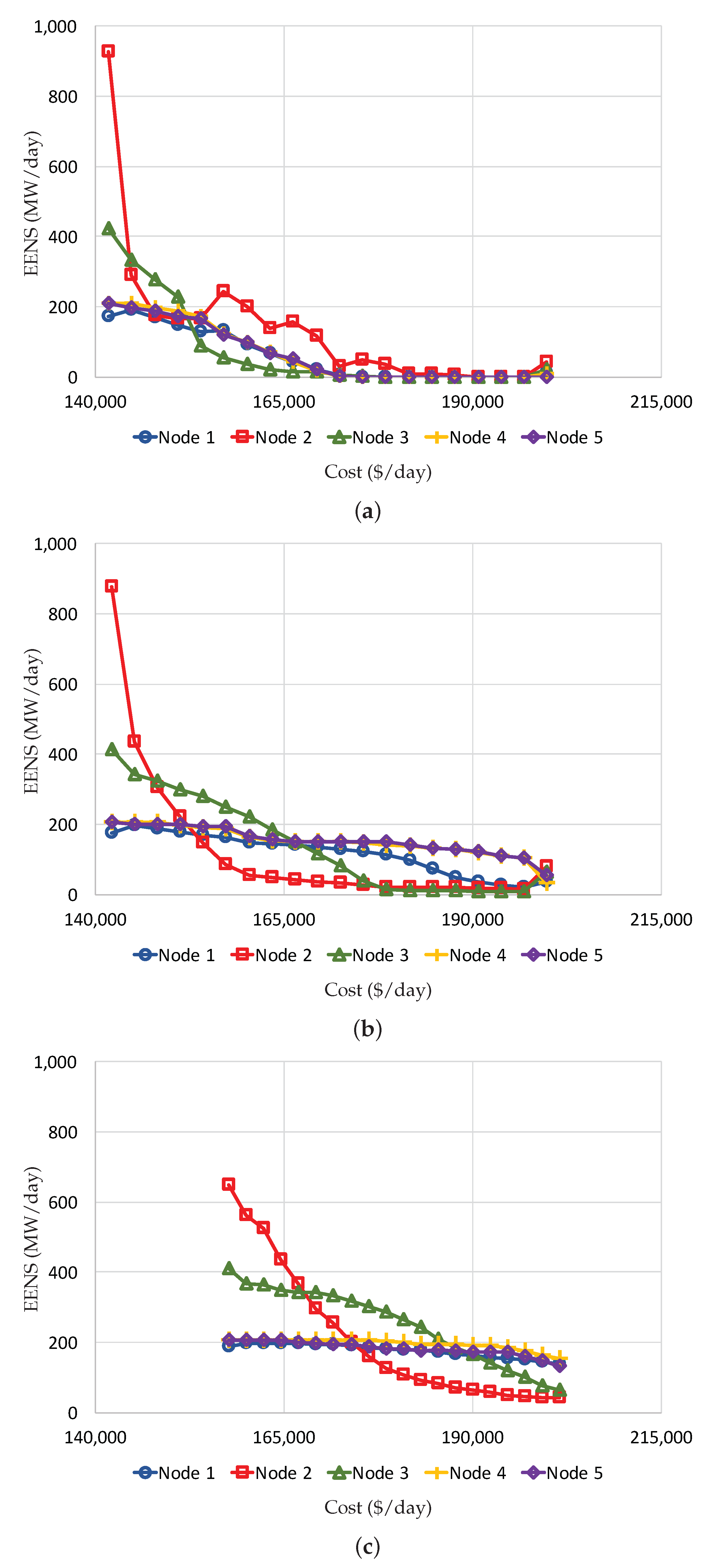
Figure 7 shows the reliability of the different nodes of the RTS for the configurations in the Pareto set for the three scenarios. The value of the EENS at each node is an indicator of the ability of a node, based on the generation at the node and the power flow in and out of the node (transmission), to meet its own load demand. As is seen, the trend of the EENS at each node is similar to that of the overall system. It is observed that Node 2 is the weakest for the less expensive configurations, but is among the strongest for the most expensive configurations in the Pareto set. This behavior is observed also for Node 3. The rest of the nodes have a similar reliability in value and in trend for the different configurations in the Pareto set. For Scenario 2 and Scenario 3, the inclusion of the uncertainties in the load demand results in a faster decrease in the reliability of Node 3 than that for the rest of the nodes. The inclusion of the uncertainties associated with energy production (wind and photovoltaic) makes this effect even more significant, causing the reliability of the network for this scenario to be the lowest. It is also seen that, for Scenario 3, the reliability of Node 1, which is where the wind and photovoltaic producers are added, is not affected by the uncertainties associated with these producers. However, the neighboring nodes (2 and 3) are significantly affected by this uncertainty, showing the effect of the propagation of uncertainties through the transmission lines.

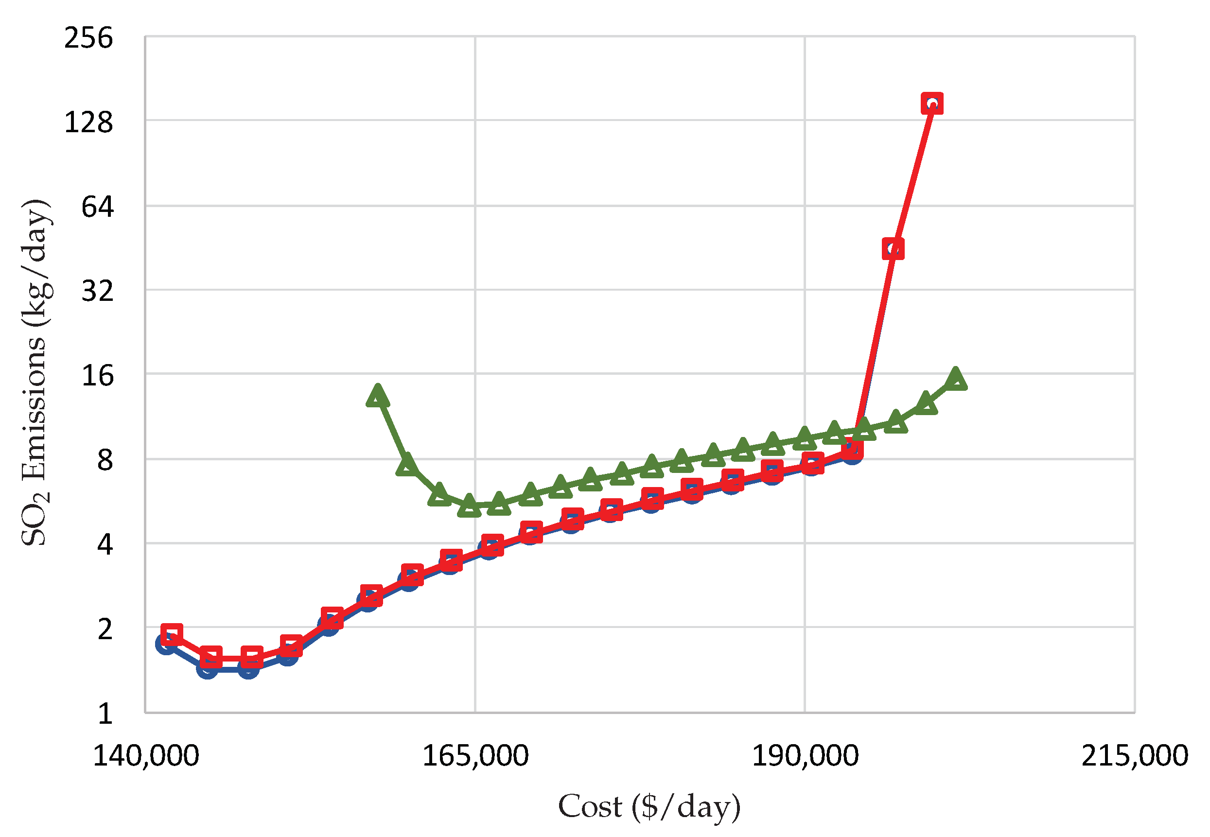
Figure 8 shows the Pareto set of total daily costs vs. SO${}_2$ daily emissions for each of the three scenarios. It is observed that, for the three scenarios, the daily SO${}_2$ emissions decrease for the configurations on the first part of the Pareto set and then increase as the total daily cost of the configurations increases. This is primarily due to the fact that the power production for the three scenarios is dominated by the USC and NGCC at high costs and dominated by the renewable energy producers—i.e., wind, solar, and hydro—at low costs. It is also seen that for Scenario 3, the amount of daily SO${}_2$ emissions is higher than for the other two scenarios. This is because for this scenario, wind and photovoltaic panels produce less electricity than the technologies they replace. Thus, the USC is producing more energy for this scenario than for the other two scenarios. As also sen in this figure, the production of daily SO${}_2$ emissions is almost the same for Scenario 1 and Scenario 2. For these scenarios, NGCC, CT, and RICE producers have a significant impact on the overall daily SO${}_2$ emissions at low costs, and the USC dominates the daily SO${}_2$ emissions at high costs.

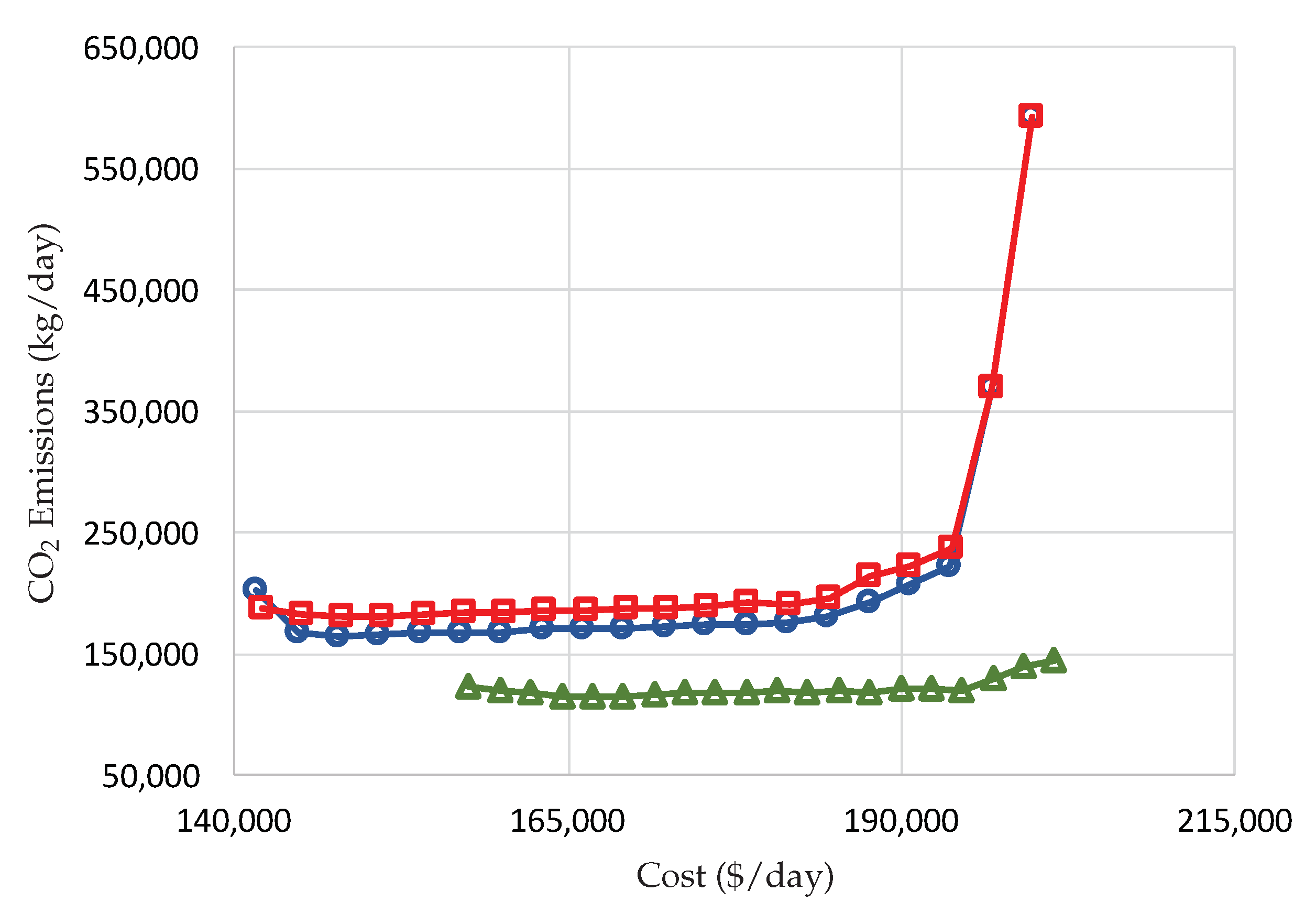
Figure 9 shows the Pareto set of total daily costs vs. CO${}_2$ daily emissions for each of the three scenarios. For the three scenarios, the daily CO${}_2$ emissions decay a small amount and then start to increase as the total daily cost of the configurations increases. This is primarily because renewable energy technologies—i.e., hydro, wind, and photovoltaic producers—dominate the production at low costs and the USC and RICE dominate the production at high costs. It is also observed that for Scenario 3, the amount of daily CO${}_2$ emissions is lower than for the other two scenarios mainly because the configurations in Scenario 3 contain a higher penetration of renewable energy producers such as hydro, wind turbines, and photovoltaic panels. As also seen, including the load uncertainties makes a difference with respect to the daily CO${}_2$ emissions since Scenario 1 has lower values than Scenario 2.

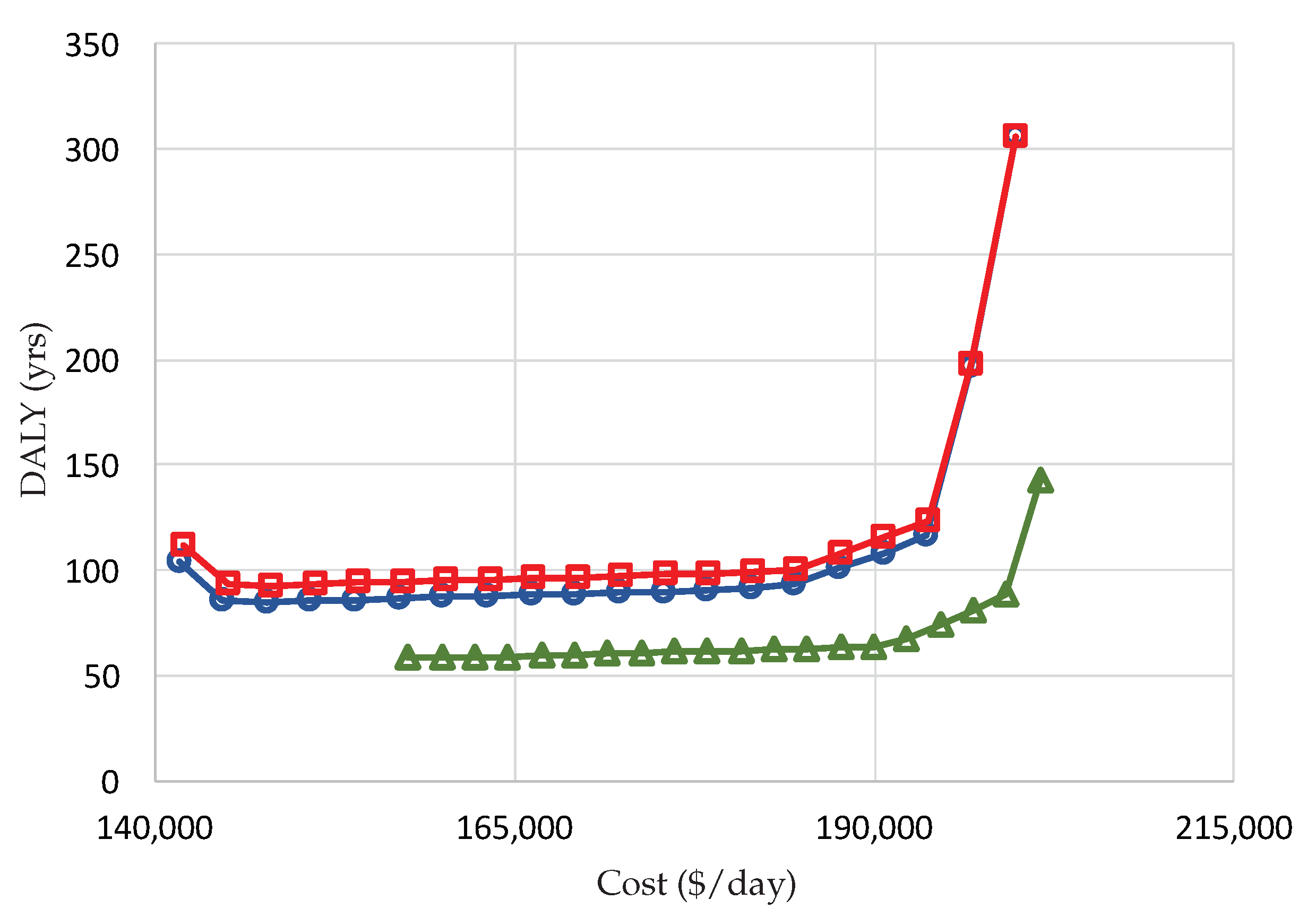
Figure 10 shows the Pareto set of total daily costs vs. DALY for each of the three scenarios. In order to have a more representative result, the DALY is based on a one-year analysis. It is observed that, for the three scenarios, the trend of the DALY is very similar to that for CO${}_2$ emissions, indicating that the DALY is highly dominated by this type of contaminant. Furthermore, it is seen that for Scenario 1 and Scenario 2, the DALY increases as the total daily cost of the configurations increases. This is primarily because renewable energy technologies—i.e., hydro, wind, and photovoltaic producers—dominate the production at low costs and the USC with its NO${}_{\mathrm{x}}$-DALY, and RICE and NGCC with their CO${}_2$-DALY dominate the region of high costs. Furthermore, including the load uncertainties makes a difference with respect to the DALY since Scenario 2 has somewhat higher values than Scenario 1. It is also seen that for Scenario 3, the DALY is lower than for the other two scenarios and remains almost constant for all configurations except for the most expensive ones when the DALY increases. This is primarily because the configurations in Scenario 3 contain more renewable energy producers than do Scenario 1 and Scenario 2.

Figure 11 shows the Pareto set of total daily costs vs. daily exergy production, which is directly proportional to the exergetic efficiency of the RTS, for each of the three scenarios. As seen in the figure, the daily exergy production decays a small amount in the first part of the Pareto set for the three scenarios and then starts to increase as the total daily cost of the configurations increases. This is primarily because the most efficient technologies such as NGCC and CT dominate the production at low costs and the less efficient USC and RICE dominate the production at high costs. Furthermore, as seen in the figure, including the load uncertainties makes a difference with respect to the daily exergy production since Scenario 2 has higher values than Scenario 1. It is also observed for Scenario 3 that the amount of daily exergy production is lower than for the other two scenarios mainly because the configurations in Scenario 3 contain extra renewable energy producers, which replace two fossil fuel-based producers, i.e., RICE and CT.

6. Conclusions

A generation-transmission reliability approach based on the mixture of normals approximation and its incorporation into a sustainability assessment framework for power network planning is proposed. The IEEE-RTS is used as a test system to evaluate the effectiveness of the methodology proposed.

The EENS objective function used here is based on a probabilistic as opposed to a deterministic approach, which can also account for the effects of catastrophic events as intrinsic to the system. The EENS provides detailed information about the producers and transmission lines during the synthesis/design optimization of power networks. Furthermore, the use of a MONA as the basis for the reliability framework makes the analysis and optimization of power networks much simpler than using a Monte Carlo approach, which in fact would render the optimization problem insoluble.

The inclusion of the cost for the possible construction of a new transmission line into the total daily cost, together with the capital cost and fixed and variable costs of producers considerably impacts the design of the power network configurations. The SO${}_2$ daily emissions objective function favors the use of renewable energy producers and a relatively clean fossil technology such as NGCC for the most expensive configurations. However, because of the intermittent generation of wind and photovoltaic producers, the coal plant has to increase its power production for the less expensive configurations, increasing the overall production of SO${}_2$ emissions. The CO${}_2$ emissions objective function also gives preference to renewable energy technologies, as well as technologies such as RICE and USC. The Disability Adjusted Life Year (DALY) objective function as well prefers the use of renewable energy producers. The exergetic efficiency of the RTS objective function favors the use of producers based on natural gas such as NGCC and CT.

An increase in the penetration of renewable energy producers has some positive impact on the synthesis/design optimization of power networks under sustainability considerations. This is especially important in the reduction of CO${}_2$ emissions (environmental pillar), in the disability adjusted life years of the population due to the emission of contaminants from local power plants (social pillar), and in the decrease of the use of fossil fuel in the network (technical pillar).

The cost (economic pillar) of using renewable energy producers is higher when compared with fossil fuel-based producers. This is not surprising since renewable energy producers are still maturing. However, it is expected that this gap will eventually be reduced.

The uncertainties associated with the generation of wind and photovoltaic producers reduce significantly the reliability of the power network. This is a disadvantage, which is only associated with these two types of renewable energy technologies due to their dependency on weather conditions. Nonetheless, it is important to consider wind and photovoltaic producers as players in a power network since they are the most mature of all the non-thermal renewable energy technologies.

Finally, the results presented here suggest that, for a reliability analysis of power networks, it is important to consider in a single methodology as many of the sources of uncertainties associated with the network as possible. These include not only those for the generation, transmission, and load demand considered here, but those attributed to other sources as well, such as, for example, those resulting from power distribution, emergency infrastructure interactions, unexpected catastrophic events, etc. Efforts to include these additional effects is left for future work.