Thermo-Electric Energy Storage with Solar Heat Integration: Exergy and Exergo-Economic Analysis

Abstract

A Thermo-Electric Energy Storage (TEES) system is proposed to provide peak-load support (1–2 daily hours of operation) for distributed users using small/medium-size photovoltaic systems (4 to 50 kWe). The purpose is to complement the PV with a reliable storage system that cancompensate the produc tivity/load mismatch, aiming at off-grid operation. The proposed TEES applies sensible heat storage, using insulated warm-water reservoirs at 120/160 °C, and cold storage at −10/−20 °C (water and ethylene glycol). The power cycle is a trans-critical CO₂ unit including recuperation; in the storage mode, a supercritical heat pump restores heat to the hot reservoir, while a cooling cycle cools the cold reservoir; both the heat pump and cooling cycle operate on photovoltaic (PV) energy, and benefit from solar heat integration at low–medium temperatures (80–120 °C). This allows the achievement of a marginal round-trip efficiency (electric-to-electric) in the range of 50% (not considering solar heat integration).The TEES system is analysed with different resource conditions and parameters settings (hot storage temperature, pressure levels for all cycles, ambient temperature, etc.), making reference to standard days of each month of the year; exergy and exergo-economic analyses are performed to identify the critical items in the complete system and the cost of stored electricity.

1. Motivation and Introduction

The increasing market penetration of renewables is challenging the current structure of electrical grids [1]. Most renewables require a balance between production and load; production depends on highly stochastic resources (wind, wave energy) or is subject to daily cycles (solar). To solve the dispatchability issue, several countries are still obliged to use fossil fuels, with the situation aggravated by occasional use of plants and requiring operation under peak-load switch mode. Another way to solve the problem is to associate energy storage with the increasing use of renewables; today, the largest applied energy storage is still pumped hydro, which is possible only under favorable conditions of availability of sites and hydro resource.

On the other hand, the market is experiencing an increasing diffusion of off-grid or locally connected smart-grid user communities. These are at present expensive solutions, based on small-scale distributed energy systems; only for specific situations are these solutions practiced, such as on islands or in remote locations where the connected grid infrastructure is missing (and often electricity is provided by expensive diesel generators). Off-grid or small connected smart-grids today represent a challenge, where new advanced solutions trying to satisfy community energy needs (power, heat, and possibly other attractive products or services) can be investigated.

Within this context, the idea of developing medium-size energy storage (ES) systems becomes attractive. These ES should couple flexibility (providing power and possibly heat or cold), reliability, capability of load matching, and life cycle durability. These features are not easily achievable by modern batteries, which are the preferred solutions of smart-grid promoters but present several bottlenecks when applied under these stringent conditions. The consequence is that even when backing up a renewable energy system (solar, wind) with a substantial battery pack, it is in general necessary to include in the package a diesel generator for off-grid power.

The portfolio of ES technologies is quite wide, as it embraces different concepts, such as pumped-storage hydroelectricity (PHS), flywheel storage (FS), batteries, compressed air energy storage (CAES), liquid air energy storage (LAES), or other gas storages using hydrogen or CO₂, as well as super-capacitor or chemical storage [2]. All these solutions are challenged by the increasing share of electricity generation by renewables. Specifically, each technology presents advantages and drawbacks, which make the correct selection of storage systems deeply dependenton the application. Among the selection criteria are relevant aspects are the cost of the system, the total efficiency, the energy density, and the power rating. In [3], a comprehensive comparison of the various ES technologies, including both technical and economical features, is carried out.

PHS, as well as CAES, are subject to geographical constraints; therefore, they can only play a relevant role for places where the geographical sites are suitable [4]. The main issue of battery storage is the limited life cycle [5], while chemical storage certainly represents the ultimate solution for managing long-term unavailability of renewables such as wind or wave power, but is highly penalized by a limited round-trip efficiency. In this frame, Thermo-Electric Energy Storage (TEES) [4,5,6] represents an interesting solution in the general context of ensuring dispatchability to energy systems based on renewables. A TEES system is basically composed of two sensible heat/cold accumulators, between which temperature levels a heat engine works. The temperature levels are then re-charged by a heat pump cycle.

Multi-MW TEES cycles have been proposed, often using a trans-critical CO₂ cycle as the power cycle [5,6,7,8]. Another variant of the TEES is that using the Brayton cycle as power cycle, with air [9], Argon, or other noble gases [10,11] as working fluids.

In the literature, TEES systems are not widely studied, especially when considering the whole integration process of solar energy both as heat input (in the discharge cycle) and as electricity input (in the charging cycle, providing the work input for compressors operation). Particularly, in [12], a novel pumped thermal electricity storage (PTES) system with heat integration was proposed. The main novelty was the introduction of an auxiliary heat source, which enhances the efficiency of the system. In [13], an overview on TEES is presented, dealing also with thermo-economic evaluation. A comprehensive thermo-economic analysis of a TEES is developed in [14], where a round-trip efficiency of 64% was obtained for a 50 MW power plant with an initial investment of 34 M$. Another thermo-economic analysis is proposed in [15], where the TEES is supported by the use of solar collectors.

On the whole, relevant research work has been dedicated to TEES. Nonetheless, there is still a gap in the literature in comprehensive assessments of solar-aided TEES systems; dealing with a system using exchange of heat and power, an exergo-economic analysis is recommended as the best tool for studying parametric optimization of the system.

In the present study, a thermodynamic and exergo-economic analysis of a TEES is performed, with solar panels and photovoltaic (PV) integration in the charging and discharging cycles. Two different representative case studies of geographical sites are presented and discussed (Crotone and Pantelleria in Italy). The thermodynamic cycles were designed and optimized, from an exergy and exergo-economic perspective, to address the highest possible performance for a variable heat input depending on the availability of the solar resource.

2. TEES Description and Methods of Analysis

2.1. Description of TEES

In the present study, focusing on ESs assisting medium-size photovoltaic systems (PV), which depend on the daily availability of solar radiation, sensible heat or cold accumulation is practiced. The TEES here proposed is based on three separate systems: a power cycle, a heat pump, and a refrigeration cycle. The heat pump and the refrigeration cycle are working during the charging phase, using solar energy converted into thermal and electric energy.

As shown in Figure 1 and Figure 2, during daylight operation the hot and cold reservoirs are charged using respectively a heat pump and a refrigeration unit. After daylight, a power cycle (Figure 3) operating between the hot, medium temperature, and cold reservoirs produces the necessary power for the community. The hot and cold reservoirs are available for flexible energy use: hot sanitary water and heating can be assisted by the hot and/or medium temperature reservoir, while in hot periods the cold reservoir can be connected to the domestic comfort cooling network.

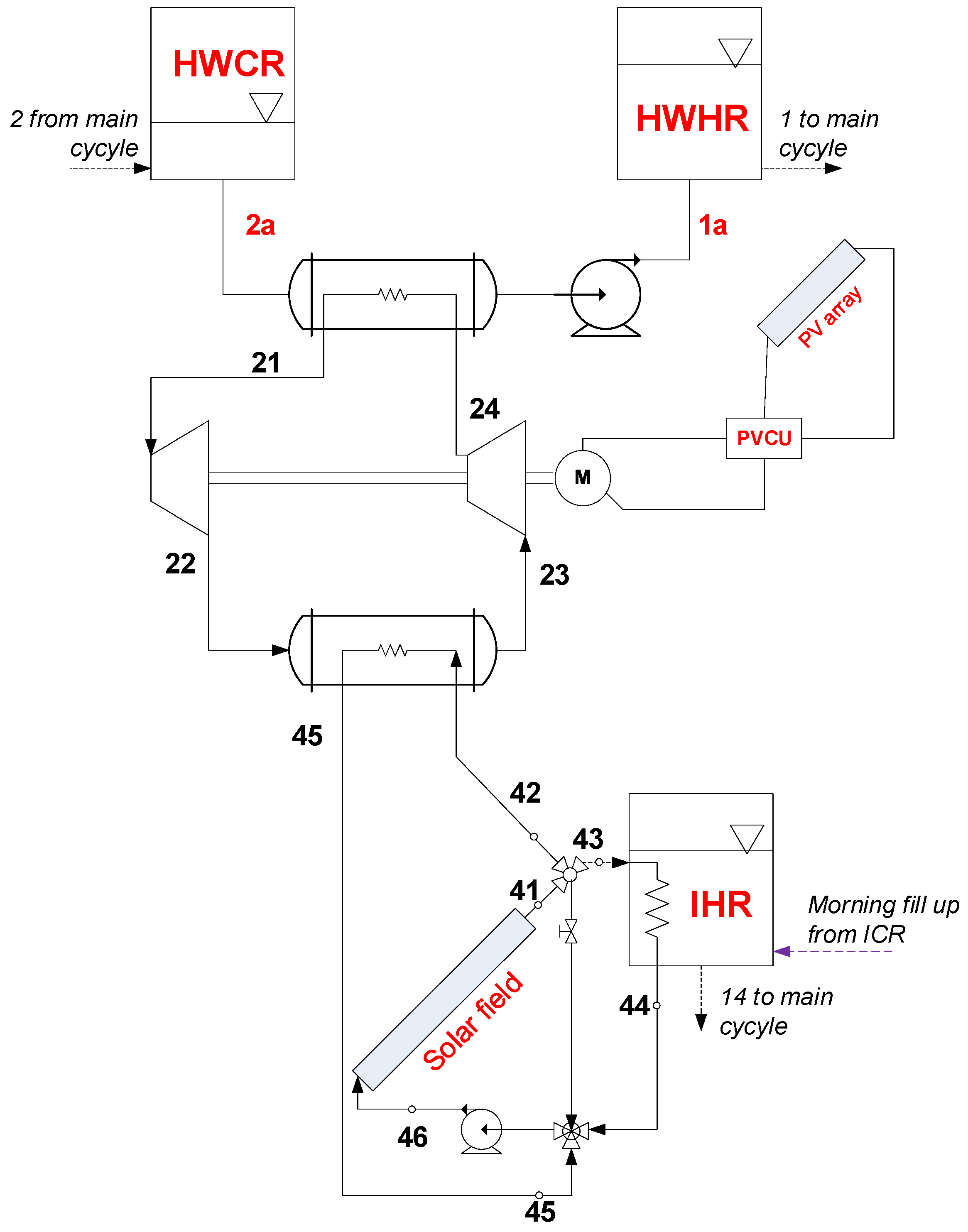
The schematic of the heat pump cycle is shown in Figure 1. The purpose of the heat pump cycle is to restore the required sensible heat in the HWHR. To achieve the required temperature level (145 °C), the proposed heat pump works with the architecture of a supercritical CO₂ cycle. The use of a supercritical cycle, which is mostly due to the required temperature levels, allows a proper matching of the heat capacities of the stored water (pressurized at 1800 kPa) and of the heat pump working fluid (supercritical CO₂).

With respect to a traditional heat pump, an expander is proposed in place of the throttling valve (21–22), which allows an increase in COP values [16]. Moreover, the heat pump cycle is deeply integrated with solar panels and PV collectors. Specifically, the evaporator temperature is determined by the operation of the thermal collectors of the solar field, through a three-way valve, which also allows the setting of the optimal temperature of an intermediate hot reservoir (IHR).

Finally, the required compressor work (23–24, partly supported by the expander), is provided by a PV array, which thus allows a complete solar TEES integration.

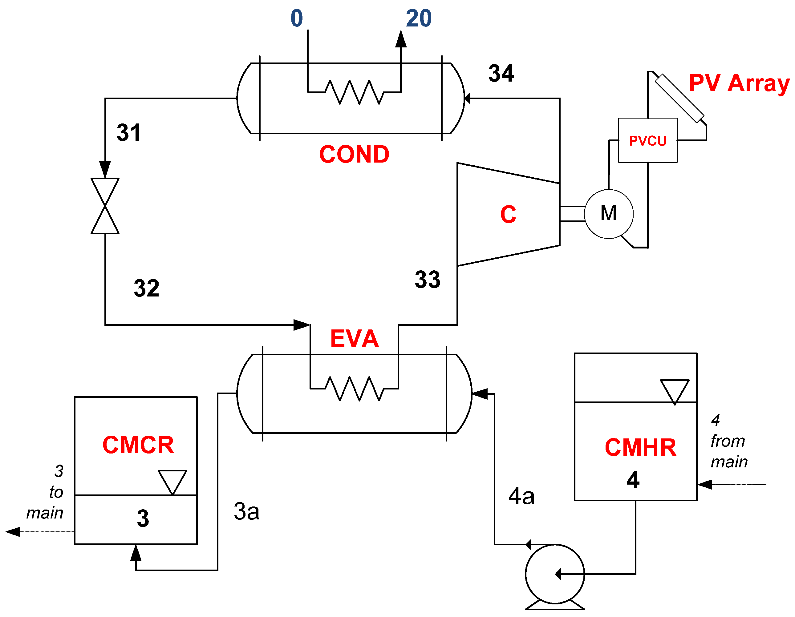
The schematic of the refrigeration cycle is shown in Figure 2. The objective of the refrigeration cycle is to restore the cold energy in the CMCR, reducing the temperature of the water-ethylene glycol mixture, taken from the CMHR. The presence of a low-temperature cold storage is of paramount importance if suitable round-trip efficiency is coveted.

The condenser of the refrigeration cycle rejects heat to the environment (0–20). The ambient temperature is a very important parameter for the refrigeration cycle, as lower ambient temperatures allow higher coefficient of performance (refrigeration cycle evaporator-condenser temperature becomes closer). Different fluids (R134a, R717, R1233zd(E), R404a) were investigated as possible choices for the refrigeration cycle working fluid. The most favorable solution resulted in a subcritical R134a cycle. As for the heat pump, operation of the compressor of the refrigeration cycle is provided by surplus power available from the PV solar field.

The opportunity of using a cold storage represents a considerable advantage for the power cycle, as it can work across a higher temperature difference, therefore allowing a superior performance of the power cycle. For this purpose, the use of water mixtures with suitable anti-freeze additives (such as Ethylene Glycol or Calcium Chloride) is recommended. The cold storage is restored to the initial low temperature during the charging mode operation, using the proposed subcritical R134a refrigeration cycle.

The assumed values of the reference variables for the heat pump and the refrigeration cycles are resumed in

Table 1. Reference design parameters for the Heat Pump and Refrigeration Cycles.

Variable	Value
Heat Pump Cycle
ΔTCO2-HW = T21 − T2a	5 °C
pmin, HP	13500 kPa
ΔTsolar-CO2 = T42 − T23	5 °C
Refrigeration Cycle
ΔTCOLD = T31 − T0	10 °C
ΔTEVA = T3a − T32	5 °C

.

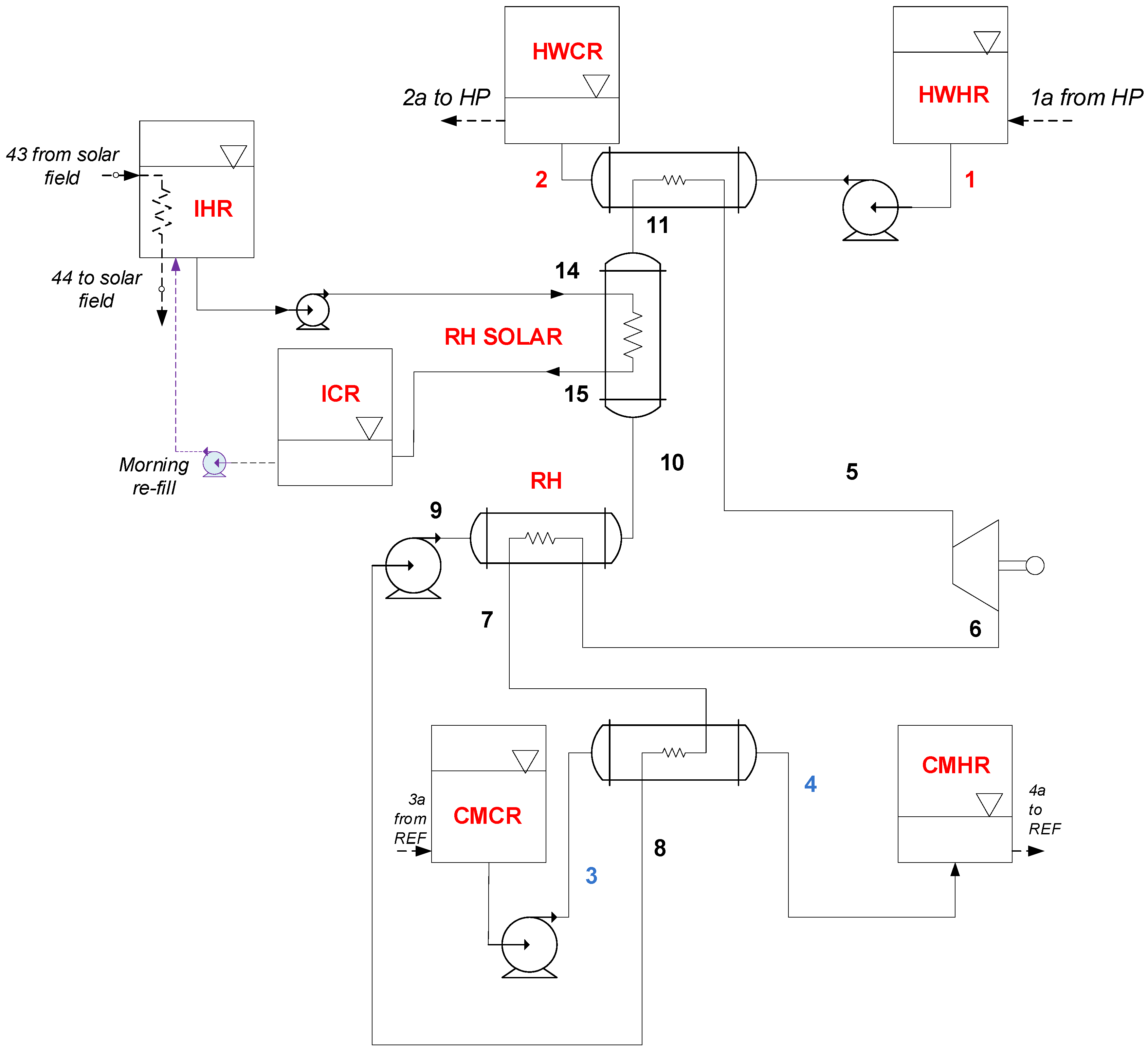
The trans-critical CO₂ power cycle (Figure 3) is a common solution for TEES applications: in fact, CO₂ is particularly attractive for the temperature levels involved (high and low temperature), and the trans-critical choice allows a good matching of heat capacities for the hot resource. The basic idea is to use as far as possible the same components for the heat pump and the trans-critical CO₂ cycle through an appropriate commutation of configuration valves. This mode of operation is certainly affected by the different operational time for storage and power modes and—consequently—by the different mass flow rates; moreover, a solar-aided TEES experiences different heat input conditions throughout the year as well as throughout the day.

The proposed system uses a simple solution of sensible heat liquid reservoirs for the hot and cold storage: even though there are several limitations with this technology, use of simple insulation materials and the possibility of quickly adjusting the mass flow rates in order to match the heat capacities of both charging and discharging cycles make this solution attractive for the power size here considered. An intermediate temperature reservoir (IHR and ICR) charged by solar heat allows preheating of the working fluid, thus enhancing the efficiency of the system.

The selection of the power cycle operating temperatures, as well as the optimal conditions of the hot, intermediate and cold reservoirs (HWCR, HWHR, ICR, IHR, CMCR, CMHR), is the outcome of a parametric analysis, taking into account not only the power cycle but also the two recharging cycles (heat pump and refrigeration cycle).

Water in the additional, intermediate temperature reservoir (IHR) is warmed up to the desired temperature by solar heat during the charging phase. Exploiting heat from the IHR accumulator makes the discharging phase independent of transient meteorological conditions.

Referring to the Hot and Intermediate twin reservoirs, it is possible to place the vessels at different elevation levels to take advantage of buoyancy to design a system using no pumps for fluid displacement. However, at this stage of research, it was assumed that the circulation pumps between all twin tanks should cover a 4-m circuit head loss. The design pumping power for the assemblies was calculated accordingly, and results very limited.

The power cycle operating parameters under design conditions are summarized in

Table 2. Power cycle design operating parameters.

Variable	Value
T1, T2 (HWR)	95/145 °C
pHWR, pIHR, pCMR	1800/100/100 kPa
${\dot{\mathrm{m}}}_{\mathrm{HW}}$	1 kg/s
T14, T15 (RH-SOLAR)	95/40 °C
p5	12,000 kPa
ΔTHOT = T1 − T5 = ΔTSOLAR = T14 − T11	5 °C
ΔTCOLD = T8 − T3	10 °C
T3, T4 (CWR)	−20/−10 °C
εRH	0.8
ηt, ηp	0.9/0.8
Operation Time (Power Cycle)	h

.

A crucial issue when considering a system that relies solely on an energy source of intermittent availabilitysuch assolar radiation is its control management. In the present case, the system is preliminarily assessed assuming that it should be able to provide a constant power output for a limited time in the evening (e.g., 1 h), but control should indeed address complete daily resource and load management in a practical application. In particular, the charging phase is burdened with considerable deviations from design loads in the early morning and evening hours, as is typical for all systems relying on the solar resource. Several control paths could be tested and then potentially implemented. In the early morning and late afternoon operation, compressors could be supported by a small-capacity battery pack, or use limited grid assistance. Moreover, the compressors can be equipped with a variable-speed drive to follow the variable load conditions; and multiple parallel-arranged sets of compressors can be proposed for TEES systems of large capacity, with step-by-step load control. An automated control system based on control routines adapting the operational parameters (pressures, temperatures) to changing conditions can also be proposed. As stated before, the aim of this paper is to evaluate the possible application of solar energy-integrated TEES and to demonstrate its performance and individuate a pathway for possible improvement. In this light, control issues are not explicitly dealt at the present stage of research.

2.2. Power Cycle-Thermodynamic Model Equations

In the following, the main model equations are presented only for the power cycle, as the heat pump and refrigeration cycle are conventional units (with the main novelty of solar-thermal assistance for the heat pump, which is dealt in the following).

The operation of the power cycle is determined in terms of heat input by the pre-set conditions at the HWHR in terms of flow rate ${\dot{\mathrm{m}}}_{\mathrm{HW}}$ as shown in Equation (1):

$${\dot{\mathrm{Q}}}_{12}={\dot{\mathrm{m}}}_{\mathrm{HW}}\left({\mathrm{h}}_1-{\mathrm{h}}_2\right)$$

(1)

Knowing the conditions of the hot resource and assuming the minimum possible temperature difference, it is possible to calculate the working fluid flow rate through Equation (2).

$${\dot{\mathrm{m}}}_{\mathrm{WF}}=\frac{{\dot{\mathrm{Q}}}_{12}}{\left({\mathrm{h}}_5-{\mathrm{h}}_{11}\right)}$$

(2)

The temperature and enthalpy conditions at point 11 are defined by the heat extraction from the solar field resource Equation (3), which allows an increase of the system efficiency, as the working fluid is pre-heated before the high-temperature heat exchanger:

$${\mathrm{T}}_{11}={\mathrm{T}}_{14}-\Delta {\mathrm{T}}_{\mathrm{solar}}$$

(3)

The turbine power output is obtained through the application of Equation (4), assuming a turbine isentropic efficiency of 0.9 at design point:

$${\dot{\mathrm{W}}}_{\mathrm{t}}={\dot{\mathrm{m}}}_{\mathrm{WF}}\left({\mathrm{h}}_5-{\mathrm{h}}_6\right)={\dot{\mathrm{m}}}_{\mathrm{WF}}\left({\mathrm{h}}_5-{\mathrm{h}}_{6\mathrm{s}}\right)·{\mathsf{\eta }}_{\mathrm{T}}$$

(4)

The application of energy balance at the re-heater Equation (5), assuming a re-heater efficiency of 0.8, allows setting of the re-heater heat duty:

$${\mathsf{\epsilon }}_{\mathrm{RH}}=\frac{{\dot{\mathrm{Q}}}_{\mathrm{RH}}}{{\dot{\mathrm{Q}}}_{\mathrm{RH},\mathrm{MAX}}}=\frac{{\dot{\mathrm{m}}}_{\mathrm{WF}}·\left({\mathrm{h}}_6-{\mathrm{h}}_7\right)}{{\dot{\mathrm{m}}}_{\mathrm{WF}}·\left({\mathrm{h}}_6-{\mathrm{h}}_{7\min }\right)}=\frac{{\dot{\mathrm{m}}}_{\mathrm{WF}}·\left({\mathrm{h}}_{10}-{\mathrm{h}}_9\right)}{{\dot{\mathrm{m}}}_{\mathrm{WF}}·\left({\mathrm{h}}_6-{\mathrm{h}}_{7\min }\right)}$$

(5)

where h_{7 min} is evaluated at T_{7 min} = T₉ and p₇ = p₆.

The CO₂ supercritical condenser is cooled using the cold stored in the reservoirs, thus allowing the setting of the low-pressure level of the discharging cycle Equation (6):

$${\dot{\mathrm{Q}}}_{34}={\dot{\mathrm{m}}}_{\mathrm{CW}}\left({\mathrm{h}}_4-{\mathrm{h}}_3\right)={\dot{\mathrm{m}}}_{\mathrm{WF}}\left({\mathrm{h}}_7-{\mathrm{h}}_8\right)$$

(6)

which, once T₄ and T₃ are given, can be solved for ${\dot{\mathrm{m}}}_{\mathrm{WF}}$. Finally, the calculation scheme of the cycle is closed by the calculation of the trans-critical CO₂ pump through Equation (7), assuming a pump isentropic efficiency of 0.8:

$${\dot{\mathrm{W}}}_{\mathrm{P}}={\dot{\mathrm{m}}}_{\mathrm{WF}}\left({\mathrm{h}}_9-{\mathrm{h}}_8\right)={\dot{\mathrm{m}}}_{\mathrm{WF}}\left({\mathrm{h}}_{9\mathrm{s}}-{\mathrm{h}}_8\right)/{\mathsf{\eta }}_{\mathrm{p}}$$

(7)

Furthermore, it is possible to calculate the required volumes of the reservoirs: one hour of power cycle autonomy is assumed. Their size should satisfy the heat demand of three cycle heat exchangers. The sizing of the reservoirs volume is also fundamental for the off-design analysis.

Once all the temperatures, flow rates, and heat duties are known, the heat exchangers sizes are determined by means of the Péclet Equation (8).

$${\dot{\mathrm{Q}}}_{\mathrm{k}}={\left(\mathrm{UA}\right)}_{\mathrm{k}}·\Delta {\mathrm{T}}_{\lg ;\mathrm{k}}$$

(8)

2.3. Solar Integration

Solar integration with the TEES uses a combination of thermal and photovoltaic conversion. Solar thermal collectors are supporting the evaporator in the heat pump system and, simultaneously, are charging the intermediate reservoir (IHR). Meanwhile, PV panels are providing electric energy to drive compressors in the heat pump and refrigeration cycles sections. At the design stage, a crucial issue is the sizing of both the solar thermal collectors and the PV fields. Their energy output is strictly dependent on the local meteorological conditions. Knowing these for a chosen location, the desired size of the two fields can be determined. The sizing was done through a one-reference-day quasi-dynamic model approach for the given location.

A commercially available flat-plate solar collector was considered for the solar-thermal field. The efficiency of solar collectors (${\mathsf{\eta }}_{\mathrm{sc}}$) depends on incoming radiation (${\mathrm{G}}_{\mathrm{sloped}}$), ambient temperature, and working fluid temperature increase; applying the typical 2^nd order Bliss-equation [17]:

$${\mathsf{\eta }}_{\mathrm{sc}}={\mathsf{\eta }}_{\mathrm{o}}-\left({\mathrm{a}}_1+{\mathrm{a}}_2\Delta \mathrm{T}\right)\frac{\Delta \mathrm{T}}{{\mathrm{G}}_{\mathrm{sloped}}}$$

(9)

The coefficients ${\mathsf{\eta }}_{\mathrm{o}}$, ${\mathrm{a}}_1$ and ${\mathrm{a}}_2$ (

Table 3. Solar-thermal collector fields operating parameters.

Variable	Description
Location	Crotone, Italy
Month for reference day	May
Slope of solar collector	45° towards South
η0	0.719
a1	1.45 W/(m2K)
a2	0.0051 W/(m2K2)
Asc	1.6 m2
T41 = T42 = T43	95 °C
ΔTHTF= T42 − T45= T43 − T44	10 K
Collectors arrangement	Parallel in 10 rows

) are commonly provided by the manufacturer of the collector. ΔT is the temperature difference between the average Heat Transfer Fluid (HTF) temperature and the ambient temperature. The HTF inlet and outlet temperatures are assumed as known at the design conditions.

The useful heat gain from the solar field is shared between the heat pump evaporator demand and the IHR tank. In this last stage, water is warmed up to a fixed temperature to be used during the power cycle operation. The solar-thermal field arrangement was shown in Figure 1 together with the heat pump assembly.

The solar field surface A and, thus, the number of solar collectors, was found iteratively requiring that the daily solar heat yield can satisfy the heat pump and IHR tank energy needs. The applied procedure is summarized in the set of Equations (10) and (11). The procedure is formally started at 7 a.m., but depending on the month and weather conditions the effective heat accumulation can begin later. It is assumed that collectors are arranged in parallel in 10 equal rows. Thus, the task is to calculate the number of collectors in a row:

$$\underset{7:00}{\overset{7:00+{\mathsf{\tau }}_{\mathrm{charge}}}{{\displaystyle \int }}}{\dot{\mathrm{Q}}}_{\mathrm{sc}}\mathrm{d}\mathsf{\tau }={\mathrm{N}}_{\mathrm{sc}}{\mathrm{A}}_{\mathrm{sc}}\underset{7:00}{\overset{7:00+{\mathsf{\tau }}_{\mathrm{charge}}}{{\displaystyle \int }}}{\mathsf{\eta }}_{\mathrm{sc}}{\mathrm{G}}_{\mathrm{sloped}}\mathrm{d}\mathsf{\tau }$$

(10)

$$\underset{7:00}{\overset{7:00+{\mathsf{\tau }}_{\mathrm{charge}}}{{\displaystyle \int }}}{\dot{\mathrm{Q}}}_{\mathrm{sc}}\mathrm{d}\mathsf{\tau }=\underset{7:00}{\overset{7:00+{\mathsf{\tau }}_{\mathrm{charge}}}{{\displaystyle \int }}}{\dot{\mathrm{Q}}}_{\mathrm{evapHP}}\mathrm{d}\mathsf{\tau }+{\mathrm{Q}}_{\mathrm{IHR}}$$

(11)

The amount of heat required by the heat pump evaporator is a function of HWR volume. The design conditions of the main cycle determine the need for warming and moving the total volume of water, which also depends on the charging time (${\mathsf{\tau }}_{\mathrm{charge}}$). On the other hand, the solar-thermal input should also assure warming the water in IHR tank to the required temperature. Considering these constraints, both the number of solar collectors and the charging time can be determined. The design assumptions for this section are collected in Table 3.

At the same time, the number of PV panels to satisfy the net compressors power must be defined. Commercially available polycrystalline modules were considered. A TRNSYS (http://www.trnsys.com/) model provided the power output distribution from one polycrystalline Schott SAPC 165 [18] PV module for the reference day of May. Knowing the electric energy needed by the compressors during the whole charging time, the number of PV panels required to produce that daily work output can be calculated.

$$\underset{7:00}{\overset{7:00+{\mathsf{\tau }}_{\mathrm{charge}}}{{\displaystyle \int }}}\left({\dot{\mathrm{W}}}_{\mathrm{c};\mathrm{ref}}+{\dot{\mathrm{W}}}_{\mathrm{c};\mathrm{HP}}-{\dot{\mathrm{W}}}_{\exp ;\mathrm{HP}}\right)\mathrm{d}\mathsf{\tau }={\mathrm{n}}_{\mathrm{PV}}\underset{7:00}{\overset{7:00+{\mathsf{\tau }}_{\mathrm{charge}}}{{\displaystyle \int }}}{\dot{\mathrm{W}}}_{\mathrm{module}}\mathrm{d}\mathsf{\tau }$$

(12)

2.4. Off-Design Simulation

The analysis under off-design conditions is of primary importance for solar energy conversion systems to evaluate the dynamic behaviour of the whole system and the performance over the year. Once all the components are sized, the off-design analysis investigates the capability of the charging cycles to load the reservoirs under variable meteorological conditions. The off-design analysis is built upon a time-forward simulation, which requires a time discretization. The evolutionary variable time step (${\mathsf{\tau }}_{\mathrm{i}}$) is physically determined as the time needed by the volume of HTF to flow through the solar field arranged in 10 rows (represented by the calculated length L).

$${\mathsf{\tau }}_{\mathrm{i}}=\frac{\mathrm{L}}{{\mathrm{V}}_{\mathrm{av},\mathrm{i}}}$$

(13)

The velocity ${\mathrm{V}}_{\mathrm{av},\mathrm{i}}$ is calculated step by step from the mass flow rate in the single collector considering an average density of the HTF and the solar collector pipe diameter, as in Equation (14). This estimate is indeed simplified, and it assumes that the HTF velocity in one single collector is maintained in the whole solar field.

$${\mathrm{V}}_{\mathrm{av},\mathrm{i}}=\frac{{\dot{\mathrm{m}}}_{\mathrm{HTF},\mathrm{i}}}{{\mathsf{\rho }}_{\mathrm{av},\mathrm{HTF}}·\mathsf{\pi }\frac{{\mathrm{d}}_{\mathrm{pipe}}{}^2}{4}}$$

(14)

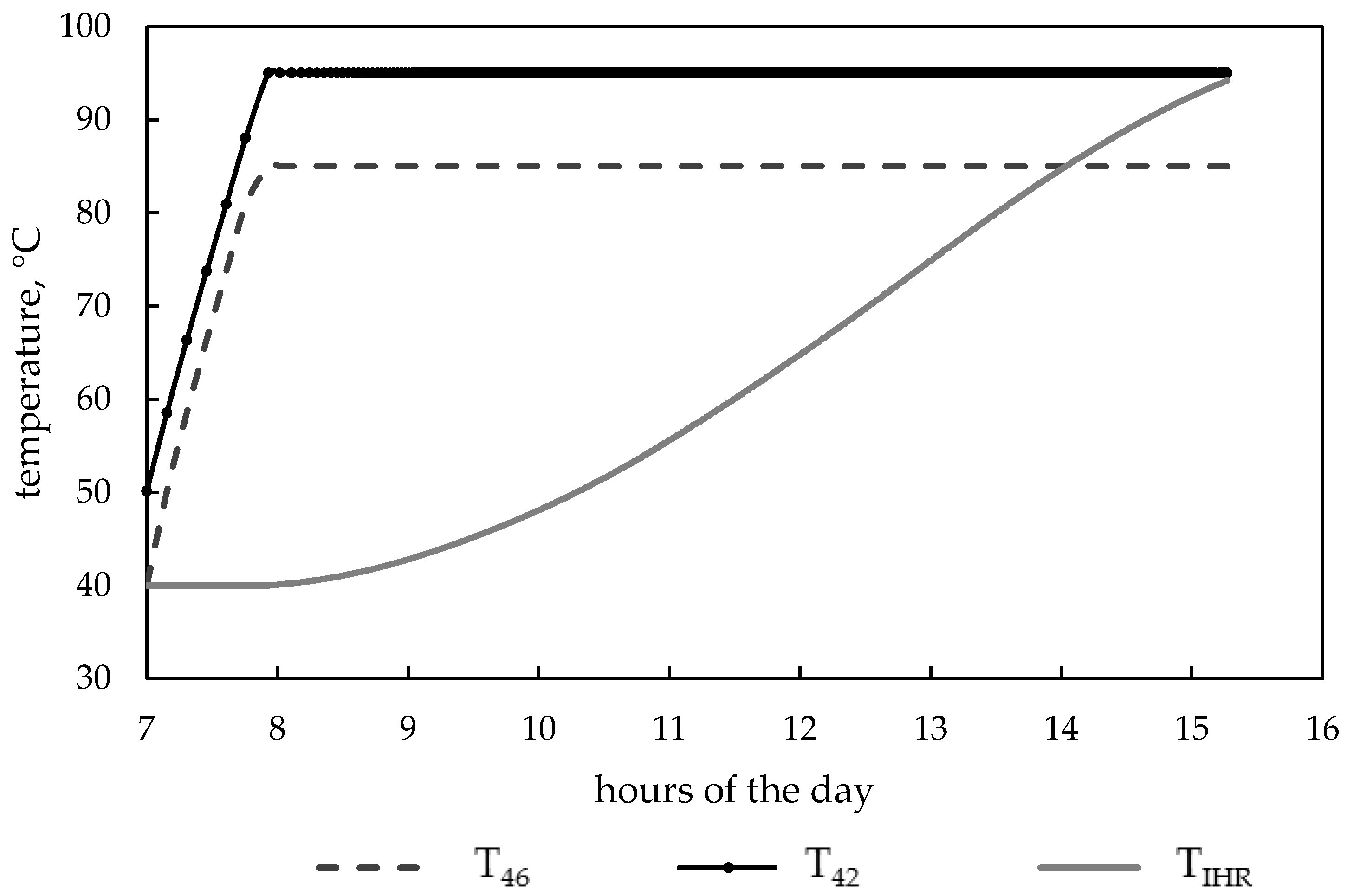
Knowing the hourly meteorological conditions (i.e., the solar radiation on the inclined collectors’ surface), the simulation starts at 7:00 with the solar field warming-up cycle. It is assumed that the initial temperature of the HTF is 40 °C (thanks to the insulated intermediate ICR reservoir where water is stored after the last heat delivery from the power cycle). The HTF circulates in the closed-loop solar field until the outlet temperature reaches 95 °C. At this temperature level, the useful heat gain can be exploited by the heat pump evaporator and IHR tank. The solar field is simulated in a way that the 85/95 °C temperature increase is kept step by step. The temperature difference is controlled by adjusting the mass flow rate in the solar field. Since the mass flow rate is continuously changing and is different from the collector test conditions, a correction coefficient for the efficiency calculation is applied [17]. Variable mass flow rate of the HTF forces the variation of mass flow rate in the heat pump cycle, while the changing ambient temperature mainly affects the refrigeration cycle. Inlet/outlet temperatures in the heat exchangers are iteratively calculated knowing the heat exchangers geometry and estimating the heat transfer coefficients.

Once the charging period simulation is over, it is possible to apply the off-design analysis of the power cycle. Since the conditions during the off-design charging period are different from design conditions, the volumes of available fluid in the HWR and CMR tanks and the temperature of water in the IHR tank are variable. In the present simplified model (disregarding the actual daily load profile), the mass flow rate of hot water flowing from HWR was kept the same as under design conditions (1 kg/s), and the discharging time period (corresponding to the operation of the power cycle) is consequently calculated. During this time, the whole volume of water from HWR is discharged. Variable conditions at the condenser and solar pre-heater determine the parameters of the power cycle. The mass flow rate in the power cycle is also variable in time, and this influences the turbine performance: to evaluate the turbine efficiency under off-design conditions, a simplified correlation proposed by Fiaschi et al. [19] after Latimer [20] was adopted. The efficiency of the turbine is obtained calculating the off-design value of the work coefficient $\left(\mathsf{\psi }\right)$, through an interpolated polynomial, which was obtained from the fitting of the data provided in [20]. The work coefficient is computed through the classical non-dimensional characteristic curve of the turbine, which connects the work coefficient to the mass flow rate $\mathsf{\psi }=\mathrm{f}\left(\dot{\mathrm{m}}\right)$. Therefore, the off-design value of the turbine efficiency can be estimated using the correction for the input value of the ratio $\mathsf{\psi }/{\mathsf{\psi }}_{\mathrm{D}}$, where ${\mathsf{\psi }}_{\mathrm{D}}$ is the work coefficient at design point.

On the whole, the resulting off-design simulation provides an estimate of the performance of the thermo-electric storage system performance over the year; in the present case, two different Italian locations were considered: Crotone and Pantelleria. The year-round operation of the TEES is tested to evaluate how the same system (in terms of assembly, equipment sizing) would perform in 2 different locations, belonging to the same Mediterranean climate group.

2.5. Performance Indicators—Energy

Any storage system can be assessed by means of a round-trip efficiency indicating the ratio between the amount of energy delivered by the system to the amount of energy spent during the charging phase. In the system proposed, it is assumed that no non-renewable energy is consumed during operation cycles. From an overall energy balance perspective, during charging phase, the cycle uses both electric energy from PV field and heat from the solar-thermal collectors’ field. The energy efficiency can be then defined as:

$${\mathsf{\eta }}_{\mathrm{RT}}=\frac{{\dot{\mathrm{W}}}_{\mathrm{net}}{}_{\mathrm{PC}}·{\mathsf{\tau }}_{\mathrm{discharge}}}{{{\displaystyle \int }}_{7:00}^{7:00+{\mathsf{\tau }}_{\mathrm{charge}}}\left({\dot{\mathrm{W}}}_{\mathrm{c};\mathrm{ref}}+{\dot{\mathrm{W}}}_{\mathrm{c};\mathrm{HP}}-{\dot{\mathrm{W}}}_{\exp ;\mathrm{HP}}\right)\mathrm{d}\mathsf{\tau }+{{\displaystyle \int }}_{7:00}^{7:00+{\mathsf{\tau }}_{\mathrm{charge}}}{\dot{\mathrm{Q}}}_{\mathrm{evapHP}}\mathrm{d}\mathsf{\tau }+{\mathrm{Q}}_{\mathrm{IHR}}}$$

(15)

However, electricity and heat are very different forms of energy, with different economic value. This matter is correctly addressed by an exergy approach, which is described in the following. From an energy perspective, a marginal round-trip efficiency can be defined in terms of electricity only as in Equation (16):

$${\mathsf{\eta }}_{\mathrm{MRT}}=\frac{{\dot{\mathrm{W}}}_{\mathrm{net}}{}_{\mathrm{PC}}·{\mathsf{\tau }}_{\mathrm{discharge}}}{{{\displaystyle \int }}_{7:00}^{7:00+{\mathsf{\tau }}_{\mathrm{charge}}}\left({\dot{\mathrm{W}}}_{\mathrm{c};\mathrm{ref}}+{\dot{\mathrm{W}}}_{\mathrm{c};\mathrm{HP}}-{\dot{\mathrm{W}}}_{\exp ;\mathrm{HP}}\right)\mathrm{d}\mathsf{\tau }}$$

(16)

In Equation (16), contribution from the solar-thermal field is disregarded–solar-thermal input is considered to be a secondary energy of lower quality.

2.6. Exergy and Exergo-Economic Models

The exergy analysis combines the First and Second Laws of Thermodynamics, allowing the evaluation of the efficiency of the energy system and the irreversibilities (exergy destructions) of the system components [21]. Exergy analysis has become one of the most powerful tools for the design and analysis of energy systems and powerplants [22]. Indeed, the concept of exergy can evaluate the actual thermodynamic value of energy flows.

Here, the exergy of the fluid is calculated for every point of the circuit. Exergy is generally defined as the maximum work obtainable from a system or a process through the interaction with the surrounding environment. The exergy of a j-th flow stream can be determined after [23,24] as in Equation (17):

$${\dot{\mathrm{Ex}}}_{\mathrm{j}}={\dot{\mathrm{m}}}_{\mathrm{j}}\left[\left({\mathrm{h}}_{\mathrm{j}}-{\mathrm{h}}_{\mathrm{o}}\right)-{\mathrm{T}}_{\mathrm{o}}\left({\mathrm{s}}_{\mathrm{j}}-{\mathrm{s}}_{\mathrm{o}}\right)\right]$$

(17)

Every component can be described by an exergy balance distinguishing between exergy rates connected with its fuel and product [23], according to the component exergy balance:

$${\dot{\mathrm{Ex}}}_{\mathrm{F},\mathrm{k}}={\dot{\mathrm{Ex}}}_{\mathrm{P},\mathrm{k}}+\sum {\dot{\mathrm{Ex}}}_{\mathrm{D},\mathrm{k}}+\sum {\dot{\mathrm{Ex}}}_{\mathrm{L},\mathrm{k}}$$

(18)

Equation (18) takes into account the exergy destructions and losses, which influence the irreversibility of the system operation. An exergy destruction derives from friction or irreversibility of heat transfer within a defined control volume, while an exergy loss is associated with exergy transfer (waste) to the surroundings. The directly calculated exergy efficiency of a component is defined as the ratio of the daily exergy rate of product to the daily exergy rate of fuel. The indirect definition of exergy efficiency requires the evaluation of exergy destructions and losses. The exergy efficiency can be determined by the following Equation (19):

$${\mathsf{\epsilon }}_{\mathrm{k}}=\frac{{\dot{\mathrm{Ex}}}_{\mathrm{P};\mathrm{k}}}{{\dot{\mathrm{Ex}}}_{\mathrm{F};\mathrm{k}}}=1-\frac{{\dot{\mathrm{Ex}}}_{\mathrm{D};\mathrm{k}}+{\dot{\mathrm{Ex}}}_{\mathrm{L};\mathrm{k}}}{{\dot{\mathrm{Ex}}}_{\mathrm{F};\mathrm{k}}}$$

(19)

which can be applied both at component and system level.

In the present case, the only components producing an exergy loss in the system are the air-cooled condenser of the refrigeration cycle and the solar collectors, which represent the only point of heat transfer interaction with the environment.

The exergy analysis was performed both at design and considering the whole seasonal simulation. The round-trip efficiency calculated in terms of exergy is given by Equation (20), which includes all exergy inputs from the solar resource (solar heat as well as PV electricity):

$${\mathsf{\eta }}_{\mathrm{RT}\mathrm{ex}}=\frac{{\dot{\mathrm{W}}}_{\mathrm{net}}{}_{\mathrm{PC}}·{\mathsf{\tau }}_{\mathrm{discharge}}}{{{\displaystyle \int }}_{7:00}^{7:00+{\mathsf{\tau }}_{\mathrm{charge}}}\left({\dot{\mathrm{W}}}_{\mathrm{c};\mathrm{ref}}+{\dot{\mathrm{W}}}_{\mathrm{c};\mathrm{HP}}-{\dot{\mathrm{W}}}_{\exp ;\mathrm{HP}}\right)\mathrm{d}\mathsf{\tau }+{{\displaystyle \int }}_{7:00}^{7:00+{\mathsf{\tau }}_{\mathrm{charge}}}{\dot{\mathrm{Ex}}}_{\mathrm{F},\mathrm{evapHP}}\mathrm{d}\mathsf{\tau }+{\mathrm{Ex}}_{\mathrm{P};\mathrm{IHR}}}$$

(20)

A further relevant step is to evaluate the economic profitability of the TEES; this is dealt in detail applying an exergo-economic analysis leading to evaluation of the cost of the stored electricity produced by the power cycle [23,24]. The exergo-economic approach is preferred, because exergy can be regarded in practice as the useful part of energy, and the user should pay only for this part; this is particularly true for ES devices. Consequently, rather than energy, it is useful and rational to assign a cost to exergy. This is the main characteristic of the exergo-economic analysis, which combines exergy and economic analyses by introducing costs per exergy unit [25] and following the full cost build-up along the whole process.

The approach outlined in [23,25] is applied to perform the exergo-economic analysis: for each component k, a cost balance given as in Equation (21) is formulated.

$$\begin{gathered} {\dot{\mathrm{C}}}_{\mathrm{P},\mathrm{k}}={\dot{\mathrm{C}}}_{\mathrm{F},\mathrm{k}}+{\dot{\mathrm{Z}}}_{\mathrm{k}} \\ {\mathrm{c}}_{\mathrm{P},\mathrm{k}}{\dot{\mathrm{Ex}}}_{\mathrm{P},\mathrm{k}}={\mathrm{c}}_{\mathrm{F},\mathrm{k}}{\dot{\mathrm{Ex}}}_{\mathrm{F},\mathrm{k}}+{\dot{\mathrm{Z}}}_{\mathrm{k}} \end{gathered}$$

(21)

In Equation (18) it is assumed that the cost of exergy loss is zero [23,26], as is common practice in exergo-economics. ${\dot{\mathrm{C}}}_{\mathrm{P},\mathrm{k}}$ and ${\dot{\mathrm{C}}}_{\mathrm{F},\mathrm{k}}$ represent the cost rates associated with exergy product and fuel, while ${\mathrm{c}}_{\mathrm{P},\mathrm{k}}$ and ${\mathrm{c}}_{\mathrm{F},\mathrm{k}}$ mean costs per unit of exergy of product or fuel, respectively. ${\dot{\mathrm{Z}}}_{\mathrm{k}}$ is the sum of cost rates associated with investment expenditures for the k-th component. Auxiliary equations needed for components balancing are written in agreement with [23,27]. Referring to a renewable resource as solar energy, it was assumed that the cost of the exergy associated with solar radiation is equal to zero (i.e., fuel for PV modules, for solar collectors’ field). The cost rate connected with exergy destruction within a component can be evaluated after Equation (22):

$${\dot{\mathrm{C}}}_{\mathrm{D},\mathrm{k}}={\mathrm{c}}_{\mathrm{F},\mathrm{k}}{\dot{\mathrm{Ex}}}_{\mathrm{D},\mathrm{k}}$$

(22)

An exergo-economic factor, relating the investment cost of component to the sum of the investment cost and the cost of exergy destruction can be calculated:

$${\mathrm{f}}_{\mathrm{k}}=\frac{{\dot{\mathrm{Z}}}_{\mathrm{k}}}{{\dot{\mathrm{Z}}}_{\mathrm{k}}+{\dot{\mathrm{C}}}_{\mathrm{D},\mathrm{k}}}$$

(23)

All calculations were integrated over the day, considering the averaged reference day of each month. To estimate the daily cost of a component, the annual investment cost is first determined, as from Equation (24):

$${\mathrm{Z}}_{\mathrm{k}}^{\mathrm{an}}=\frac{\mathrm{ir}·{\left(1+\mathrm{ir}\right)}^{\mathrm{n}}}{{\left(1+\mathrm{ir}\right)}^{\mathrm{n}}-1}{\mathrm{Z}}_{\mathrm{k}}$$

(24)

An interest rate ir = 8% and a 20 years lifetime were assumed. The hourly cost is a function of the annual investment cost and of the number of operation hours per year, which is different for the two locations. The daily investment cost of the component varies from month to month and was found multiplying the hourly cost by the daily operational time per day in specific month. The purchase cost of components was evaluated with the help of source data. Costs of heat exchangers, turbine, pumps, compressors were found referring to cost functions in [15,28]. Costs were updated to 2018 values, based on CEPCI indexes [29]. The solar collector cost was estimated after [30], assuming an area-dependent cost at 210 $/m². The PV modules purchase cost is assumed following market analyses presented in [31] as average 250 $/module. The cost functions used in the economic analysis are listed in

Table 4. Cost functions for the equipment.

Component	Function (Units: 103 $, 2009)
Turbine	$1.5·{\dot{\mathrm{W}}}_{\mathrm{T}}{}^{0.6}+10$
Compressor	$6·{\dot{\mathrm{W}}}_{\mathrm{C}}{}^{0.6}+10$
Pump	$44·{\dot{\mathrm{V}}}_{\mathrm{wf}}{}^{0.75}+20$
Heat exchanger	$0.3·{\mathrm{A}}_{\mathrm{HE}}{}^{0.82}+1$
Reservoir (HWHR/HWCR, CMHR/CMCR, IHR/ICR)	$0.2·{\mathrm{V}}_{\mathrm{k}}{}^{0.785}+2$

.

The yearly investment cost of the overall system also includes installation and maintenance. For the sake of simplicity, the total cost of installation, operation, and maintenance is assumed at 20% of the total purchase cost of the system [23]. The currency exchange rate applied was 0.877 €/$.

2.7. ModellingTools

The design sizing, off-design simulation, and exergy and exergo-economic evaluation of the proposed system were performed using Engineering Equation Solver (EES) (version 9, F-chart software, Madison, WI, USA) [32] and Transient System Simulation Tool (TRNSYS) (version 17, Thermal Energy System Specialists, LLC, Madison, WI, USA) [33]. Real fluid assumption was adopted, with the numerical model solved locally through fundamental mass and energy balances, written for each specific power plant component, following general thermodynamic rules [34]. While performing the heat transfer analysis, it was possible to take advantage of the EES built-in heat transfer correlation library [34]. TRNSYS software and its Meteonorm libraries [35] were of great help to estimate the time-dependent values of incoming solar radiation and ambient temperature. The simulations were performed after processing the whole-year weather data to create average days statistically representative of specific months of the year for the 2 locations. The hourly averaged data were imported into Lookup Tables of EES and are interpolated from these tables.

3. Results

The design point simulation was performed for the assumed reference day of May in Crotone. As stated above, a reference day of the month is represented by hourly meteorological data for the location averaged over one month. Ambient temperature and solar irradiance distribution during the reference day of May in Crotone are shown in Figure 4. Off-design simulations are then repeated for reference days of summer months between April and September for both the studied locations.

Table 5. Design day analysis resulting parameters.

Variable	Value
Turbine power output ${\dot{\mathrm{W}}}_{\mathrm{T}}$	172.6 kW
Heat stored in HWR ${\mathrm{Q}}_{\mathrm{HWR}}$	212.1 kWh
Heat stored in IHR ${\mathrm{Q}}_{\mathrm{IHR}}$	582.8 kWh
Heat stored in CMR ${\mathrm{Q}}_{\mathrm{CMR}}$	650.2 kWh
Volume of HWR VHWR	3.74 m3
Volume of IHR VIHR	9.175 m3
Volume of CMR VCMR	65.5 m3
COPRef	2.96
Ref. Compressor power ${\dot{\mathrm{W}}}_{\mathrm{C};\mathrm{Ref}}$	14.2 kW
COPHP	3.27
HP Compressor power ${\dot{\mathrm{W}}}_{\mathrm{C};\mathrm{HP}}$	31.38 kW
Number of solar collectors installed Nsc	200
Number of PV modules installed Npv	224
Design charging time ${\mathsf{\tau }}_{\mathrm{charge}}$	7 h
Design power cycle operation time ${\mathsf{\tau }}_{\mathrm{PC}}$	1 h
Round-trip energy efficiency ηRT	0.14
Round-trip marginal efficiency ηMRT	0.51

collects the main results of the design conditions for the proposed TEES system.

According to the results in the table, on the reference day of May in Crotone, the designed TEES system is charged for 7 h, which allows production of a constant power of 173 kW electricity during the 1-h discharge. It was estimated that 200 solar-thermal collectors are needed to load the HWR and warm up water in IHR. Under design conditions, 40 solar collectors support the heat pump’s evaporator and 160 collectors contribute heat to the IHR tank. The heat pump compressor is served from 46 PV panels, while that of the refrigeration cycle compressor relies on 178 PV panels. If a 4 m head loss between twin reservoirs is assumed, the estimated pump power between HWHR and HWCR is 0.044 kW, while the CMCR-CMHR assembly demands 0.842 kW pumping power; this confirms that the relevance of the circulation pumps in the reservoir assemblies is very small compared to the other components. Finally, the marginal round-trip efficiency results to be η_MRT = 0.51. If heat from solar-thermal collectors is also considered as an input, the energy efficiency is η_RT = 0.14.

The charging phase is dependent on variable meteorological conditions. Off-design analysis results provide insight on how the outer conditions affect system performance.

The profile of temperature in the single solar collector (thus the whole solar field) and of the water in the IHR tank during charging period is shown in Figure 5. The off-design simulation indicates that during the reference day of May in Crotone, the charging period actually lasts 7.5 h; in the same time, the water in the IHR tank is restored close to the design value of 95 °C.

It is visible that during the first low-radiation hour of operation the HTF circulating in the solar collectors is only warming up in a closed loop, and no heat is yet transferred to the water in the IHR tank. Once the outlet temperature reaches design 95 °C, ΔT_HTF is kept constant as 10 K by controlling the mass flow rate and the heat is delivered to the heat pump evaporator and to IHR tank. Simultaneously, the HWHR and CMCR tanks are being charged (respectively the hot and cold reservoirs). Figure 6 presents how the volumes are increasing during the charging period.

As shown in the figure, after 7.5 h the CMCR tank (which does not rely on the solar-thermal collector output) is completely charged, and the HWHR reservoir reaches a liquid volume close to the design value of 3.6 m³. Across the year, depending on the solar radiation availability and variations of the ambient temperature, the performance of the TEES is variable: charging time is adapted, water in the IHR tank is heated up to various levels, the volume of fluids that are pumped to HWHR and CMCR reservoirs is also changing. The final volume of hot water accumulated in the HWHR (to be discharged during the power cycle operation period) determines the duration of the storage discharge time and, thus, the daily electric energy output from the power cycle. Results achieved for the reference days of the months between April and September in Crotone are summarized in

Table 6. Off-design simulations results for system operating in Crotone.

Variable	Values for Reference Day of the Months
	4	5	6	7	8	9
Daily charging time; h	7.5	7.5	7.5	7	6.5	7
Volume of charged HWR VHWR; m3	3.4	3.6	3.7	3.7	3.6	3.7
Volume of charged CMR VCMR; m3	65.5	65.5	62.8	55.1	53.3	61.4
Final temp. of water in the IHR tank; °C	91	94	100	100	97	100
Daily power cycle operation time; h	0.87	0.91	0.96	0.96	0.93	0.96
Power cycle energy output; kWh	151	157	165	165	160	166
Round-trip Marginal efficiency ηMRT	0.456	0.44	0.44	0.461	0.468	0.452

. The simulations of the TEES related to the period between October and March put in evidence that the volume of charged HWHR and the temperature of water in the IHR tank were too low to allow running the power cycle with the same assumptions for the other months.

The highest round-trip efficiency in Crotone (0.468) is achieved for the reference day of August. On that day, the charging phase time is the shortest. Since the ambient temperature is not favorablefor the refrigeration cycle, the volume of water/glycol mixture accumulated in the CMCR is relatively low (53.3 m³), but this does not affect appreciably the energy output during the discharge period.

3.1. Exergy Analysis

The exergy efficiency of the TEES system for the reference day of May in Crotone achieved 0.603. Results of the exergy analysis are summarized in

Table 7. Exergy analysis results for system operating on reference day of May in Crotone.

k	Component	${\dot{\mathrm{Ex}}}_{\mathrm{F},\mathrm{k}}(\mathrm{kWh}/\mathrm{day})$	${\dot{\mathrm{Ex}}}_{\mathrm{P},\mathrm{k}}(\mathrm{kWh}/\mathrm{day})$	${\dot{\mathrm{Ex}}}_{\mathrm{D},\mathrm{k}}(\mathrm{kWh}/\mathrm{day})$	${\dot{\mathrm{Ex}}}_{\mathrm{L},\mathrm{k}}(\mathrm{kWh}/\mathrm{day})$	${\mathit{\epsilon }}_{\mathit{k}}$
1	Condenser PC	87.87	72.74	15.13	-	82.8%
2	Pump PC	27.34	21.39	5.954	-	78.2%
3	RH-int PC	3.806	1.519	2.287	-	39.9%
4	RH-mtsolar PC	78.12	48.93	29.19	-	62.6%
5	HTHE PC	49.46	45.96	3.499	-	92.9%
6	Turbine PC	186.7	157.2	29.55	-	84.2%
7	Evaporator HP	27.45	22.53	4.917	-	82.1%
8	Compressor HP	92.09	73	19.09	-	79.3%
9	Condenser HP	53.94	51.93	2.011	-	96.3%
10	Turbine HP	41.6	30.28	11.31	-	72.8%
11	Condenser RC	33.05	-	17.83	15.22	46.0%
12	Valve RC	178.8	137.7	41.11	-	77.0%
13	Evaporator RC	118.1	87.98	30.16	-	74.5%
14	Compressor RC	239.2	192.3	46.85	-	80.4%
15	Solar collectors	1433	137.3	1158	137.7	9.6%
17	IHR tank	109.8	78.12	31.69	-	71.1%
21	HWR reservoir	51.93	49.46	2.463	-	95.3%
22	CMR reservoir	87.98	87.87	0.1133	-	99.9%
23	PV panels	1304	301	1003	-	23.1%

.

Based on the values of the daily exergy destruction ${\dot{\mathrm{Ex}}}_{\mathrm{D},\mathrm{k}}$ and of the component exergy efficiency ${\mathsf{\epsilon }}_{\mathrm{k}}$, the solar collectors and the PV panels emerge as the most critical components. This is quite common as the system is operated at moderate temperature levels and a notable amount of exergy is wasted as the solar collector loss, or degraded from the high-temperature potential resource of extra-terrestrial solar radiation (collector exergy destruction). The balance of exergy destructions and losses is graphically summarized in Figure 7, showing the daily relative values for all components of the system. The total exergy input was assumed to bethe exergy of solar radiation directed to both the PV modules and to the solar-thermal field. From a thermodynamic cycles point of view, the largest exergy destructions occur in the refrigeration cycle (compressor and throttle valve). The high exergy destruction associated with the throttling valve speaks in favor of substituting it with an expander—electrical output would partially support the compressor and thereby assist the PV field. Other relevant contributions are represented by the turbine and by the solar pre-heater in the power cycle (respectively 1.08% and 1.07% relative exergy destruction).

3.2. Exergo-Economic Analysis

Following the methodology given in Section 2.5, the overall specific investment cost of the whole system is 2281 €/kW. This value agrees with the results obtained by other researchers [15]. Since the power output from the cycle is strictly dependent on the daily meteorological conditions, the cost of the electric energy obtained from the TEES system is also subject to seasonal change.

Table 8. Values of selected exergo-economic variables for system operating on reference day of May in Crotone.

k	Component	PEC (€)	${\dot{\mathrm{Z}}}_{\mathrm{k}}$(€/day)	${\dot{\mathrm{C}}}_{\mathrm{D},\mathrm{k}}$(€/day)	${\dot{\mathrm{Z}}}_{\mathrm{k}}+{\dot{\mathrm{C}}}_{\mathrm{D},\mathrm{k}}$(€/day)	${\mathrm{c}}_{\mathrm{F},\mathrm{k}}$(€/kWh)	${\mathrm{c}}_{\mathrm{P},\mathrm{k}}$(€/kWh)	${\mathrm{f}}_{\mathrm{k}}$(%)
1	Condenser PC	11426	0.72	9.75	10.47	0.64	0.79	7%
2	Pump PC	19523	1.22	4.64	5.87	0.78	1.05	21%
3	RH-int PC	3911	0.25	1.62	1.86	0.71	1.94	13%
4	RH-solar PC	8213	0.51	9.73	10.24	0.33	0.54	5%
5	HTHE PC	5532	0.35	1.28	1.63	0.37	0.40	21%
6	Turbine PC	40992	2.57	19.81	22.38	0.67	0.78	11%
7	Evaporator HP	2631	1.36	1.09	2.45	0.22	0.33	55%
8	Compressor HP	37590	19.38	3.81	23.19	0.20	0.27	84%
9	Condenser HP	1509	0.78	0.57	1.35	0.28	0.32	58%
10	Turbine HP	13238	6.83	3.22	10.05	0.28	0.44	68%
11	Condenser RC	4387	2.26	30.66	32.92	1.72	3.88	7%
12	Throttle Valve RC	954	0.49	13.58	14.07	0.33	0.43	3%
13	Evaporator RC	2875	1.48	13.05	14.53	0.43	0.60	10%
14	Compressor RC	54776	28.24	3.94	32.18	0.08	0.25	88%
15	Solar collectors	58934	30.39	0.00	30.39	0.00	0.22	100%
17	IHR tank	2994	1.73	7.02	8.75	0.22	0.33	20%
21	HWR reservoir	2444	1.41	0.79	2.21	0.32	0.37	64%
22	CMR reservoir	6981	4.04	0.07	4.10	0.60	0.64	98%
23	PV panels	49112	25.32	0.00	25.32	0.0	0,08	100%

presents the results obtained from the exergo-economic analysis of the TEES system operation for the base case of the May reference day in Crotone.

In terms of economic analysis, the solar collectors and the compressors (RC and HP) are here the most expensive components. From the exergo-economic point of view, if ${\dot{\mathrm{C}}}_{\mathrm{k}}$ and ${\dot{\mathrm{C}}}_{\mathrm{D},\mathrm{k}}$ are summed, again the same components are of highest importance; however, some components with high contributions in terms of ${\dot{\mathrm{C}}}_{\mathrm{D},\mathrm{k}}$ emerge (notably the PC Turbine and Solar RH; and the RC Throttle Valve).

The specific cost of the exergy product c_p associated with the turbine of the power cycle represents the cost of the TEES output product, i.e., the levelized cost of electricity (LCOE). It is the fundamental result of the exergo-economic analysis, which applies Equation (21) to each component. It is calculated for each reference day of the months of operation, and it is thus subject to variation over the seasons as presented in

Table 9. Variation of electricity yield and electricity cost over the seasons.

Location	Month for Reference Day →	4	5	6	7	8	9
Pantelleria	daily charging/discharging time, h	8/0.87	8/0.87	8/0.96	8/0.96	8/0.96	8/0.96
	daily electric energy output, kWh	150.1	149.4	165.4	165.3	165.3	165.4
	LCOE, €/kWh	0.7904	0.7945	0.7179	0.7183	0.7199	0.7179
Crotone	daily charging/discharging time, h	7.5/0.87	7.5/0.91	7.5/0.96	7/0.96	6.5/0.93	7/0.96
	daily electric energy output, kWh	150.8	157.2	165.4	165.3	160	165.5
	LCOE, €/kWh	0.8133	0.78	0.7437	0.6948	0.6672	0.694

.

As expected, the lowest electricity costs correspond to the highest daily electric energy output in the summer months. For all summer months in Pantelleria, the charging phase can always be 8 h per day, which allows full charging of the reservoirs. In comparison—because of different climate conditions—the off-design simulations in Crotone indicated a variation in charging time over the reference days of different months. For example, in August the charging time lasts 6.5 h. This allows production of 160 kWh over the day (a value lower than that achieved in other months), but the whole-day round-trip marginal efficiency is the highest and the exergy and exergo-economic balance determine consequently a lower cost of the stored electricity.

The main annual-averaged results for the two locations are listed in

Table 10. Annual operational details for TEES systems operated in Pantelleria and Crotone.

No.	Location	Pantelleria (Italy)	Crotone (Italy)
1.	Coordinates	36.82°N 11.97°E	39.08°N 17.11°E
2.	Solar radiation on sloped surface, MWh/(m2season)	0.990	1.077
3.	Total operation time of TEES, h/year	1482	1671
4.	Annual productivity, MWh	29.307	29.413
5.	Annual average LCOE, €/kWh	0.743	0.732

. The annual LCOE is the kWh-weighted average value of the exergo-economic cost of the turbine product c_p6 for each month. This value takes into account the variation of electric productivity over the whole season (indicated in Table 9) and the distribution of the total plant costs over the years.

4. Conclusions

A solar-integrated TEES system was presented and discussed. The system consists of three main blocks (power cycle, solar-assisted heat pump, and solar-assisted refrigeration cycle), matched through the use of properly sized reservoirs. Solar integration with the TEES uses a combination of thermal and photovoltaic conversion.

A complete energy, exergy, and exergo-economic analysis was carried out to define the system effectiveness, to assess the possibilities for design improvement and to identify the most significant contributions to the final cost of stored electricity. The proposed TEES system can deliver electric energy with a marginal 50.9% round-trip efficiency if the solar heat input to solar-thermal collectors is not considered. The exergy round-trip efficiency is 35.6%. The exergy and exergo-economic analyses suggest that the most relevant components, in terms of irreversibilities and exergo-economic costs, are always the solar energy conversion units: solar collectors field and PV panels.

Exergo-economic analyses were performed for the reference days of the months between April and August in two southern Italian locations: Crotone and Pantelleria (a small island with a present high cost of electricity). The LCOE produced by the TEES is 0.74 €/kWh for Pantelleria and 0.73 €/kWh for Crotone—values which are not at present competitive with present documented electricity costs (0.31 €/kWh [36]), but whoseresult are in line or even slightly better than documented stand-alone renewable configurations [37,38,39]. The result is mainly due to the high costs of the solar collectors and of the refrigeration cycle, which have a large influence on the overall exergy destructions and exergo-economic cost balance. It appears, however, that a relevant margin of improvement is possible, working both on the reduction of equipment cost and on optimized control strategies.

References

1. McPherson, M.; Tahseen, S. Deploying storage assets to facilitate variable renewable energy integration: The impacts of grid flexibility, renewable penetration, and market structure. Energy 2018, 145, 856–870. [Google Scholar] [CrossRef]
2. Hadjipaschalis, I.; Poulikkas, A.; Efthimiou, V. Overview of current and future energy storage technology for electric power applications. Renew. Sustain. Energy Rev. 2009, 13, 1513–1522. [Google Scholar] [CrossRef]
3. Luo, X.; Wange, J.; Dooner, M.; Clarke, J. Overview of current development in electrical energy storage technologies and the application potential in power system operation. Appl. Energy 2015, 137, 511–536. [Google Scholar] [CrossRef]
4. Benato, A.; Stoppato, A. Pumped thermal electricity storage: A technology overview. Therm. Sci. Eng. Prog. 2018, 6, 301–315. [Google Scholar] [CrossRef]
5. Ayachi, F.; Tauveron, N.; Tartière, T.; Colasson, S.; Nguyen, D. Thermo-Electric Energy Storage involving CO2 transcritical cycles and ground heat storage. Appl. Therm. Eng. 2016, 108, 1418–1428. [Google Scholar] [CrossRef]
6. Tauveron, N.; Macchi, E.; Nguyen, D.; Tartière, T. Experimental study of supercritical CO2 heat transfer in a Thermo-Electric Energy Storage based on Rankine and heat pump cycles. Energy Procedia 2017, 129, 939–946. [Google Scholar] [CrossRef]
7. Morandin, M.; Maréchal, F.; Mercangoz, M. Butcher, Conceptual design of a thermo-electrical energy storage system based on heat integration of thermodynamic cycles—Part A: Methodology and base case. Energy 2012, 45, 375–385. [Google Scholar] [CrossRef]
8. Morandin, M.; Maréchal, F.; Mercangoz, M. Butcher, Conceptual design of a thermo-electrical energy storage system based on heat integration of thermodynamic cycles—Part B: Alternative system configurations. Energy 2012, 45, 386–396. [Google Scholar] [CrossRef]
9. White, A.; Parks, G.; Markides, C.N. Thermodynamic analysis of pumped thermal electricity storage. Appl. Therm. Eng. 2013, 53, 291–298. [Google Scholar] [CrossRef]
10. Ruer, J. Installation and Methods for Storing and Recovering Electric Energy. WO/2008/148962, 12 December 2008. [Google Scholar]
11. McTigue, J.D.; White, A.J.; Markides, C.N. Parametric studies and optimisation of pumped thermal electricity storage. Appl. Energy 2015, 137, 800–811. [Google Scholar] [CrossRef]
12. Frate, G.F.; Antonelli, M.; Desideri, U. A novel pumped thermal electricity storage (PTES) system with thermal integration. Appl. Therm. Eng. 2017, 121, 1051–1058. [Google Scholar] [CrossRef]
13. Mercangoz, M.; Hemrle, J.; Kaufmann, L.; Z’Graggen, A.; Ohler, C. Electrothermal energy storage with transcritical CO2 cycles. Energy 2012, 45, 407–415. [Google Scholar] [CrossRef]
14. Morandin, M.; Mercangoz, M.; Hemrle, J.; Maréchal, F.; Favrat, D. Thermoeconomic design optimization of a thermo-electric energy storage system based on transcritical CO2 cycles. Energy 2013, 58, 517–587. [Google Scholar] [CrossRef]
15. Henchoz, S.; Buchter, F.; Favrat, D.; Morandin, M.; Mercangoz, M. Thermoeconomic analysis of a solar enhanced energy storage concept based on thermodynamic cycles. Energy 2012, 45, 358–365. [Google Scholar] [CrossRef]
16. Ferrara, G.; Ferrari, L.; Fiaschi, D.; Galoppi, G.; Karellas, S.; Secchi, R.; Tempesti, D. Energy recovery by means of a radial piston expander in CO2 refrigeration system. Int. J. Refrig. 2016, 72, 147–155. [Google Scholar] [CrossRef]
17. Duffie, J.A.; Beckman, W.A. Solar Engineering of Thermal Processes, 4th ed.; John Wiley & Sons Inc.: New York, NY, USA, 2013. [Google Scholar]
18. Schott Applied Power Corporation. High Efficiency Multi-Crystal Photovoltaic Module. Available online: http://abcsolar.com/pdf/schott165.pdf/ (accessed on 13 December 2018).
19. Fiaschi, D.; Manfrida, G.; Talluri, L. Integrated model of a solar chimney equipped with axial turbines. In Proceedings of the ECOS 2015 28th International Conference on Efficiency, Cost, Optimization, Simulation and Environmental Impact of Energy Systems, Pau, France, 30 June–3 July 2015. [Google Scholar]
20. Latimer, R.J. Axial Turbine Performance Prediction. In VKI LS Off-Design Performance of Gas Turbines; Von Karman Institute: Sint-Genesius-Rode, Belgium, 1978. [Google Scholar]
21. Szargut, J.; Morris, D.R.; Steward, F.R. Exergy Analysis of Thermal, Chemical, and Metallurgical Processes; Hemisphere Publishing Corporation: Washington, DC, USA, 1988. [Google Scholar]
22. Kotas, T.J. The Exergy Method of Thermal Plant Analysis; Butterworths: London, UK, 1985. [Google Scholar]
23. Bejan, A.; Tsatsaronis, G.; Moran, M. Thermal Design and Optimization; John Wiley & Sons, Inc.: New York, NY, USA, 1996. [Google Scholar]
24. Szargut, J.; Petela, R. Exergy; WNT: Warsaw, Poland, 1965. [Google Scholar]
25. Tsatsaronis, G. Thermoeconomic analysis, and optimization of energy systems. Prog. Energy Combust. Sci. 1993, 19, 227–257. [Google Scholar] [CrossRef]
26. Lazzaretto, A.; Tsatsaronis, G. SPECO: A systematic and general methodology for calculating efficiencies and costs in thermal systems. Energy 2006, 31, 1257–1289. [Google Scholar] [CrossRef]
27. Morosuk, T.; Tsatsaronis, G. 3-D Exergy-based methods for improving energy-conversion systems. Int. J. Thermodyn. 2012, 15, 201–213. [Google Scholar] [CrossRef]
28. Turton, R.; Bailie, R.; Whiting, W.; Shaeiwitz, J. Analysis, Synthesis and Design of Chemical Processes; Prentice Hall: Englewood Cliff, NJ, USA, 2003. [Google Scholar]
29. Chemical Engineering. Economic Indicators. Available online: https://www.chemengonline.com/site/plant-cost-index/ (accessed on 13 December 2018).
30. Kalogirou, S.A. Solar Energy Engineering, Processes and Systems, 2nd ed.; Academic Press: New York, NY, USA, 2013. [Google Scholar]
31. Freecleansolar. 165W Module Schott SAPC-165 Poly. Available online: https://www.freecleansolar.com/165W-module-Schott-SAPC-165-poly-p/sapc-165.htm (accessed on 13 December 2018).
32. Klein, S.A.; Nellis, G.F. Mastering EES; f-Chart Software: Madison, WI, USA, 2012. [Google Scholar]
33. Trnsys17 Information. Available online: https://sel.me.wisc.edu/trnsys/features/ (accessed on 13 December 2018).
34. Klein, S.A.; Nellis, G.F. Thermodynamics; Cambridge University Press: Cambridge, UK, 2011. [Google Scholar]
35. Meteonorm Information. Available online: http://www.meteonorm.com/ (accessed on 13 December 2018).
36. Ciriminna, R.; Pagliaro, M.; Meneguzzo, F.; Pecoraino, M. Solar energy for Sicily’s remote islands: On the route from fossil to renewable energy. Int. J. Sustain. Built Environ. 2016, 5, 132–140. [Google Scholar] [CrossRef]
37. Giutsos, D.M.; Blok, K.; Velzen, L.V.; Moorman, S. Cost-optimal electricity systems with increasing renewable energy penetration for islands across the globe. Appl. Energy 2018, 226, 437–449. [Google Scholar] [CrossRef]
38. Lal, S.; Raturi, A. Techno-economic analysis of a hybrid mini-grid system for Fiji Islands. Int. J. Energy Environ. Eng. 2013, 3, 10. [Google Scholar] [CrossRef]
39. Kalinci, Y.; Hepbasli, A.; Dincer, I. Techno-economic analysis of a stand-alone hybrid renewable energy system with hydrogen production and storage options. Int. J. Hydrogen Energy 2015, 40, 7652–7664. [Google Scholar] [CrossRef]
Figure 1. Solar-assisted heat pump cycle–schematic.
Energies 12 00648 g001
Figure 2. Refrigeration cycle—Schematic.
Energies 12 00648 g002
Figure 3. Trans-critical CO2 power cycle—Schematic.
Energies 12 00648 g003
Figure 4. Distribution of meteorological data during the reference day of May in Crotone; Tamb—ambient temperature, Gdiffuse—diffuse solar radiation, Gbeam—direct solar radiation.
Energies 12 00648 g004
Figure 5. Off-design simulation of the charging phase (Reference day of May in Crotone)—temperature profile for the solar-thermal field and temperature increase of water in the IHR tank.
Energies 12 00648 g005
Figure 6. Off-design simulation of the charging phase (Reference day of May in Crotone)—volume increase in the storage sections: HWR (VHWR) and CMR (VCMR).
Energies 12 00648 g006
Figure 7. Relative daily exergy destruction and/or losses in all components of the TEES system (reference day of May in Crotone).
Energies 12 00648 g007