Analysis of the Sensitivity of Extended Kalman Filter-Based Inertia Estimation Method to the Assumed Time of Disturbance ^†

Abstract

The frequency behavior of an electric power system right after a power imbalance is determined by its inertia constant. The current shift in generation mix towards renewable energy sources is leading to a smaller and more variable inertia, thereby compromising the frequency stability of modern grids. Therefore, real-time inertia estimation methods would be beneficial for grid operators, as their situational awareness would be enhanced. This paper focuses on an inertia estimation method specifically tailored for synchronous generators, based on the extended Kalman filter (EKF). Such a method should be started at the time of disturbance, which must be estimated accurately, otherwise additional errors could be introduced in the inertia estimation process. In this paper, the sensitivity of the EKF-based inertia estimation method to the assumed time of disturbance is analyzed. It is shown that such sensitivity is influenced by the initially assumed inertia constant, the use time of the filter and by the time required for primary frequency regulation to be activated.

1. Introduction

One of the main priorities in power system operation is to guarantee the balance between the power produced by the generating plants and the power withdrawn by the loads (including losses). Should such balance be disturbed, the frequency would deviate from its nominal value. In particular, immediately after a power mismatch and before the activation of frequency adjustment mechanisms, the rotating masses of the synchronous generators exchange kinetic energy in the grid to restore the power balance. As a result, during this time interval the frequency shows a linear behavior (also known as inertial response [1]), which is described by the swing equation:

$$P_{\mathrm{m}}-P_{\mathrm{e}}-D\Delta f=2H\frac{\partial f}{\partial t},$$

(1)

where $P_{\mathrm{m}}$ is the mechanical power output of the generators; $P_{\mathrm{e}}$ is the electrical power withdrawn by the loads; f is the grid frequency; D is the damping factor—a small parameter ranging between 0 and 2, associated with the damping torque exerted by the generators and those loads whose power output is frequency-dependent; and H is the inertia constant of the electric power system. Except for H (which is expressed in seconds), all the other parameters are in per-unit. When considering a synchronous generator, the inertia constant is defined as the time period in $\mathrm{s}$ the generator can provide the nominal power $S_{\mathrm{n}}$ ($\mathrm{VA}$) only by using the kinetic energy stored in its rotating parts:

$$H=\frac{\frac{1}{2}J{\omega }_{\mathrm{n}}^2}{S_{\mathrm{n}}}.$$

(2)

As shown in (2), the inertia constant is linked to the nominal angular speed ${\omega }_{\mathrm{n}}$ ($\mathrm{rad}$/$\mathrm{s}$) and to the moment of inertia J ($\mathrm{k}\mathrm{g}{\mathrm{m}}^2$), which, in turn, is given by the geometrical distribution of the rotating masses of the generator around its rotating axis.

After the inertial response, frequency adjustment mechanisms are activated. Within 10–30 $\mathrm{s}$ from the time of disturbance, primary frequency regulation is carried out: the governor of the generators modifies the mechanical power output so that $P_{\mathrm{m}}$ and $P_{\mathrm{e}}$ are once again balanced and frequency variation is stopped. The frequency is then brought back to its nominal value with the secondary frequency regulation, which takes place within 10–30 $\min$ from the disturbing event. Lastly, tertiary frequency regulation is carried out. Such control consists in the reserve deployment necessary to deal with current or future disturbances in the grid.

As it can be observed from (1), the higher the inertia constant, the lower the frequency variation during the inertial response and, thus, the more stable the frequency of the grid. In traditional power systems, the inertia is mainly given by the rotating masses of the synchronous generators. However, these generators are currently being phased out in favor of those fueled by renewable energy sources (RES), leading to a smaller and more variable inertia and to a more unstable grid frequency [2]. In fact, unless synthetic inertia is implemented, RES-fueled generators are typically not able to provide inertia to the grid because of the electrical decoupling introduced by the electronic power converters used to connect such generators to the grid [3]. Moreover, some RES-fueled generators also lack a kinetic energy buffer that would be exploited to restore the power balance during the inertial response. In the light of the changes currently experienced by electric power systems, the knowledge of the inertia constant would be beneficial for grid operators, as it would increase their situational awareness and provide them with a crucial input for proactive control and protection systems. In principle, the inertia constant of each synchronous generator connected to the grid could be computed as shown in (2), with J determined based on the knowledge of the geometrical data of the generators. However, this solution is unpractical, as such kind of data is unavailable to grid operators. Therefore, inertia estimation methods, either real-time or off-line, need to be adopted. This paper focuses on a real-time inertia estimation method based on the extended Kalman filter (EKF): starting from the time of disturbance, several electrical and mechanical measurements at the point of connection of the generator are exploited to estimate its inertia constant, angular frequency, and rotor angle. One of the main issues of inertia estimation methods is the time of disturbance detection. In fact, such methods typically exploit the swing equation to estimate the inertia. This equation, however, describes the frequency behavior of the system only during the inertial response. Therefore, starting the estimation process from a time different from the disturbance instant would introduce some errors, since measurements belonging to a time interval where the swing equation is no longer valid may be used.

The main scope of this paper is to evaluate the sensitivity of the EKF-based inertia estimation method to the assumed time of disturbance.

The estimation methods based on Kalman filter technique (e.g., extended, unscented, etc.) were originally intended for system operators as a means to calibrate the parameters of the synchronous generators connected to the grid [4,5,6,7,8]. In this way, the dynamic behaviors of the simulated and the real grids could match. At a first stage, rather than obtaining a real-time estimation process, the focus was on obtaining accurate estimations for the state variables. Therefore, the EKF-based estimation method was analyzed in terms of sensitivity to: (i) sampling time; (ii) measurement noise; (iii) model adopted in the filter; and (iv) number of state variables to be simultaneously estimated. Later, the EKF-based estimation method has been suggested as a tool for real-time purposes (e.g., adaptive protection and control) [9,10]. However, even though approaching real-time problems, the Kalman-filter-based techniques were used to estimate model parameters using a wider time horizon with respect to the maximum time available to produce an accurate inertia estimate. As it can be seen in the present paper, having the possibility to run the filter for a longer time makes the process less dependent to an error in identifying the exact time of the triggering event.

The remainder of the paper is organized as follows. Section 2 describes the EKF from a theoretical standpoint and then explains how such tool can be used to estimate the inertia of a synchronous generator. Attention is drawn to time of disturbance estimation and its influence in the inertia estimation process. Section 3 presents the window-based method for the simultaneous estimation of the inertia constant and of the time of disturbance. Both the EKF-based and the window-based methods have been tested to estimate the inertia of a microgrid, whose characteristics are presented in Section 4. In the same Section, the sensitivity of the EKF-based method to the assumed time of disturbance is analyzed, considering both the presence and the absence of frequency adjustment mechanisms and the adoption of a simplified and complete model of the synchronous generator during the simulations. Section 5 resumes the main conclusions.

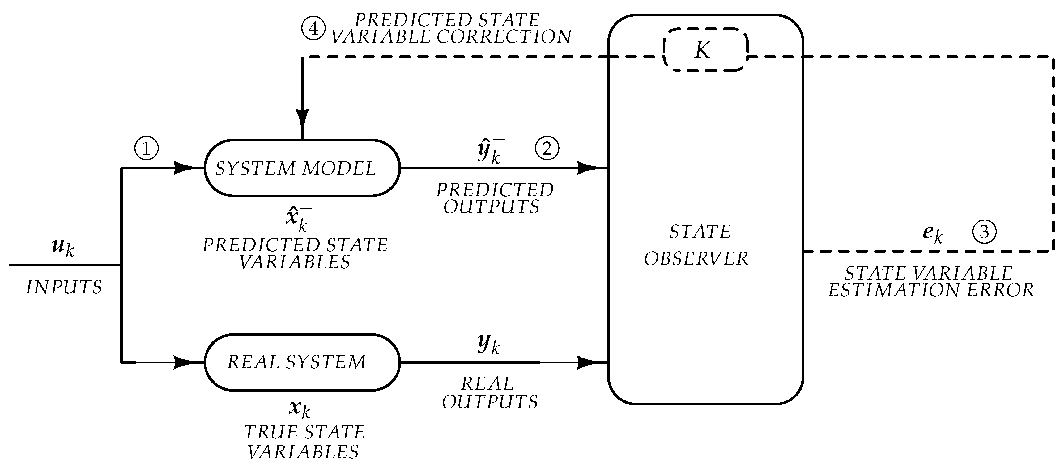
2. The Extended Kalman Filter (EKF)

2.1. The Operating Principle of the EKF

The EKF is a tool that allows to estimate the state variables of a system based on a continuous comparison at each time step of the outputs measured in the system and those predicted from its model [11,12]. The working principle of the EKF, which is depicted in Figure 1, can be described as follows. For the sake of simplicity, in this model of the EKF the process and measurement noise are considered to be additive.

To start the filter ①, an initial assumption of the state variables ${\widehat{\mathit{x}}}_{k-1}$ and of the error covariance matrix ${\mathit{P}}_{k-1}$ is required. After that, the state variable estimation process, which is made up of two phases, begins. In the first phase, known as the prediction phase, the state variable estimates ${\widehat{x}}_{k-1}$ are projected ahead for the next time step k based on the knowledge of the inputs and of the model describing the dynamics of the system. In addition, the a priori covariance matrix ${\mathit{P}}_k^{-}$ is determined. As it can be observed from (3)–(4), the update of the a priori state variable estimations and of the covariance matrix requires the knowledge of the inputs ${\mathit{u}}_k$, of the function $\mathit{f}$ (modelling the state variable dynamics over time) and of the process covariance matrix ${\mathit{Q}}_{k-1}$. In addition, the Jacobian matrix ${\mathit{A}}_k$ in (5) must be computed every time step.

$$\begin{array}{ccc}\hfill {\widehat{\mathit{x}}}_k^{-}& =& \mathit{f}\left({\widehat{\mathit{x}}}_{k-1}^{-},{\mathit{u}}_k,\mathbf{0}\right)\hfill \end{array}$$

(3)

$$\begin{array}{ccc}\hfill {\mathit{P}}_k^{-}& =& {\mathit{A}}_k{\mathit{P}}_{k-1}{\mathit{A}}_k^T+{\mathit{Q}}_{k-1}\hfill \end{array}$$

(4)

$$\begin{array}{ccc}\hfill {\mathit{A}}_k& =& \frac{\partial \mathit{f}\left({\widehat{\mathit{x}}}_{k-1}^{-},{\mathit{u}}_k,\mathbf{0}\right)}{\partial \mathit{x}}\hfill \end{array}$$

(5)

Starting from the above data, it is possible to predict the outputs of the system ${\widehat{y}}_k$ ② as follows:

$${\widehat{\mathit{y}}}_k=\mathit{g}\left({\widehat{\mathit{x}}}_k^{-},{\mathit{u}}_k,\mathbf{0}\right)$$

(6)

where $\mathit{g}$ is the function that describes the system output dynamics over time.

In the second phase of the estimation process ③, known as the correction phase, the predicted and measured outputs (${\widehat{\mathit{y}}}_k$ and ${\mathit{z}}_k$) are compared: any difference between these two outputs is interpreted by the EKF as an estimation error in the state variables, ${\mathit{e}}_k$. Besides, if the model and the real system are characterized by the same input and the model describes the system accurately enough, the difference between the measured and predicted outputs is due exclusively to a deviation of the assumed state variables with respect to their true value. The state variable estimation error is exploited by the filter to correct the state variable estimations and to compute the a posteriori covariance matrix ${\mathit{P}}_k$ ④. The computations carried out in the correction phase are the following:

$$\begin{array}{ccc}\hfill {\mathit{K}}_k& =& {\mathit{P}}_k^{-}{\mathit{H}}_k^T{\left({\mathit{H}}_k{\mathit{P}}_k^{-}{\mathit{H}}_k^T+{\mathit{R}}_k\right)}^{-1}\hfill \end{array}$$

(7)

$$\begin{array}{ccc}\hfill {\widehat{\mathit{x}}}_k& =& {\widehat{\mathit{x}}}_k^{-}+{\mathit{K}}_k\left({\mathit{z}}_k-{\widehat{\mathit{y}}}_k\right)\hfill \end{array}$$

(8)

$$\begin{array}{ccc}\hfill {\mathit{H}}_k& =& \frac{\partial \mathit{g}\left({\widehat{\mathit{x}}}_k^{-},{\mathit{u}}_k,\mathbf{0}\right)}{\partial \mathit{x}}\hfill \end{array}$$

(9)

$$\begin{array}{ccc}\hfill {\mathit{P}}_k& =& \left(\mathit{I}-{\mathit{K}}_k{\mathit{H}}_k\right){\mathit{P}}_k^{-}\hfill \end{array}$$

(10)

where ${\mathit{R}}_k$ is the noise covariance matrix, ${\mathit{K}}_k$ is the Kalman gain and ${\mathit{H}}_k$ is a matrix analogous to ${\mathit{A}}_k$. Correction and prediction phases (i.e., the phases from ② to ④) are carried out by the EKF at each time step, allowing the state variable estimates to converge eventually to their true value.

2.2. The EKF-Based Inertia Estimation Method

The EKF can be adopted to estimate in real time the inertia constant of a synchronous generator [4,5]. In this method, the state variables considered are the rotor electrical angle $\delta$, its per-unit angular speed $\omega$ and the inertia constant of the generator H (11). It is worth noting that despite not being a state variable, the inertia constant H is anyway included in the state variable vector $\mathit{x}$ to enable its estimation by means of the EKF

$$\begin{array}{cc}\hfill {\mathit{x}}_{k-1}& =\left(\begin{array}{c}{\delta }_{k-1}\\ {\omega }_{k-1}\\ H_{k-1}\end{array}\right).\hfill \end{array}$$

(11)

The state variables are updated every time step using:

$$\begin{array}{c}\hfill {\widehat{\mathit{x}}}_k^{-}=\mathit{f}\left({\widehat{\mathit{x}}}_{k-1}^{-},{\mathit{u}}_k,\mathbf{0}\right)=\left(\begin{array}{c}{\delta }_{k-1}+({\omega }_{k-1}-{\omega }_0){\omega }_B\Delta t\\ {\omega }_{k-1}+\frac{\Delta t}{2H}\left[\frac{E{V}_k}{X_{\mathrm{d}}}sin\left({\delta }_{k-1}-{\vartheta }_{k-1}\right)-D\left({\omega }_{k-1}-{\omega }_0\right)\right]\\ H_{k-1}\end{array}\right),\end{array}$$

(12)

where ${\omega }_0$ and ${\omega }_{\mathrm{B}}$ are the reference rotor angular speed in per-unit and in $\mathrm{rad}$/$\mathrm{s}$; $\Delta t$ is the filter time step; $X_{\mathrm{d}}$ and D are respectively the generator’s internal reactance and damping factor; and E is the no-load voltage of the generator. Contrary to the inertia constant, this model of the EKF assumes the internal parameters of the generators (i.e., $X_{\mathrm{d}}$ and D) to be known for the sake of simplicity. More complex EKF models, which treat such parameters as unknowns and whose equations describe the behavior of the complete model of the generator, as well as of frequency and voltage control mechanisms, can be found in [6,7,8].

The inputs used by the EKF are the generator mechanical power output $P_{\mathrm{m}}$, the voltage V and the load angle $\vartheta$ at the point of connection of the generator. The outputs predicted by the EKF and measured in the system are the active and reactive power of the synchronous generator (13). Except for $\delta$, ${\omega }_B$ and H, all the other parameters in (12)–(13) are expressed in per-unit

$$\begin{array}{cc}\hfill {\widehat{\mathit{y}}}_k^{-}& =\left(\begin{array}{c}{\widehat{P}}_k\\ {\widehat{Q}}_k\end{array}\right)=\mathit{g}\left({\widehat{\mathit{x}}}_k^{-},{\mathit{u}}_k,\mathbf{0}\right)=\left(\begin{array}{c}\frac{E{V}_{k-1}}{X_{\mathrm{d}}}sin\left({\delta }_{k-1}-{\vartheta }_{k-1}\right)\\ \frac{-V_k^2+E{V}_{k-1}cos\left({\delta }_{k-1}-{\vartheta }_{k-1}\right)}{X_{\mathrm{d}}}\end{array}\right).\hfill \end{array}$$

(13)

As it can be observed from (12), the EKF-based inertia estimation method relies on equations that describe the dynamic behavior of the simplified model of synchronous generator and neglects the presence of voltage and frequency control mechanisms. In particular, the equation used to update the rotor angular speed $\omega$ at each time step derives from the swing equation, which determines the frequency behavior of the synchronous generator right after a power disturbance (i.e., the inertial response). Therefore, to estimate the inertia, the EKF should receive measurements pertinent with an unbalancing event (e.g., a connection or disconnection of a load), since only in such case the dynamic behavior of the generator can be observed. Moreover, to operate properly, the EKF-based inertia estimation process requires to be started at about the true time of disturbance. Otherwise, the measured output may not reflect the inertial response of the generator, thereby preventing the correct estimation of the state variables.

The time of disturbance is a parameter that can only be estimated, as it cannot be known in advance. In [13], a disturbance is deemed to occur when the magnitude of the rate of change of frequency (rocof) trespasses a given threshold (e.g., $0.04\mathrm{Hz}/\mathrm{s}$). However, it is argued that a common threshold may not always be applicable to every power system, as the rocof depends on the size of the disturbance and on the characteristics of the grid (e.g., inertia constant, topology). Therefore, the time of disturbance could be inaccurately estimated. In turn, this could lead to additional errors in the inertia estimates obtained with the EKF-based method, which are investigated in Section 4.

3. The Window-Based Method for the Simultaneous Estimation of the Inertia and of the Time of Disturbance

As the EKF-based method, the window-based method is based on the swing equation [14,15]. Assuming a power imbalance occurring at given time $t_0$, the frequency dynamics immediately before and after that time instant can be described by means of (14)–(15). With respect to (1), in both equations the damping torque $D\Delta f$ has been neglected, assuming small frequency deviations right after the disturbance:

$$\begin{array}{cc}\hfill P_{\mathrm{m}}\left(t_0^{-}\right)-P_{\mathrm{e}}\left(t_0^{-}\right)& =2H\frac{\partial f\left(t_0^{-}\right)}{\partial t}\hfill \end{array}$$

(14)

$$\begin{array}{cc}\hfill P_{\mathrm{m}}\left(t_0^{+}\right)-P_{\mathrm{e}}\left(t_0^{+}\right)& =2H\frac{\partial f\left(t_0^{+}\right)}{\partial t}\hfill \end{array}$$

(15)

By subtracting (15) from (14) and recalling that the mechanical power $P_{\mathrm{m}}\left(t\right)$ cannot change instantaneously after a disturbance (i.e., $P_{\mathrm{m}}\left(t_0^{+}\right)-P_{\mathrm{m}}\left(t_0^{-}\right)=0$) one obtains

$$2H\left(\frac{\partial f\left(t_0^{+}\right)}{\partial t}-\frac{\partial f\left(t_0^{-}\right)}{\partial t}\right)=P_{\mathrm{e}}\left(t_0^{-}\right)-P_{\mathrm{e}}\left(t_0^{+}\right).$$

(16)

Thus, the inertia constant can be expressed as

$$H=\frac{1}{2}\frac{P_{\mathrm{e}}\left(t_0^{-}\right)-P_{\mathrm{e}}\left(t_0^{+}\right)}{\frac{\partial f\left(t_0^{+}\right)}{\partial t}-\frac{\partial f\left(t_0^{-}\right)}{\partial t}}=\frac{1}{2}\frac{p_1-p_2}{r_2-r_1}.$$

(17)

According to (17), the estimation of the inertia constant requires the knowledge of four values: the electrical power output of the generator and the frequency derivative (i.e., the rocof), both before and after the occurrence of the power imbalance. However, using just one measurement sample before and after the disturbing event would make the inertia estimation process extremely sensitive to the measurement noise. As a consequence, the inertia constant is instead computed starting from the parameters $p_1$, $p_2$, $r_1$ and $r_2$ (18)–(21), which consist of a measurement average over a given number of samples A (which is supposed to be the same for each of the four parameters for the sake of simplicity), both of power and rocof. In the equations, $t_{\mathrm{s}}$ is the sampling time and W is the window width of the moving average filter used for a priori measurement filtering:

$$\begin{array}{cc}\hfill p_1& =\frac{{\displaystyle \sum _{i=t_0-A{\mathrm{t}}_{\mathrm{s}}}^{t_0}}{P}_{\mathrm{e}}\left(t\right)}{A}\hfill \end{array}$$

(18)

$$\begin{array}{cc}\hfill p_2& =\frac{{\displaystyle \sum _{i=t_0+W{t}_{\mathrm{s}}}^{t_0+W\Delta t+At}}{P}_{\mathrm{e}}\left(t\right)}{A}\hfill \end{array}$$

(19)

$$\begin{array}{cc}\hfill r_1& =\frac{{\displaystyle \sum _{i=t_0-A{t}_{\mathrm{s}}}^{t_0}}\frac{\partial f\left(t\right)}{\partial t}}{A}\hfill \end{array}$$

(20)

$$\begin{array}{cc}\hfill r_2& =\frac{{\displaystyle \sum _{i=t_0+W{t}_{\mathrm{s}}}^{t_0+W{t}_{\mathrm{s}}+At}}\frac{\partial f\left(t\right)}{\partial t}}{A}\hfill \end{array}$$

(21)

In [14], the sensitivity of the window-based method to the assumed time of disturbance has been analyzed. Analogously to the EKF-based method, the inertia estimates obtained with the window-based method depend on the time at which the estimation process is started. For instance, if the time of disturbance is overestimated, the method may exploit measurements that do not describe the inertial response, as frequency adjustment mechanisms could be already activated. As a result, this introduces additional inertia estimation errors. In [16], it was noted that by executing the window-based method continuously over time, the inertia estimates showed a region of convergence at about the true time of disturbance. The estimates in such region reflected the true inertia constant of the generator: this property has been exploited to derive a method that allows a simultaneous estimation of the time of disturbance and of the inertia.

The operating principle of such a method is the following. At every time instant $t_n$ power and rocof measurements are retrieved, and the inertia constant is computed using (17). Then, the residual of N consecutive inertia estimates with respect to the current inertia estimation $H\left(t_n\right)$ is computed

$$r\left(t_n\right)=\sum _{i=t_n-N{t}_{\mathrm{s}}}^{t_n-t_{\mathrm{s}}}{(H\left(i\right)-H\left(t_n\right))}^2.$$

(22)

After that, the parameter $\mathrm{CSUM}$ is updated

$$\mathrm{CSUM}\left(t_n\right)=\left(\mathrm{CSUM}\left(t_n-t_{\mathrm{s}}\right)+1\right)C_{\mathrm{R}}{C}_{\mathrm{L}}.$$

(23)

$\mathrm{CSUM}$ is a counter that indicates how many times in a row the N consecutive inertia estimates have shown similar values. $C_{\mathrm{R}}$ and $C_{\mathrm{L}}$ are binary values: the former is set to one only if the residual at time $t_n$ is below a maximum value $r_{max}\left(t_n\right)$ defined as the product of the inertia estimate at $t_n$ and a threshold $\Theta$

$$r_{max}\left(t_n\right)=H\left(t_n\right)\Theta ;$$

(24)

the latter is equal to one only if $H\left(t_n\right)$ is greater than $\mathrm{LB}\left(t\right)$ and smaller than $\mathrm{UB}\left(t\right)$—referred to as confidence curves in [16]—

$$\begin{array}{cc}\hfill \mathrm{LB}\left(t\right)& =H_{\mathrm{p}}(1-m_{\mathrm{v}})+\left({\mathrm{LB}}_L-H_{\mathrm{p}}(1-m_{\mathrm{v}})\right)\left(1-e^{-(t-{\mathrm{t}}_{\mathrm{p}})\beta }\right)\hfill \end{array}$$

(25)

$$\begin{array}{cc}\hfill \mathrm{UB}\left(t\right)& =H_{\mathrm{p}}(1+m_{\mathrm{v}})+({\mathrm{UB}}_L-H_{\mathrm{p}}(1-m_{\mathrm{v}}))\left(1-e^{-(t-{\mathrm{t}}_{\mathrm{p}})\beta }\right)\hfill \end{array}$$

(26)

These curves represent respectively the minimum and maximum allowed values of inertia at a given time t. $H_{\mathrm{p}}$ and ${\mathrm{t}}_{\mathrm{p}}$ are the inertia and time of disturbance estimate associated with the last disturbance detected by the method; ${\mathrm{LB}}_L$ and ${\mathrm{UB}}_L$ are respectively the minimum and maximum inertia estimates expected by grid operators; $m_{\mathrm{v}}$ is the maximum expected variation in power system inertia; and $\beta$ is a parameter that describes how fast the assumed inertia constant of the grid can change after a disturbance has been detected. To tune the parameters of the confidence curves, it is necessary for grid operators to have at least partial information about the conditions of their grids. The binary values $C_{\mathrm{R}}$ and $C_{\mathrm{L}}$ have different purposes. On the one hand, $C_{\mathrm{R}}$ allows to reset $\mathrm{CSUM}$ to zero if the residue r at a given time exceeds the threshold, thereby discarding strongly varying trends of inertia estimates; on the other hand, $C_{\mathrm{L}}$ prevents false detections and allows to discard bad data due to measurement errors. A disturbance is deemed to have occurred if, over a given time interval, the inertia estimates show similar values. In particular, the algorithm detects a disturbance when $\mathrm{CSUM}$ has reached a value equal to A (i.e., the number of samples falling in a window). In such case, the assumed time of disturbance $t_{\mathrm{d}}$ is

$$t_{\mathrm{d}}=t_n-\left((2A-1)+W\right)t_{\mathrm{s}}.$$

(27)

4. Results

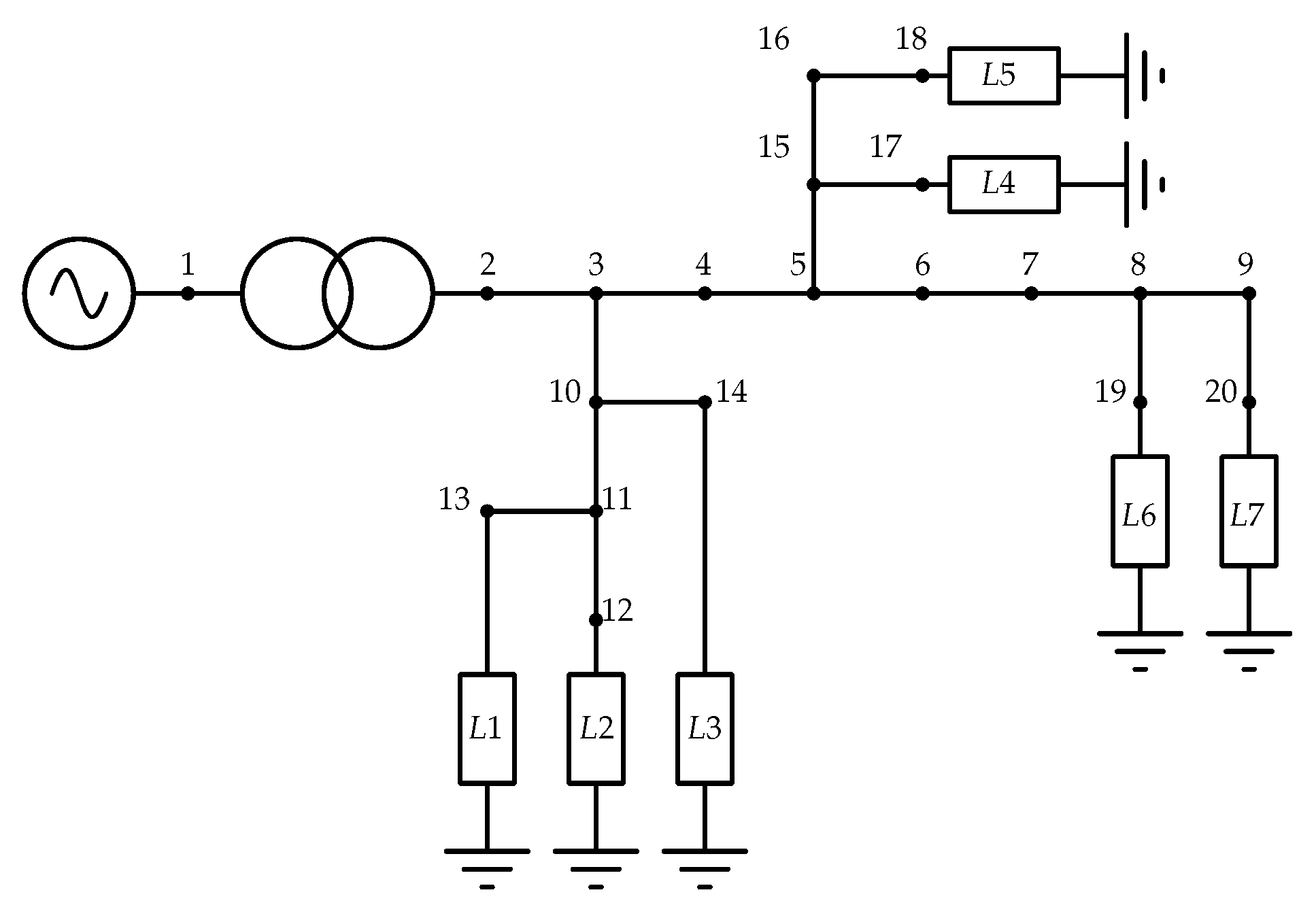
4.1. The Simulated Circuit

The EKF-based method has been adopted to estimate the inertia constant of a low voltage microgrid—whose schematic is shown in Figure 2—simulated in Simulink. With respect to [17], the external power supply has been replaced with a synchronous generator, whose inertia is $6.5$ $\mathrm{s}$. The parameters of transformer, loads, lines, and synchronous generator used in the simulations are reported in

Table A1. Characteristics of the MV/LV transformer (nodes 1–2).

Connection		3-ph $\mathbf{\Delta }$-Y Grounded
$S_{\mathrm{n}}$	$\mathrm{k}\mathrm{VA}$	300
$V_{1_{\mathrm{n}}}$	$\mathrm{k}\mathrm{V}$	20
$V_{2_{\mathrm{n}}}$	$\mathrm{k}\mathrm{V}$	0.4
$X_{\mathrm{tr}}$	$\mathrm{p}.\mathrm{u}.$	0.032

,

Table A2. Characteristics of the loads.

Load	Rated Power kVA	Power Factor
L1	30	0.85
L2	8	0.85
L3	25	0.85
L4	16	0.85
L5	8	0.85
L6	25	0.85
L7	20	0.85

,

Table A3. Characteristics of the lines.

From Node	To Node	${\mathit{R}}_{\mathbf{ph}}$ Ω/km	${\mathit{X}}_{\mathbf{ph}}$ Ω/km	${\mathit{R}}_{\mathbf{o}}$ Ω/km	${\mathit{X}}_{\mathbf{o}}$ Ω/km	L m
1	2	0.387	0.295	0.619	0.472	30
2	3	0.387	0.295	0.619	0.472	30
3	4	0.387	0.295	0.619	0.472	30
4	5	0.387	0.295	0.619	0.472	30
5	6	0.524	0.307	0.838	0.491	30
6	7	0.524	0.307	0.838	0.491	30
7	8	0.524	0.307	0.838	0.491	30
8	9	0.524	0.307	0.838	0.491	30
3	10	0.524	0.307	0.838	0.491	30
10	11	1.150	0.332	0.838	0.491	30
11	12	1.150	0.332	1.840	0.531	30
11	13	1.150	0.332	1.840	0.531	30
10	14	1.150	0.332	1.840	0.531	30
5	15	1.150	0.332	1.840	0.531	30
15	16	1.150	0.332	1.840	0.531	30
15	17	1.150	0.332	1.840	0.531	30
16	18	1.150	0.332	1.840	0.531	30
8	19	1.150	0.332	1.840	0.531	30
9	20	1.150	0.332	1.840	0.531	30

,

Table A4. Characteristics of the synchronous generator.

Pole pairs		2
$S_{\mathrm{n}}$	$\mathrm{M}\mathrm{VA}$	1
$V_{\mathrm{n}}$	$\mathrm{k}\mathrm{V}$	20
$f_{\mathrm{n}}$	$\mathrm{Hz}$	50
H	$\mathrm{s}$	6.5
D	$\mathrm{p}.\mathrm{u}.$	0
$R_{\mathrm{s}}$	$\mathrm{p}.\mathrm{u}.$	0.0025
$X_{\mathrm{d}}$	$\mathrm{p}.\mathrm{u}.$	1.8
$X_{\mathrm{d}}^{{}^{\prime }}$	$\mathrm{p}.\mathrm{u}.$	0.3
$X_{\mathrm{d}}^{{}^{″}}$	$\mathrm{p}.\mathrm{u}.$	0.25
$X_{\mathrm{q}}$	$\mathrm{p}.\mathrm{u}.$	1.7
$X_{\mathrm{q}}^{{}^{\prime }}$	$\mathrm{p}.\mathrm{u}.$	0.55
$X_{\mathrm{q}}^{{}^{″}}$	$\mathrm{p}.\mathrm{u}.$	0.25
$X_{\mathrm{l}}$	$\mathrm{p}.\mathrm{u}.$	0.2
$T_{\mathrm{d}0}^{{}^{\prime }}$	$\mathrm{s}$	8.0
$T_{\mathrm{d}0}^{{}^{″}}$	$\mathrm{s}$	0.03
$T_{\mathrm{q}0}^{{}^{\prime }}$	$\mathrm{s}$	0.4
$T_{\mathrm{q}0}^{{}^{″}}$	$\mathrm{s}$	0.05

in the Appendix A. Simulations were executed for 8 $\mathrm{s}$, with a sampling time of $0.1$ $\mathrm{m}$$\mathrm{s}$. The power unbalancing event—exploited by the EKF to estimate the inertia of the synchronous generator—occurred at 3 $\mathrm{s}$ and consisted in the disconnection of the load L7 (whose active power withdrawal is $21.25$ $\mathrm{k}$$\mathrm{W}$), as well as of the line between the nodes 9 and 20.

Different scenarios (shown in

Table 1. Scenarios analyzed during the simulations.

Case ID	Generator Model	Primary Frequency Regulation Activation
A	Simplified	✘
B	Simplified	✔ ($\tau =1\mathrm{s}$, $K=10\mathrm{p}.\mathrm{u}.$)
C	Simplified	✔ ($\tau =2\mathrm{s}$, $K=10\mathrm{p}.\mathrm{u}.$)
D	Complete	✘
E	Complete	✔ ($\tau =1\mathrm{s}$, $K=10\mathrm{p}.\mathrm{u}.$)
F	Complete	✔ ($\tau =2\mathrm{s}$, $K=10\mathrm{p}.\mathrm{u}.$)

) were simulated, assuming, for the same disturbing event, the presence (or the absence) of primary frequency regulation and the adoption of a complete (or simplified) model of the synchronous generator. Cases B and C (as well as E and F) are aimed at analyzing the influence of a slower and faster frequency control in the inertia estimation process. The primary frequency control block scheme used by the governor is depicted in Figure 3. The parameter K, known as droop constant, is linked to the steady-state value of the frequency f at the end of primary frequency regulation: the higher K, the lower f at steady-state. On the contrary, the parameter $\tau$ is linked to the time needed by the frequency transient owed to primary regulation to reach completion. Consider for instance Figure 4, which depicts two frequency transients related with the same power disturbance occurring at 3 $\mathrm{s}$. The blue and red curves are associated with the values of $\tau$ and K used in the cases B and C (and E and F) shown in Table 1. It can be observed that the two curves share the same steady-state frequency, as their value of K is identical. However, since the red curve has a higher $\tau$, it requires more time to reach the steady-state value with respect to the blue curve.

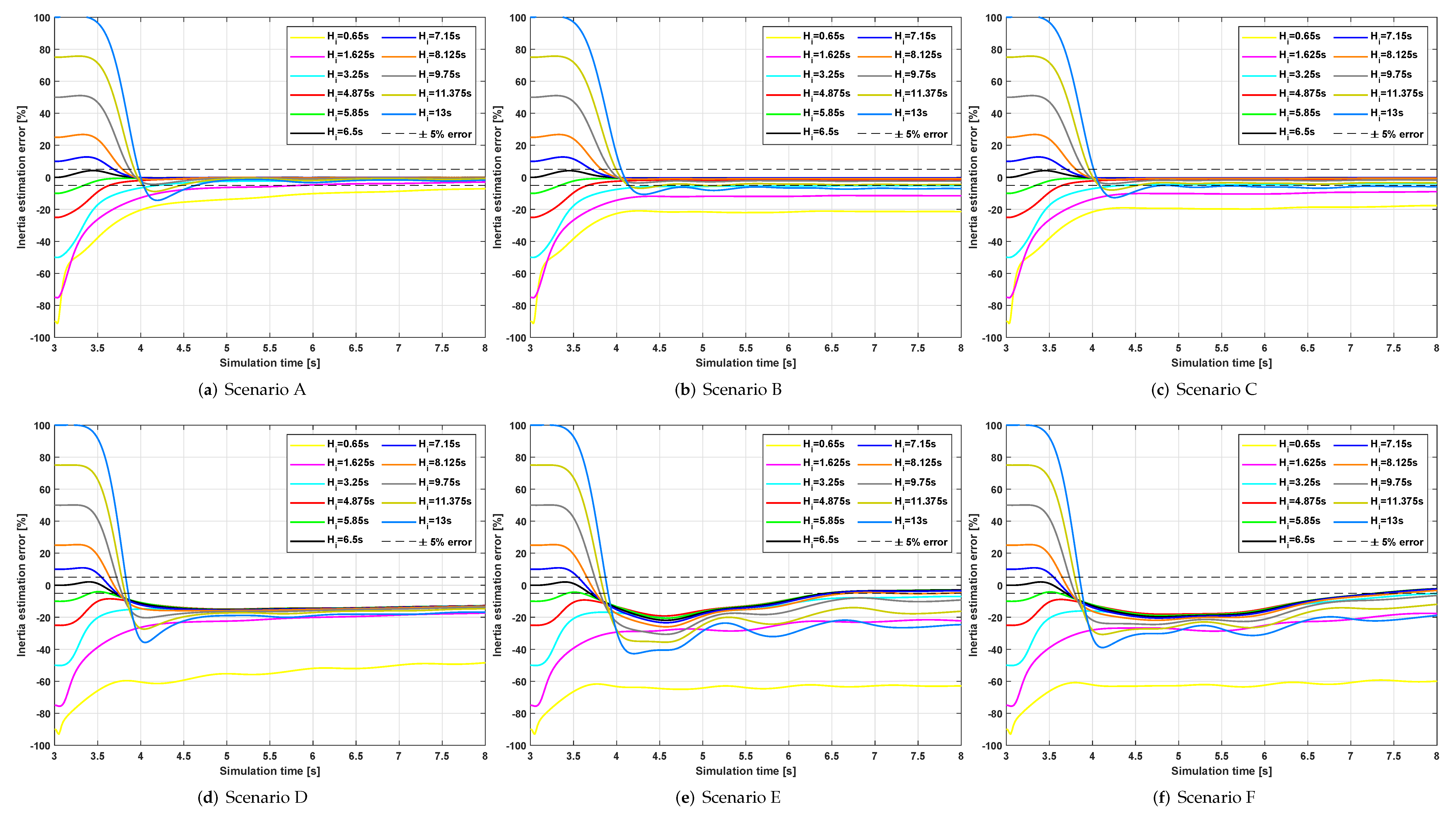
4.2. Analysis of the Sensitivity of EKF-Based Inertia Estimation Method to the Assumed Time of Disturbance

The EKF-based inertia estimation method has been adopted to estimate the inertia of the synchronous generator in Figure 2 for every scenario shown in Table 1. At first, the EKF has been started at the true time of disturbance (i.e., 3 $\mathrm{s}$), which was supposed to be known (such hypothesis is removed later in the paper). The filter time step has been set to $0.1$ $\mathrm{m}$$\mathrm{s}$: such a low time step, although incompatible with modern measurement systems, can be obtained by means of data interpolation. To begin the estimation process, an initial assumption of the state variables (11) is necessary: ${\delta }_{k-1}$ and ${\omega }_{k-1}$ have been set respectively to 0 $\mathrm{rad}$ and 1 $\mathrm{p}.\mathrm{u}.$; for what concerns the initially assumed inertia constant $H_{k-1}$, the EKF has been started with 11 different values, associated with an initial estimation error ranging between $-90\%$ and $100\%$. Moreover, the diagonal elements of the error covariance matrix $P_{k-1}$ (a 3-by-3 matrix) have been set to 2 $\mathrm{rad}$, $0.001$ $\mathrm{p}.\mathrm{u}.$ and 10 $\mathrm{s}$. The inertia estimates obtained for each case are depicted in Figure 5. The x and y axes of each plot are respectively the simulation time (in $\mathrm{s}$) and the inertia estimation error (expressed as a percentage). Each colored curve refers to a specific initial inertia estimate used to start the filter.

To begin with, consider Figure 5a–c, which refer to scenarios A, B, and C, where the simplified model of the synchronous generator is adopted. The differences in estimation errors in the plots are due to the absence or the presence of a slower or faster primary frequency regulation, based on the scenario considered. Within 4 $\mathrm{s}$ of simulation time (i.e., 1 $\mathrm{s}$ of use time of the EKF), the inertia estimation error converges inside the $\pm 5\%$ band for most curves. It can be noticed that the higher the module of the initial inertia estimation error, the longer it takes for the EKF to converge to a final estimate and, thus, a final error. In fact, the filter requires more prediction and correction phases to compensate the high initial errors and bring the assumed state variable vector closer to the true one. Therefore, if the initial inertia estimation error is too high, the EKF may be unable to provide a correct inertia estimate in a short time. For example, this is what happens in Figure 5b to the yellow curve (corresponding to an initial inertia estimate of $H_{k-1}=0.65\mathrm{s}$ and an initial error of $-90\%$), whose estimation error amounts to about $-20\%$ even after using the EKF for 5 $\mathrm{s}$. However, such a high initial error may be reputed unrealistic, as grid operators are expected to have at least partial information about the inertia of the generators connected to their grids.

Consider now Figure 5d–f. In this case, a general decrease in estimation accuracy can be observed, as the estimation error never lies in the $\pm 5\%$ band, regardless of the initially assumed inertia constant. For instance, if the EKF is used for 1 $\mathrm{s}$ starting from the time of disturbance, the inertia estimation error amounts to $-13\%$ at best. The reason for this decrease in accuracy is due to the fact that in the EKF model presented in this paper, the equations used to update the state variables (12) describe the simplified behavior of the synchronous generator, which consists of a voltage source in series with a synchronous reactance and resistance. Such model neglects all the other self- and magnetizing inductances of the armature, damping, and field windings, which, on the contrary, are considered in the complete model (simulated in case D, E, and F). As a result, (12) describes only approximately the dynamic behavior of the complete model of the synchronous generator. Therefore, using this model of the EKF-based method to estimate the inertia of the complete model of the generator leads to less accurate inertia estimates with respect to the ones obtained with the simplified model of the generator.

The above results have been obtained by starting the EKF at the true time of disturbance, which was supposed to be known. However, this hypothesis does not hold true in reality, as the time of disturbance cannot be known in advance, but it can only be estimated. As already mentioned, the time of disturbance could be determined by examining when the rocof trespasses a given threshold. Consider for instance Figure 6a,b. The former figure compares the true rocof and the rocof obtained by filtering the noisy frequency measurements of case B. In this case, frequency measurements have been down-sampled to $0.01$ $\mathrm{s}$ and a frequency noise with zero mean and a standard deviation of $5\times {10}^{-6}$ $\mathrm{p}.\mathrm{u}.$ has been added; to filter the measurement noise, a 10-sample moving average window was adopted. On the contrary, the latter figure shows how the assumed time of disturbance changes based on the rocof threshold adopted. Please note that if the rocof threshold is always higher than the filtered rocof, the time of disturbance estimate is set to 8 $\mathrm{s}$ (i.e., the simulation time). It can be observed that unless grid operators know in advance a range of rocof values that the system may take, the rocof-threshold-trespassing criterion may lead to inaccurate time of disturbance estimates.

Consequently, based on the threshold chosen, the EKF-based estimation process may be started at an assumed time of disturbance different from the true one. In turn, this could lead to additional inertia estimation errors. To prove this statement, the EKF-based inertia estimation method has been used once again. With respect to the previous simulations, the EKF has been used for a time $t_{\mathrm{dur}}$ equal to 1 $\mathrm{s}$ or 2 $\mathrm{s}$, starting from an assumed time of disturbance ranging between 2 and 4 $\mathrm{s}$ (3 $\mathrm{s}$ being the true time of disturbance). The filter time step, the initially assumed state variables and the $P_{k-1}$ matrix remained unaltered. The inertia estimates obtained for $t_{\mathrm{dur}}=1\mathrm{s}$ and $t_{\mathrm{dur}}=2\mathrm{s}$ are depicted respectively in Figure 7 and Figure 8. The x and y axes of each plot are respectively the assumed time of disturbance (in $\mathrm{s}$) and the inertia estimation error (expressed as a percentage).

To begin with, consider Figure 7a,d, which refer respectively to scenarios A and D when $t_{\mathrm{dur}}=1\mathrm{s}$. It can be observed that if primary frequency regulation is not activated, the EKF-based method is more susceptible to time of disturbance underestimation than overestimation. As a matter of fact, if the assumed time of disturbance $\widehat{t}$ is higher than the true time of disturbance $t_0$ (i.e., 3 $\mathrm{s}$), the estimates vary slightly with $\widehat{t}$, except for the curves associated with a high initial inertia estimation error (e.g., the yellow curve). On the contrary, if $\widehat{t}$ is lower than $t_0$, the estimates change noticeably with $\widehat{t}$. The reason for this biased susceptibility can be explained as follows. To operate properly, the EKF needs to receive measurements pertinent with the inertial response of the generator. A time of disturbance underestimation implies that some measurement samples that are also prior to the disturbance are adopted. However, such samples do not contribute to an improvement in the state variable estimation, as they do not reflect the dynamics of the generator right after a power imbalance. In particular, the more severe the time of disturbance underestimation, the higher the inertia estimation error, because the number of post-disturbance samples (the only ones allowing an improvement in the inertia estimations) used by the filter decreases. On the contrary, if the time of disturbance is overestimated, the inertia estimation error is slightly affected. Besides, if frequency control is absent, any sample after $t_0$ describes the inertial response of the generator and thereby contributes in improving the inertia estimates.

Consider now Figure 7b,c. The figures refer to scenarios B and C, which contemplate respectively the presence of a faster and slower primary frequency regulation. In this case, it is no longer true that if $\widehat{t}$ is higher than $t_0$ the inertia estimates change slightly with $\widehat{t}$. In fact, the higher the initial inertia estimation error, the higher the increase in the final estimation error with $\widehat{t}$. This happens because if $\widehat{t}$ is overestimated, the filter receives less measurements pertinent with the inertial response (the ones contributing primarily to a correct inertia estimation) and more measurements linked to a time period where frequency adjustment mechanisms are already activated. Those measurements contribute less to the inertia calibration process because, even though they describe the dynamic behavior of the generator to an extent, they are not linked to the inertial response. Moreover, it is worth pointing out that in case of time of disturbance overestimation, the inertia estimations of scenarios B and C are different. In fact, the estimates change more with $\widehat{t}$ in Figure 7b than in Figure 7c. The reason for such difference can be understood by analyzing the inset of Figure 4, which depicts the frequency behavior immediately after the disturbance for the blue and red curves, characterized respectively by a faster ($\tau =1\mathrm{s}$) and slower ($\tau =2\mathrm{s}$) frequency control. The dashed line describes the linear frequency behavior obtained if no control mechanisms are activated (i.e., the inertial response). It can be observed that the blue curve (scenario B) ceases to increase linearly before the red curve (scenario C), because in case B the frequency control is faster. Consequently, scenario B is characterized by less measurements related to the inertial response and, thus, is more prone to higher estimation errors if $\widehat{t}$ is overestimated. For what concerns time of disturbance underestimation, it can be noted that the inertia estimates in Figure 7b,c differ with respect to the ones in Figure 7a for $\widehat{t}$ lower than $t_0$. This is because even when $\widehat{t}$ is underestimated, the use time $t_{\mathrm{dur}}$ is such that some measurements pertinent with primary frequency regulation are included, which are absent in case A. An analogous reasoning holds for Figure 7e,f. In this case, however, not only are the inertia estimates of cases E and F inaccurate, but they also change considerably with the time of disturbance, even when the EKF is started with an initial inertia estimate close to the true one.

When the use time of the EKF $t_{\mathrm{dur}}$ is increased to 2 $\mathrm{s}$ (Figure 8), the inertia estimates of every scenario improve both in terms of accuracy and sensitivity to the assumed time of disturbance. Besides, an increased $t_{\mathrm{dur}}$ implies more prediction and correction phases by means of which the state variable estimates can be improved. This statement holds even in the scenarios where primary frequency control is considered, because also the measurements after the inertial response describe to an extent the dynamic behavior of the generator and can contribute to the inertia estimation process, although in a less significant manner with respect to the samples exclusively linked to the inertial response.

From the comparison of Figure 7 and Figure 8 it can be understood that the higher $t_{\mathrm{dur}}$, the more accurate the estimates. However, increasing the use time of the filter makes the method more demanding in terms of number of measurement samples and less practical for real-time operation purposes. This problem could be solved by carrying out several EKF estimation processes in cascade instead of a single, longer one. In this article, a high number of measurement samples is adopted to perform enough correction phases of the EKF (and, thus, bring the inertia estimations closer to their true value). On the contrary, with this solution, rather than using a high amount of measurement samples, the number of prediction and correction phases is increased by repeating the whole EKF-based calibration process several times, until the estimations converge. In every iteration, the initial inertia estimate is the last a posteriori inertia estimate obtained from the previous iteration, while the set of input and output measurements exploited is the same, as the time frame considered for the simulations does not change. By doing so, as proven in [4], the inertia estimates can still reach convergence even though the number of measurement samples adopted is reduced. In particular, the higher the number of iterations carried out, the more likely the inertia estimations to converge.

As a last comment, to make a comparison between the two inertia estimation methods presented in this paper, the window-based method has been exploited to estimate the time of disturbance and the inertia of the simulated grid for each scenario shown in Table 1. Such method has been used continuously from the beginning of the simulations. The sampling time $t_{\mathrm{s}}$ has been changed to $0.01$ $\mathrm{s}$. One thousand random noise profiles with a zero mean and a standard deviation of $5\times {10}^{-6}$ $\mathrm{p}.\mathrm{u}.$ and $5\times {10}^{-4}$ $\mathrm{p}.\mathrm{u}.$ have been added respectively to frequency and power measurements. The base frequency amounts to 50 $\mathrm{Hz}$ and the base power is 1 $\mathrm{M}$$\mathrm{VA}$. The measurements have been filtered using a moving average window of a width W of 10 samples. The parameters used in the Equations (22)–(27) are shown in

Table 2. Parameters used in the window-based method.

A	samples	30
N	samples	3
$\Theta$	—	0.5
${\mathrm{UB}}_L$	$\mathrm{s}$	13
${\mathrm{LB}}_L$	$\mathrm{s}$	0
$m_{\mathrm{v}}$	—	0.2
$\beta$	1/$\mathrm{s}$	0.01

.

The estimation results obtained with each noise profile are shown in Figure 9. It can be noted that by considering every scenario, the maximum and minimum inertia estimates are $7.1$ $\mathrm{s}$ and $6.1$ $\mathrm{s}$ (i.e., an error of $+9.23\%$ and $-6.15\%$ respectively). The maximum and minimum time of disturbance estimates are $3.04$ $\mathrm{s}$ and $2.86$ $\mathrm{s}$ (i.e., an error of $+1.33\%$ and $-4.67\%$ respectively). As a result, provided that grid operators have enough information about their grids to build reasonable confidence curves $\mathrm{UB}\left(t\right)$ and $\mathrm{LB}\left(t\right)$, the window-based method allows to correctly estimate the inertia constant and the time of disturbance and to avoid false detections.

On the one hand, the window-based method is conceptually simple and requires few measurements to provide an estimation of the inertia. The most critical issue of the method is given by the frequency noise, which, if not filtered out correctly, could result in computation errors in the rocof, and, in turn, in additional inertia estimation errors [15]. On the other hand, the EKF-based method is more complex and requires more measurements but it allows also the simultaneous estimation of other parameters than inertia.

5. Conclusions

In this paper, the sensitivity of the EKF-based inertia estimation method to the assumed time of disturbance is analyzed. Simulation results show that such sensitivity is influenced by the initially assumed inertia constant, the use time of the filter and the time required for primary frequency regulation to be activated. In particular, the following conclusions can be drawn:

• The number of prediction and correction phases required to bring the final inertia estimate to convergence increases with the magnitude of the initial inertia estimation error. Therefore, depending on the use time of the filter and on the initially assumed inertia constant, the final inertia estimation error could still be too high, as the inertia estimate has not yet reached convergence. Moreover, the estimation process strongly benefits from the measurement samples pertaining to the inertial response of the synchronous generator. Considering a fixed use time of the filter, a wrong time of disturbance estimation implies that less measurements belonging to that phase may be used. In turn, this decreases the estimation accuracy of the EKF and worsens the final inertia estimate in case of high initial estimation errors, as well. To sum up, the higher the initial inertia constant estimation error used to start the filter, the higher the estimation errors and the sensitivity of the method to the assumed time of disturbance.
• The use time of the filter has an overall beneficial effect on the inertia estimates, both in terms of accuracy and of sensitivity to the assumed time of disturbance.
• In general, the method is more sensitive to time of disturbance underestimation than overestimation. In particular, when primary frequency regulation is absent, such sensitivity reduces as the use time of the filter increases. On the contrary, if primary frequency regulation is activated, the faster such control, the higher the inertia estimation error in case of time of disturbance overestimation.

Future research will be devoted to analyze a new model of an EKF-based method whose equations describe more accurately the behavior of the complete model of the synchronous generator, as well as of other equipment (such as frequency and voltage regulation systems). This would improve the inertia estimation process, both in terms of accuracy and sensitivity to a wrong assumed time of disturbance.

References

1. Ørum, E.; Kuivaniemi, M.; Laasonen, M.; Bruseth, A.I.; Jansson, E.A.; Danell, A.; Elkington, K.; Modig, N. Future System Inertia; Technical Report; ENTSOE: Brussels, Belgium, 2015. [Google Scholar]
2. Tielens, P.; Van Hertem, D. The relevance of inertia in power systems. Renew. Sustain. Energy Rev. 2016, 55, 999–1009. [Google Scholar] [CrossRef] [Green Version]
3. Tamrakar, U.; Shrestha, D.; Maharjan, M.; Bhattarai, B.P.; Hansen, T.M.; Tonkoski, R. Virtual Inertia: Current Trends and Future Directions. Appl. Sci. 2017, 7, 654. [Google Scholar] [CrossRef]
4. Huang, Z.; Du, P.; Kosterev, D.; Yang, B. Application of Extended Kalman Filter Techniques for Dynamic Model Parameter Calibration. In Proceedings of the IEEE Power and Energy Society General Meeting, Calgary, AB, Canada, 26–30 July 2009; pp. 1–8. [Google Scholar]
5. Kalsi, K.; Sun, Y.; Huang, Z.; Du, P.; Diao, R.; Anderson, K.K.; Li, Y.; Lee, B. Calibrating Multi-machine Power System Parameters with the Extended Kalman Filter. In Proceedings of the IEEE Power and Energy Society General Meeting, Detroit, MI, USA, 24–28 July 2011; pp. 1–8. [Google Scholar]
6. Huang, Z.; Du, P.; Kosterev, D.; Yang, S. Generator Dynamic Model Validation and Parameter Calibration Using Phasor Measurements at the Point of Connection. IEEE Trans. Power Syst. 2013, 28, 1939–1949. [Google Scholar] [CrossRef]
7. Aghamolki, H.G.; Miao, Z.; Fan, L.; Jiang, W.; Manjure, D. Identification of synchronous generator model with frequency control using unscented Kalman filter. Electr. Power Syst. Res. 2015, 126, 45–55. [Google Scholar] [CrossRef] [Green Version]
8. Zhou, N.; Meng, D.; Huang, Z.; Welch, G. Dynamic State Estimation of a Synchronous Machine Using PMU Data: A Comparative Study. IEEE Trans. Smart Grid 2015, 6, 450–460. [Google Scholar] [CrossRef]
9. Ariff, M.A.M.; Pal, B.C.; Singh, A.K. Estimating Dynamic Model Parameters for Adaptive Protection and Control in Power System. IEEE Trans. Power Syst. 2015, 30, 829–839. [Google Scholar] [CrossRef] [Green Version]
10. Fan, L.; Wehbe, Y. Extended Kalman filtering based real-time dynamic state and parameter estimation using PMU data. Electr. Power Syst. Res. 2013, 103, 168–177. [Google Scholar] [CrossRef]
11. Rhodes, I.B. A Tutorial Introduction to Estimation and Filtering. IEEE Trans. Autom. Control 1971, 16, 688–706. [Google Scholar] [CrossRef]
12. Welch, G.; Bishop, G. An Introduction to the Kalman Filter; Technical Report TR 95-041; University of North Carolina: Chapel Hill, NC, USA, 2006. [Google Scholar]
13. Inoue, T.; Taniguchi, H.; Ikeguchi, Y.; Yoshida, K. Estimation of Power System Inertia Constant and Capacity of Spinning-reserve Support Generators Using Measured Frequency Transients. IEEE Trans. Power Syst. 1997, 12, 136–143. [Google Scholar] [CrossRef]
14. Wall, P.; Gonzalez-Longatt, F.; Terzija, V. Estimation of generator inertia available during a disturbance. In Proceedings of the IEEE Power and Energy Society General Meeting, San Diego, CA, USA, 22–26 July 2012; pp. 1–8. [Google Scholar]
15. Wall, P.; Regulski, P.; Rusidovic, Z.; Terzija, V. Inertia estimation using PMUs in a Laboratory. In Proceedings of the IEEE PES Innovative Smart Grid Technologies Conference Europe, Washington, DC, USA, 17–20 February 2015; pp. 1–6. [Google Scholar]
16. Wall, P.; Terzija, V. Simultaneous Estimation of the Time of Disturbance and Inertia in Power Systems. IEEE Trans. Power Deliv. 2014, 29, 2018–2031. [Google Scholar] [CrossRef]
17. Strunz, K. Benchmark Systems for Network Integration of Renewable and Distributed Energy Resources; Technical Report 575, CIGRÉ TF C6.04.02; CIGRÉ: Paris, France, 2014. [Google Scholar]
Figure 1. The operating principle of the EKF.
Energies 12 00483 g001
Figure 2. Schematic of the circuit used for the validation of the EKF-based method [17]. The segments between each couple of nodes correspond to r-l lines, whose parameters are specified in the Appendix A.
Energies 12 00483 g002
Figure 3. The primary frequency control scheme used during the simulations. P m and f are the mechanical power output and the frequency of the generator. The subscript n denotes the nominal value.
Energies 12 00483 g003
Figure 4. Comparison between two frequency transients.
Energies 12 00483 g004
Figure 5. EKF-based inertia estimates, obtained by starting the EKF at the true time of disturbance.
Energies 12 00483 g005
Figure 6. Comparison between true and filtered rocof for case B (a); time of disturbance estimation by means of rocof trespassing criterion (b).
Energies 12 00483 g006
Figure 7. Analysis of the EKF-based inertia estimates to the assumed time of disturbance (tdur = 1 s). The colored curves in each plot refer to the same legend. For the sake of clarity, the legend is only included in the plots where it does not overlap with the curves.
Energies 12 00483 g007
Figure 8. Analysis of the EKF-based inertia estimates to the assumed time of disturbance (tdur = 2 s). The colored curves in each plot refer to the same legend. For the sake of clarity, the legend is only included in the plots where it does not overlap with the curves.
Energies 12 00483 g008
Figure 9. Inertia and time of disturbance estimates obtained with the window-based method. The blue dots are the estimates obtained for each noise profile considered. The red dot in each plot represents the true inertia and time of disturbance.
Energies 12 00483 g009