Consensus-Based Method for Anomaly Detection in VAV Units

Abstract

Buildings account for large part of global energy consumption. Besides energy consumed due to normal operation, a large amount of energy can be wasted due to faults in buildings subsystems. Fault detection and diagnostics techniques aim to identify faults and prevent energy waste, but are often difficult to apply in practice. Data-driven methods, in particular, require an adequate amount of fault-free training data, which is rarely available. In this paper, we propose a method for anomaly detection that exploits consensus among multiple identical components. Even if some of the components are faulty, their aggregate behaviour is overall correct, and it can be used to train a data-driven model. We test our method on variable-air-volume units in an existing building, executing two experiments grouping the components according to ventilation unit, and according to room type. The two experiments identified the same set of anomalous components, i.e., their behaviour was different from the rest of the group in both cases, and this suggests that the anomaly was not due to wrong group assignment. The proposed method shows the potential of exploiting consensus among multiple identical systems to detect anomalous ones.

1. Introduction

Nowadays, buildings have a large impact on both energy consumption and other environmental effects such as carbon emissions. In the European Union they are responsible for 40% of the total energy usage and 36% of CO₂ emissions [1,2]. Similarly, in the United States, they are responsible for about 41% of primary energy consumption in 2010, which was 44% more than transports and 36% more than industry. Total building primary energy consumption in 2009 was about 48% higher than in 1980, going from 1290 TWh to 2784 TWh [3]. It is, therefore, evident that buildings are a key sector for achieving environment and climate targets such as 20 20 by 2020, i.e., 20% reduction in greenhouse gases and 20% share of renewable energy sources by year 2020 [4], and the more recent 30% energy efficiency by year 2030 [5].

Modern commercial buildings contain large and complex systems, such as heating, ventilation and air-conditioning (HVAC) and lighting, and their operation is controlled by automated building management systems (BMSs), which often require a network of sensors, meters and actuators. Faults in these systems impact building operations, e.g., by causing occupants discomfort, but also increase energy usage. The most common faults in commercial buildings in U. S. are estimated to have caused over 3.3 billion dollars in energy waste in 2009 [6], and over 7 billion dollars in 2017 [7]. It is often difficult to precisely identify faults, and sometimes even to detect them, and a system could operate for a long time before the building management even notices it is not working correctly [8]. Fault detection and diagnostics (FDD) techniques aim to detect faults and identify their precise location and cause. Research and application of FDD techniques, applied successfully in other fields for several decades, gained traction in the buildings sector in the past few years.

Ventilation units are among the largest and most critical systems in buildings, and account for large energy consumption. Their faults, such as incorrect HVAC on/off modes or inappropriate setpoints for thermostats, are responsible for a large share of energy waste [7]. While many FDD techniques have been applied to the large air handling unit (AHU), faults and misconfigurations involving variable air volume (VAV) units at room level are often ignored [9]. However, considering that the VAV units have the main responsibility of direct air supply to each room, and taking into account the importance of attaining good indoor air quality and thermal comfort, proper monitoring and FDD investigations of VAV units seems very sensible.

Many FDD techniques have major limitations when applied in practice, due to non-ideal conditions of the real world. Model-based techniques require detailed knowledge of the system under test, which is often not available. Data-driven techniques, on the other hand, require validated and fault-free historical data to learn the correct behaviour of the system. Historical data is often available, but it is rarely validated, and there is a risk that faulty behaviour is used in the training phase.

Peer validation and consensus-based validation, on the other hand, can be used to mitigate this issue. Multiple identical or similar systems are considered together, under the assumption that the majority of them operate correctly. When their historical data is used to train a model, the contributions from faulty systems are small compared with the ones from healthy ones, and their effect on the model is diluted. Therefore, the requirement for fault-free training data is lifted, and faulty systems are identified as outliers among the healthy ones. This eliminates the need for complex and sophisticated models and large system operation datasets.

The rest of the paper is organized as follows. The state of the art is reviewed in Section 2. The proposed technique is introduced in Section 3. Section 4 presents the case study and discusses results and implications. Finally, conclusions are drawn in Section 5.

2. State-of-the-Art

Kim and Katipamula present a comprehensive review of recent FDD methods for building systems [10]. The authors identify three main categories, depending on the approach used: model-based methods, data-driven methods and rules-based methods.

In model-based methods, an explicit model of the system under test is created, using first principles physics, physics and other system and envelope modelling techniques. Results obtained from the model are compared with the ones obtained from the actual system, and, if the two deviate, a fault is detected. Model-based methods have usually high accuracy and can detect faults with smaller impacts, as well as faults absent from historical data. By modifying the model, it is possible to simulate faulty conditions, which makes possible to precisely diagnose faults. On the other hand, such models require extensive knowledge of the system under test and cannot easily be extended to other systems. Correctly estimating the model’s parameters is also a challenge [11].

In data-driven–or history-based–methods, a model of the system under test is created from historical data. Several techniques exist, such as artificial neural networks, principal component analysis and statistical machine learning algorithms. The model is treated as a black box and no understanding of the system is necessary. For this reason, these methods can often be easily extended to other systems by simply re-training the model from different data. On the other hand, a relatively large amount of fault-free historical data must be available to train the model. This makes data-driven methods unsuitable for newly deployed systems and for situations where historical data is not provably fault-free. Independent sets of labeled faulty data are often necessary to perform precise fault diagnostics and identification.

In rules-based methods, a set of rules describing the behaviour of the system under test is defined. Rules are usually obtained from expert knowledge and technical documentation, and can describe both correct and faulty behaviour, which makes possible to precisely diagnose faults. No training data is necessary, and only a high-level knowledge of the system is needed. However, rules can only represent relatively simple systems and cannot properly describe complex interactions.

To the best of our knowledge, no previous work has been done on using consensus-based techniques for FDD in buildings systems, and specifically on VAV units used to control CO₂ level. Narayanaswamy et al. present a model, cluster and compare method for FDD on VAV units, where data from several units are used to detect anomalies [9]. Linear models are trained for each individual VAV unit, and the obtained parameters undergo a clustering procedure. Units that do not belong to any cluster are identified as anomalous and, finally, the results are used to generate a set of expert rules for anomaly detection. The authors deploy and test their method on a real building, and use it to detect anomalies with respect to temperature control in rooms.

Consensus techniques have been used in the field for other purposes, such as features selection. Partially redundant measurements in complex systems such as HVAC systems can make it difficult to apply FDD methods, which are often not designed to handle conflicting inputs or large amounts of inputs. Yuwono et al. present a method for feature selection using swarm intelligence and consensus clustering, which can be used to reduce and aggregate the number of features used in FDD methods [12]. Consensus clustering has the advantage that the number of clusters is not fixed in advance, instead, clusters are identified automatically.

Consensus-based techniques have also been used for FDD in other fields. FDD methods often use data and findings from models and laboratory tests to validate or predict data for systems in the field. Differences from the model, and different conditions between tests and the real world, can reduce methods accuracy and effectiveness. Byttner et al. present a FDD method for vehicles based on consensus between such models and tests, and on-field systems [13]. Data is first preprocessed on-vehicle and interesting features are identified, which are sent to a central server that collects them for all vehicles. The central server searches for outliers, i.e., features from a single vehicle that do not match the overall distribution across the entire fleet, laboratory tests, or models. The authors prepare two different experiments, one for detecting faults in cooling systems for large vehicles, and one for detecting faults in hard-drives. In the former experiment, only a single real vehicle was used in multiple different driving conditions and paired with a simulated one, however, in the latter experiment, several different hard-drives were used.

Bianchin et al. propose another example of consensus-based techniques: a method for FDD in sensors networks based on clustering and consensus [14]. A token travels across the sensors network, gathering measurement as it visits each node, and computing similarity among them. When a faulty node is present, it is isolated to its own cluster, while connectivity among the other nodes is maintained. The method is shown to be used for static estimation, i.e., when the measured quantity is constant over time, and also for dynamic estimation, i.e., when the measured quantity changes over time and the network must produce a real-time estimation.

Consensus-based techniques are popular in the field of fault-tolerant control, where multiple and partially redundant agents propose concurrent decisions. Such decisions can lead to conflicts due to faults in the system, but also due to noise, missing information or other causes. Multiple agents can then negotiate between each other or be excluded by the majority until a consensus is reached.

Davoodi et al. present a method for consensus control in multi-agent systems and report an experiment on autonomous unmanned underwater vehicles [15]. Zhou et al. present a method for actuator fault estimation in multi-agent systems, where agents can asymptotically converge to a common strategy with bound errors [16].

Consensus-based algorithms are also a popular approach for distribute decision support systems. Lee et al. present a technique to control a multi-microgrid using consensus between peers [17]. Liu et al. present a technique for energy sharing in the context of community energy internet, where a global objective function is optimized through consensus among peers [18].

Table 1. Advantages of FDD methods. Consensus-based methods have similar advantages and disadvantages to traditional data-driven methods. Their respective trade-offs, underlined in the table, are the requirements for multiple identical systems, and the requirement for fault-free historical data.

Advantage	Data-Driven		Model-Based	Rule-Based
	Traditional	Consensus-Based
Supports complex dynamics	✔	✔	✔
Has high accuracy			✔
Can be easily generalized to other systems	✔	✔
Does not require detailed knowledge	✔	✔		✔
Does not require expert knowledge	✔	✔
Does not require fault-free historical data		✔		✔
Does not require multiple identical systems	✔		✔	✔

summarizes the advantages and disadvantages of categories of FDD methods. Traditional data-driven methods do not require deep knowledge of the system, support complex dynamics, and can be easily generalized to other systems. However, their main disadvantage is to require fault-free historical data to train a model. Consensus-based data-driven methods, on the other hand, replace this requirement with the one for multiple identical systems, while maintaining the other advantages.

Problem Statement

Data-driven methods offer several advantages for FDD, however, they have a major drawback of requiring fault-free training data, which is rarely available in practice. If historical data was generated by a faulty system, the resulting model would later recognize similar faults as healthy conditions, reducing its effectiveness in detecting faults. This chicken-and-egg situation is a significant problem in applying FDD techniques: a model is necessary to validate data, but validated data is necessary to construct a model.

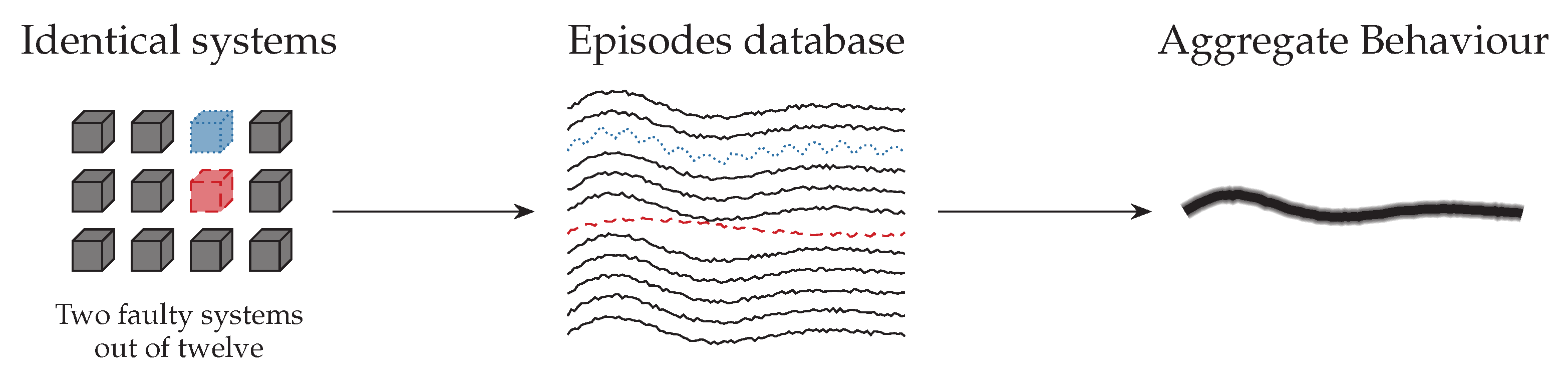
In this paper, we propose to solve this problem by training an “aggregate” model using historical data from a large number of identical or similar systems. Systems whose behaviour significantly deviates from the aggregate behaviour are detected as anomalous. While we cannot ensure that all systems work correctly, we assume that only a small part of them is faulty and that they are not affected by the same fault. Therefore, the individual faults would have a small impact during training, and the resulting model would be largely unaffected.

3. Consensus-Based Method for Anomaly Detection

The method proposed in this paper analyzes time-series from multiple similar systems. Correct and anomalous conditions are defined based on the consensus from all the systems.

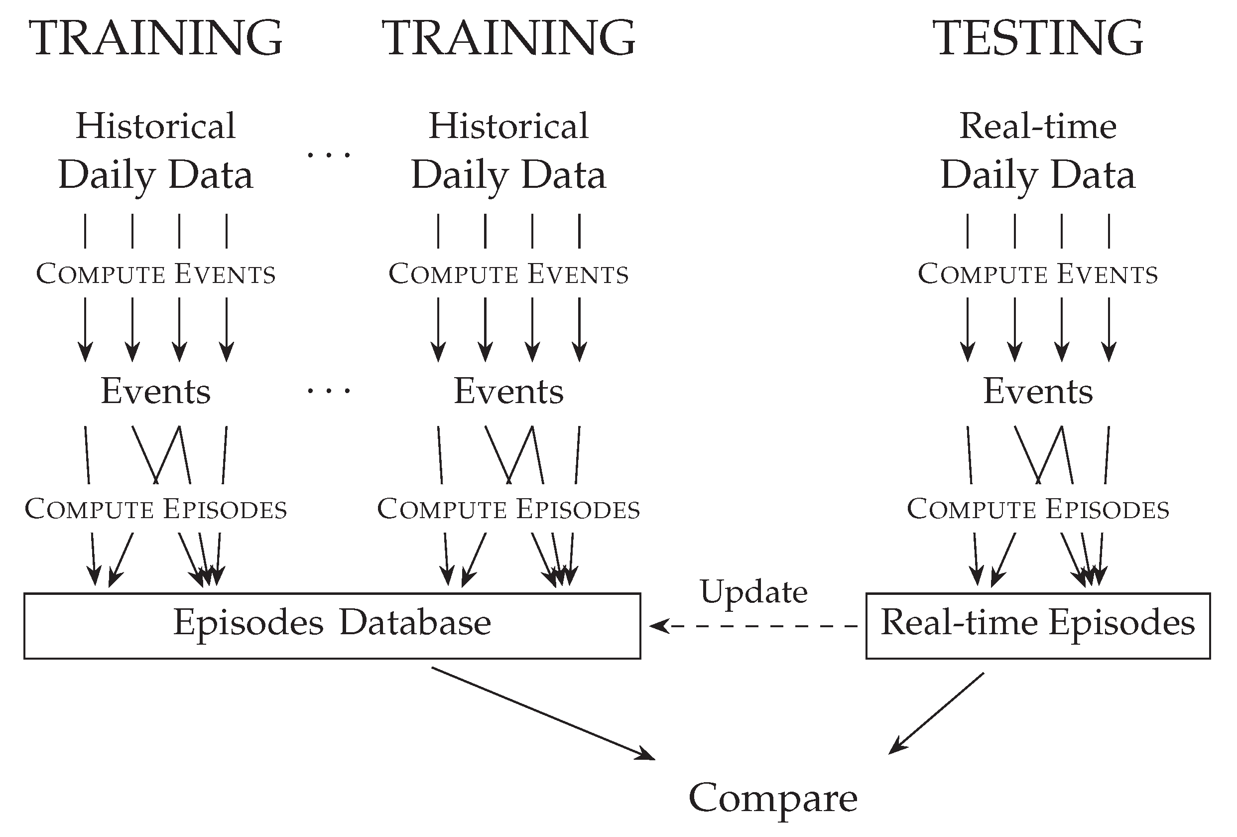
The main intuition of this method, illustrated in Figure 1, is to find sequences of events in multiple, related time-series and group them in episodes, where each episode represents a qualitative phenomenon. e.g., if CO₂ level rises, then the ventilation flow rate should increase, due to the BMS acting to maintain good air quality. Episodes are, therefore, a sequence of events belonging to a group of time-series. A database of episodes is obtained from historical data from several groups of time-series. Frequent episodes are assumed to happen during correct conditions, while rare or unknown episodes are assumed to be symptoms of anomalous behaviour. Episodes are later computed from real-time data and compared with the episodes in the database. When a large part of real-time episodes corresponds to episodes rarely encountered in historical data, i.e., when the current behaviour of the system is qualitatively different from its historical one, the system is flagged as anomalous.

The episode database can optionally be updated with new episodes computed from real-time data. This would allow to track seasonal variations and, moreover, to apply the method on a newly deployed system without using a separate training phase. In that case, the episodes database would be gradually populated over time, and earlier results could be inaccurate.

In order to avoid the necessity of validated fault-free training data, consensus between multiple similar systems can be exploited. Assuming that only a small part of the systems used in training are faulty or exhibit anomalous behaviours, their episodes would be overwhelmed by the episodes of the rest of the systems, as illustrated in Figure 2.

In order to obtain a consistent common behaviour, systems should be grouped by common characteristics. e.g., multiple rooms could be divided by room type, but also by room location, such as by floor number or building side, or by other characteristics. When a room shows anomalous behaviour within its group, it could be due to faulty components, but also to incorrect or insufficient grouping, as shown by Narayanaswamy et al. in Reference [9]. e.g., the only classroom on the top floor might deviate from all other classrooms, which are on the ground floor, due to different thermal loss. Multiple orthogonal characteristics should be used to avoid this possibility, such that systems which are anomalous in several groups are effectively labeled as anomalous.

Compared with a traditional approach of clustering based on model or statistical parameters, such as mean or variance, using episodes allows to represents interactions between different measurements over time. Such interactions, or lack thereof, can be qualitatively linked to physical phenomena within the system, and are learnt from aggregate historical data. Moreover, when updating the episodes database with episodes computed from real-time data, this method adapts to slow seasonal variations in the system’s dynamics.

In the rest of this section, we describe the procedure for data preprocessing and preparation, we define events and episodes, and, finally, we describe how to monitor multiple time-series to detect anomalies.

3.1. Data Preprocessing and Preparation

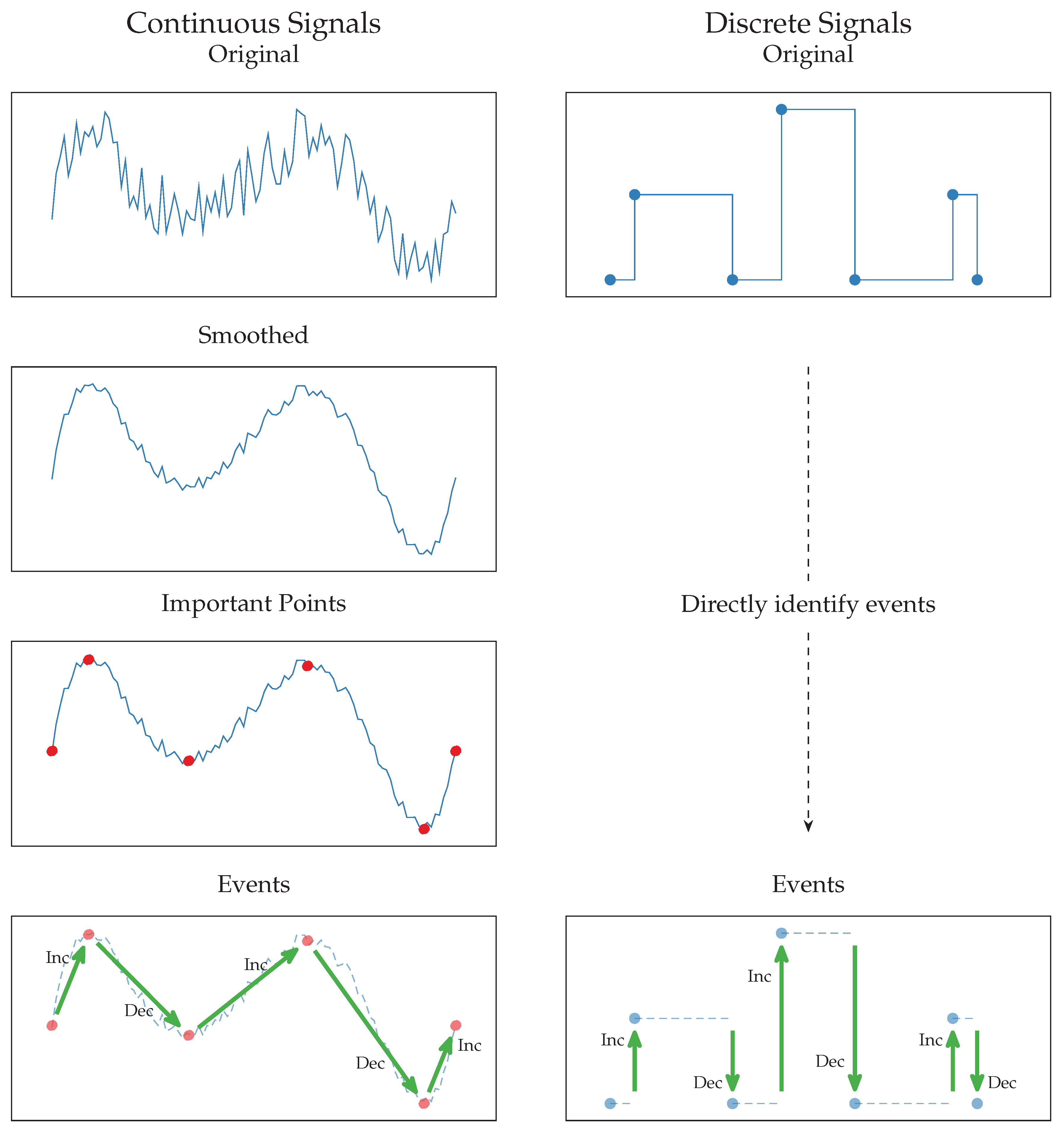
Time-series can be divided into two categories depending on the nature of the measured quantity. Time-series with a large number of readings changing gradually over time, such as temperature or CO₂ level, are called continuous time-series. Time-series with values defined over a finite and small domain, such as on/off, or a predetermined number of states, which are constant for long periods and change value abruptly, are instead called discrete time-series.

In order to extract episodes from a group of time-series, it is first necessary to extract events from each of them. An event is a qualitative local trend of a time-series. Events are defined and extracted differently for continuous and discrete time-series, as illustrated in Figure 3 and described in the following.

3.1.1. Events for Continuous Time-Series

The following method, based on the one presented by de Pisón et al. in [19], is used to extract events from continuous time-series.

Continuous time-series have many readings and are often subject to noise. In order to identify the high-level trend without accounting for small deviations, the time-series are first filtered with a lowpass filter. This operation is necessary to leave out low-order variations that do not impact significantly the system under test.

The next step is to find important points in time-series, which are defined as follows. Consider a time-series $a_i$, where $i\in \mathbb{Z}$ is the time index, and $a_i$ is the value at time index i, e.g., temperature in °C or CO₂ level in $\mathrm{ppm}$. Consider a point $a_m\in \mathrm{time}-\mathrm{series}$ and a window around it of radius n: $\left[a_{m-n},\dots ,a_m,\dots ,a_{m+n}\right]$. $a_m$ is an important minimum if and only if

$$\begin{array}{c}{a}_m=min\left[a_{m-n},\dots ,a_{m+n}\right],\hfill \\ \frac{a_i}{a_m}\ge r\wedge \frac{a_j}{a_m}\ge r\forall i,j:m-n\le i\le m\le j\le m+n,\hfill \end{array}$$

(1)

where $r⪈1$ is a compression factor. The closer is r to 1, the more important points are found. The precise value of r is a parameter that must be tuned for the specific experiment. Similarly, $a_m$ is an important maximum if and only if

$$\begin{array}{c}{a}_m=max\left[a_{m-n},\dots ,a_{m+n}\right],\hfill \\ \frac{a_m}{a_i}\ge r\wedge \frac{a_m}{a_j}\ge r\forall i,j:m-n\le i\le m\le j\le m+n.\hfill \end{array}$$

(2)

Once important points have been computed, it is possible to extract events. An event is a transition between two consecutive important points $a_k$ and $a_{\ell }$. In this paper, we consider the following event types: increment, decrement and horizontal trend. A transition is labeled as an increment if and only if

$$\begin{array}{c}{a}_k\mathrm{is}\mathrm{an}\mathrm{important}\mathrm{minimum}\hfill \\ a_{\ell }\mathrm{is}\mathrm{an}\mathrm{important}\mathrm{maximum}\hfill \\ w_1\le \ell -k\le w_2\hfill \\ h_1\le a_{\ell }-a_k\le h_2,\hfill \end{array}$$

(3)

where $w_1,w_2$ are constraints on the length of the transition and $h_1,h_2$ are constraints on the size of the transition. The constraints $w_1,w_2$ are measured in number of samples or, equivalently, in length of time intervals, when the time-series has a fixed sampling rate. The constraints $h_1,h_2$ are measured in the same unit of the time-series values, e.g., °C for time-series recording temperature, or $\mathrm{ppm}$ for time-series recording CO₂ level. Similarly, a transition is labeled as a decrement if and only if

$$\begin{array}{c}{a}_k\mathrm{is}\mathrm{an}\mathrm{important}\mathrm{maximum}\hfill \\ a_{\ell }\mathrm{is}\mathrm{an}\mathrm{important}\mathrm{minimum}\hfill \\ w_1\le \ell -k\le w_2\hfill \\ h_1\le a_k-a_{\ell }\le h_2.\hfill \end{array}$$

(4)

A transition is labeled as a horizontal step if and only if

$$\begin{array}{c}{a}_k,a_{\ell }\mathrm{are}\mathrm{important}\mathrm{points}\hfill \\ w_1\le \ell -k\le w_2\hfill \\ \left|a_k-a_{\ell }\right|\le h_2.\hfill \end{array}$$

(5)

3.1.2. Events for Discrete Time-Series

Extracting events from discrete time series is considerably simpler than from continuous ones. Discrete time-series measure logical quantities and are not affected by noise, therefore, no filtering is necessary. Moreover, filtering a discrete time-series would result in a continuous time-series transitioning smoothly from one state to the other, which would not significantly approximate the original signal. Therefore, the filtering step is not performed for discrete time-series.

Since changes of values in discrete time-series represent a logical change in the measured quantity, the values themselves are important points, and the changes themselves are events, as shown in Figure 3.

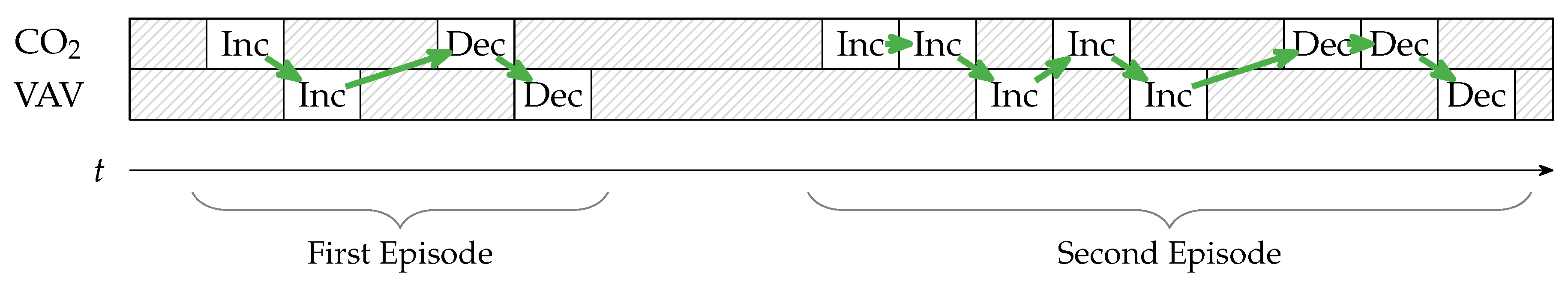
3.2. Episodes Involving Multiple Time-Series

Episodes are ordered chains of events pertaining to multiple time-series, as shown in Figure 4. They represent high-level cause-effect transitions, such as (Occupancy increases, CO₂ level increases, Ventilation increases), or (Ventilation increases, CO₂ level decreases). Episodes can contain any number of events but they are limited to a certain window size.

3.3. Monitoring Multiple Time-Series

The method consists of an initial training phase and an online detection phase (Figure 1). During the training phase, historical data are divided into daily chunks, and episodes are extracted from them and stored to a database. At the end of this phase, the majority of episodes in the database will represent usual behaviour of the system. In the online detection phase, episodes are extracted every day from data and compared to the ones in the database. All episodes that are absent in the database, or have less than a given probability, e.g., 5%, are flagged as anomalous. Therefore, when the system behaviour matches the one recorded in the database, it is considered normal, otherwise, it is considered anomalous.

A small number of anomalous episodes are expected even for healthy systems, therefore, a weekly moving average of anomalous episodes is computed. When such moving average exceeds a threshold, i.e., when anomalous episodes become common for a long period, the system as a whole is flagged as anomalous.

The method described so far can be used if validated and fault-free historical data is available. However, for many real-world systems, this might not be the case. If the system was faulty during the training period, the database would contain episodes representing faulty behaviour, and the method would flag such behaviour as correct during the online phase. This problem can be solved by exploiting consensus among several identical or similar systems during the training phase. Assuming most systems work correctly and only a small part are affected by faults, the majority of episodes stored in the database would, therefore, represent correct behaviour. Moreover, if faulty systems were affected by different faults their impact on the whole database would be even more diluted, as illustrated in Figure 2.

In order to account for slow-varying seasonal changes in the operation of the system, episodes obtained during the detection phase could be added to the database, and older episodes could be removed. In alternative, multiple databases could be created using historical data from different periods.

4. Case Study

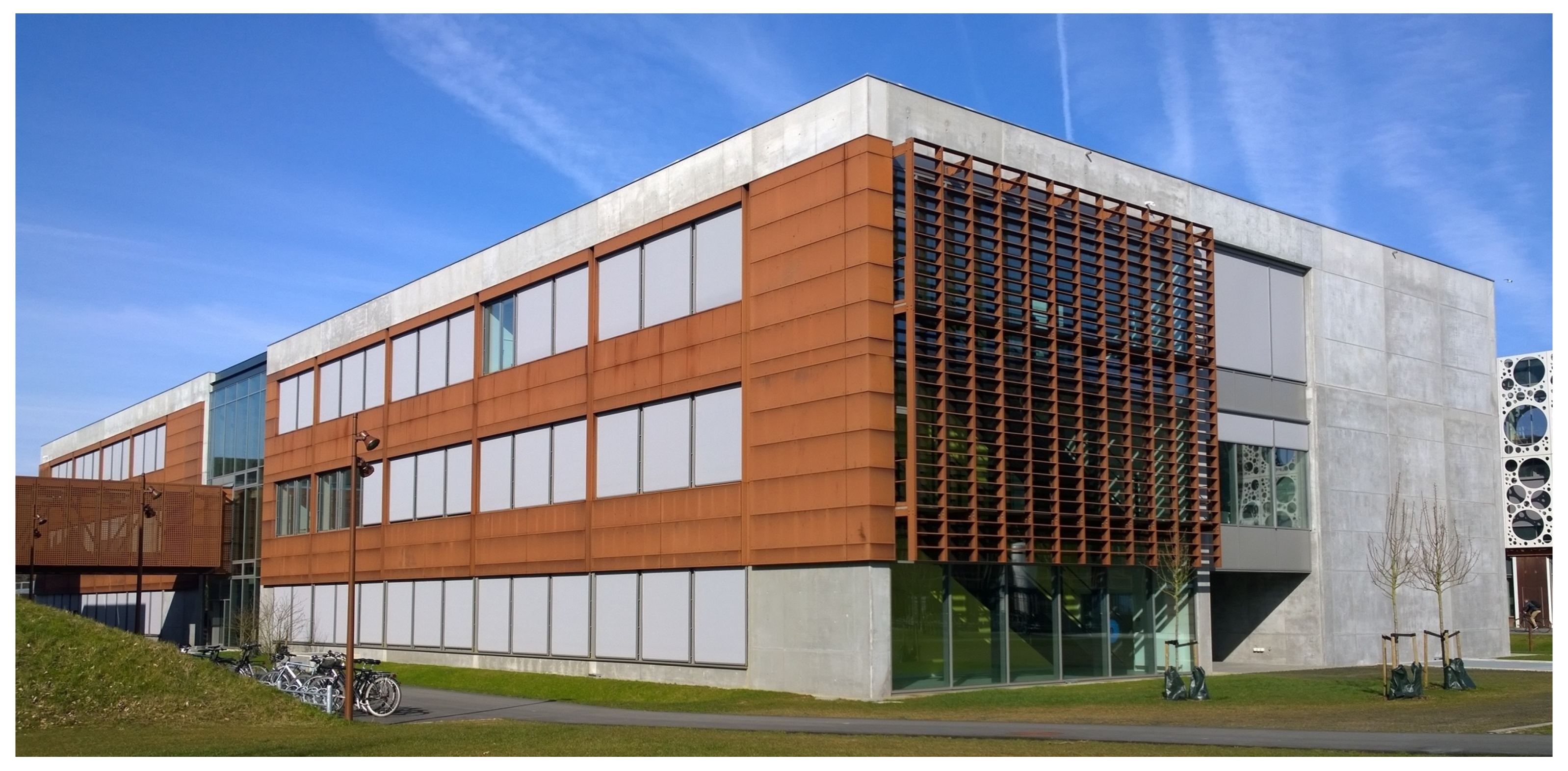
In this paper we present Odense Undervisning Building 44 (OU44) as a case study. The building, shown in Figure 5, is located at the main campus of University of Southern Denmark, in Odense. It was built in 2015 and it is mainly used for teaching and office work. The building contains around 120 rooms of different types, as shown in

Table 2. Room types in building OU44.

Room Type	Count	Room Type	Count
Office	48	Classroom	19
Corridor	21	Study zone	8
Other	7	Stairway	6
Conference room	4	Atrium	4
Copy room	3	Auditorium	2
Kitchen	2

, spread over three floors, and technical rooms located in the basement.

Data from the building are continuously recorded and stored in a database. Most rooms are equipped with indoor conditions sensors, such as CO₂ level, temperature, humidity and illuminance intensity, and with other meters such as lights status, heating valves and VAV units position, occupancy presence, blinds status and booking status. A selected number of rooms have separate plug load meters and occupancy counting cameras. In total, more than 3500 time-series are recorded for room-level measurements, and more than 1800 for the ventilation system.

The building’s ventilation system consists of four identical ventilation units, each of them serving one corner of the building (north-east, south-east, south-west and north-west). They are designed to maintain constant shafts pressures of 130 $\mathrm{Pa}$ and 40 $\mathrm{Pa}$ in the entire unit, while, at room level, supply flow rates depend on the VAV unit position. When VAV units are open, the pressure difference in the supply and extract shafts induce airflow in the room. The amount of open VAV units can be used as an estimate of the airflow required to maintain a constant pressure in the shafts, as was shown in Reference [20]. The airflow, in turns, is directly related to the energy consumption of the ventilation unit.

The position of VAV units themselves is based on multiple thresholds on CO₂ level: at 600 $\mathrm{ppm}$ the VAV unit opens by 45%, at 750 $\mathrm{ppm}$ it opens by 70% and at 900 $\mathrm{ppm}$ it opens by 100%. When CO₂ level decreases the thresholds are affected by hysteresis of 100 $\mathrm{ppm}$. The ventilation system is used to control room air quality, but also to provide natural cooling using outdoors air. As a result, VAV units can be open due to temperature, even when CO₂ level is low. Heating is provided by radiations, however, inlet air is heated to a setpoint of 20 °C–22 °C inside the ventilation units before entering the supply shaft.

Monitoring VAV Units

The BMS opens and closes VAV units to maintain room air quality, which is measured by the CO₂ level. When the VAV unit is working correctly, increasing its position results in higher ventilation, which reduces the CO₂ level in the room. It is difficult to accurately estimate the dependency between CO₂ level and VAV position. Previous attempts using regression models, such as the ones used in [9] for temperature control, lead to unsatisfactory results, perhaps due to the coarseness of VAV position with respect to CO₂ level. However, episodes involving the two time-series can capture the qualitative relation. Ventilation increasing due to cooling rarely occurs in Denmark, and only during summer months. Often, this happens when many occupants are in the room, which results in faster increase due to CO₂ level. Therefore, VAV position is dominated by CO₂ level, and the effect of temperature is small.

Rooms in the building were divided into four groups according to their corresponding ventilation unit. Events were extracted from two time-series, CO₂ level and VAV position ratio. Each group was used to train and generate a database of episodes. Under the assumption that rooms sharing the same ventilation unit have similar behaviour, the episodes are consistent within the group, and the resulting database contains similar episodes.

On the other hand, each ventilation unit serves different types of room, such as offices or classrooms. If a room type is underrepresented in the ventilation unit, the behaviour of such rooms might seem anomalous with respect to its peers. However, it would not be due to a fault, but instead to the room’s different shape and usage. To avoid this possibility of false positives, another experiment was performed by grouping rooms according to their type, as shown in Table 2.

Therefore, the groupings in the two experiments were defined as it follows.

(a)

Grouping by ventilation unit: the database was populated with episodes from all rooms belonging to the same ventilation unit. All four ventilation units 1 to 4 were considered.

(b)

Grouping by room type: the database was populated with episodes from all rooms of the same type. Six room types were considered: classroom, office, corridor, study zone, auditorium and conference room.

For both experiments, all parameters were set to the same values. Two time-series were considered: CO₂ level in the room and VAV position. The database was constructed dynamically, i.e., it was initially empty, and, every day, it was updated with episodes obtained during the online detection phase, and infrequent episodes were recorded. The experiment was performed on data from 20 November 2016 to 27 May 2017. Summer months were excluded, therefore, VAV position was independent of room temperature. Original data was resampled to 5 $\min$ and filtered with a Butterworth low-pass filter with cutoff period of 1 $\mathrm{h}$, as outlined in the step “Smoothed” in Figure 3. This type filter was chosen because its monotonously decreasing magnitude, which is flat in passband, does not distort the original signal [21,22]. The moving window size for episode search was set to 2 $\mathrm{h}$, and its step size was set to 10 $\min$ The minimal frequency ratio for anomalous episodes was set to 5%. Events were obtained using the following parameters. Transitions length constraints ($w_1$ and $w_2$ in Equations (3)–(5)) were set to 15 $\min$ and 120 $\min$. Transitions size constraints ($h_1$ and $h_2$ in Equations (3)–(5)) were set to 20 $\mathrm{ppm}$ and 30,000 ppm.

Table 3. Most frequent episodes in database for ventilation unit 1.

Rank	Episode	Count
1	Ventilation ↘, CO2 ↘	257
2	Ventilation ↗, CO2 ↘	252
3	Ventilation ↘, CO2 ↘, CO2 ↗	225
4	CO2 ↗, Ventilation ↘	223
5	CO2 ↗, Ventilation ↘, CO2 ↘	222
6	Ventilation ↗, CO2 ↗	219
7	CO2 ↘, Ventilation ↗, CO2 ↗	210
8	CO2 ↘, Ventilation ↗	203
9	Ventilation ↗, CO2 ↗, Ventilation ↘, CO2 ↘	169
10	Ventilation ↗, Ventilation ↘, CO2 ↘	160

shows the most frequent episodes in database for ventilation unit 1. Some episodes represent obvious qualitative behaviour of the ventilation system. e.g., ventilation is turned on for a while, then it is turned off, and CO₂ level decreases as a result (episode 10).

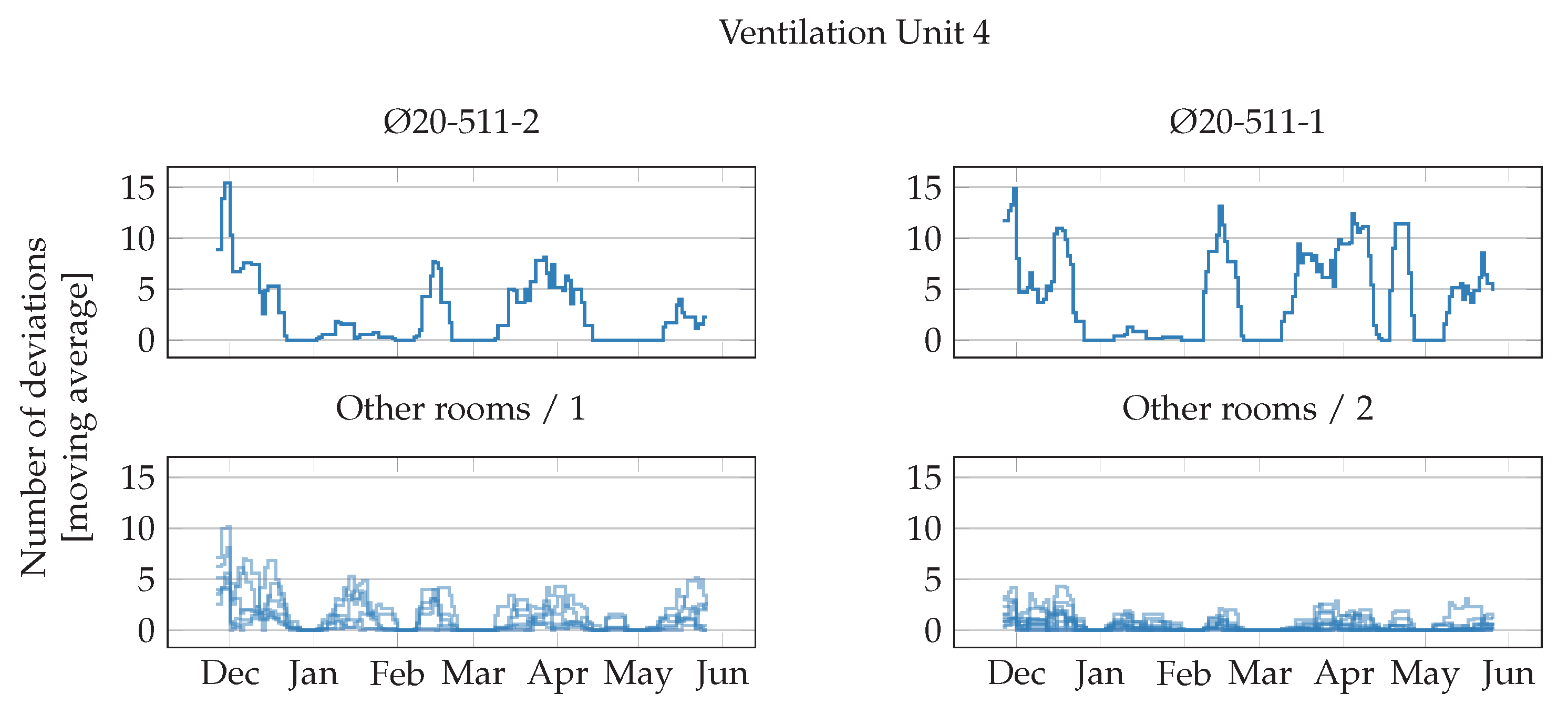
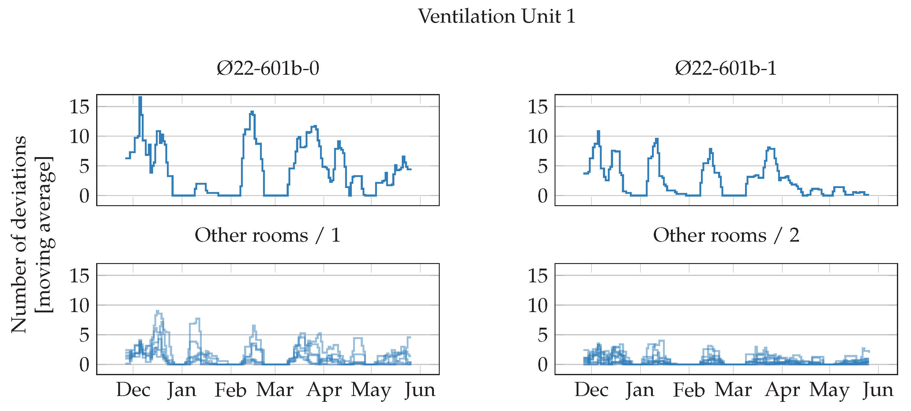
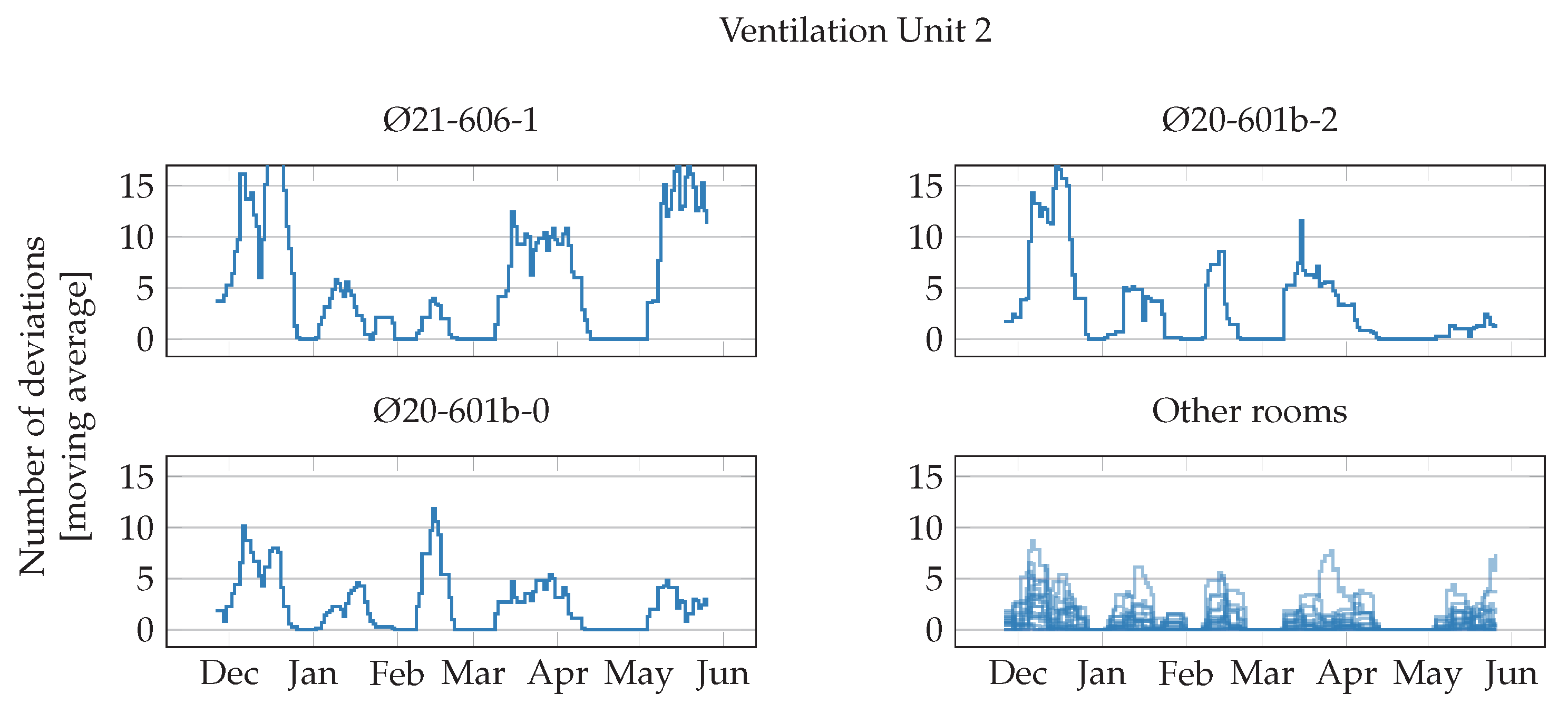
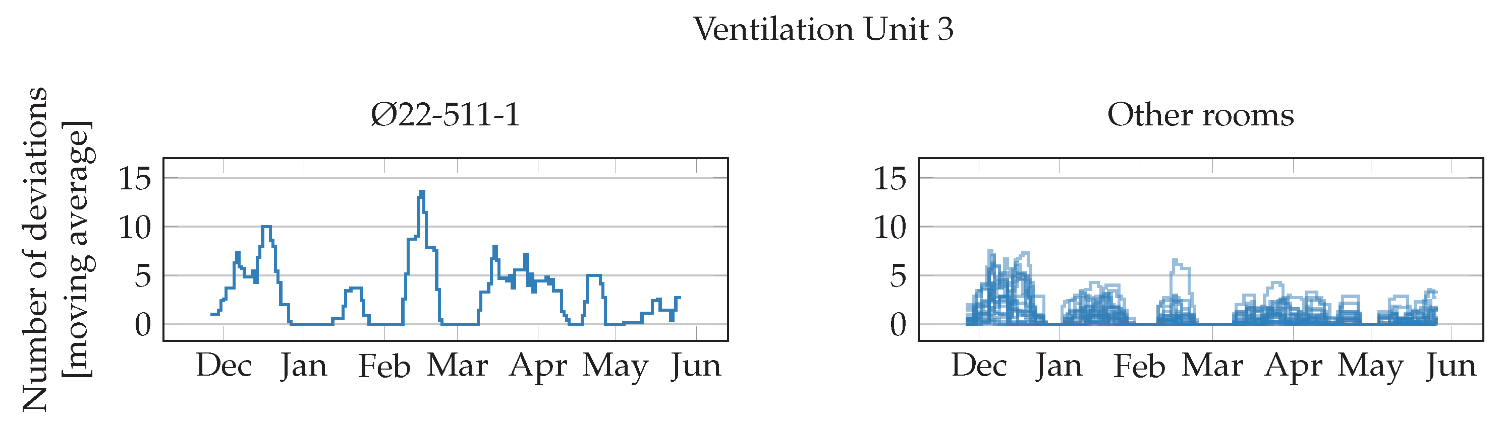
Figure 6, Figure 7, Figure 8 and Figure 9 show the weekly moving average of anomalous episodes for VAV units in rooms served by ventilation units 1 to 4. The rooms with the largest moving average are plotted separately in the first plots.

Table 4. Room flagged as anomalous in both experiments conducted.

Room type	Ventilation Unit
	Unit 1	Unit 2	Unit 3	Unit 4
Classroom	Ø22-601b-0	Ø20-601b-0, Ø20-601b-2		Ø20-511-1, Ø20-511-2
Auditorium	Ø22-601b-1		Ø22-511-1
Conference room		Ø21-606-1
Office
Study area
Corridor

summarizes the results of the two experiments: the same rooms were found anomalous whether they were grouped by ventilation unit, or by room type.

Figure 6 shows the results for the VAV units in rooms served by ventilation unit 1. The first two rooms, shown separately in the upper plots, have significantly more frequent anomalous episodes, i.e., episodes in these rooms differs more frequently from the episodes commons to all other rooms. Their moving average goes above 15 or it is often above 10, while for all other rooms it is consistently lower, i.e., they behave more similarly among each other.

Figure 7 shows the results for the VAV units in rooms served by ventilation unit 2. The moving average for the first two rooms is very large, it goes over 15 and it is often over 10. While never reaching 15, the moving average for the third room is also sometimes larger than 10, while all other rooms have lower values.

Figure 8 shows the results for the VAV units in rooms served by ventilation unit 3. In this case, only one room has moving average larger than 10, while all the others have lower values.

Figure 9 shows the results for the VAV units in rooms served by ventilation unit 4. The moving average for the first two rooms is very large, it goes over 15 and it is often over 10. All other rooms have lower values.

Figure 10 shows the results for the VAV units in classrooms. The five rooms which have the moving average over 10 are also the same that were found anomalous in the first experiment, when rooms were grouped by ventilation unit.

Table 4 summarizes the results of the two experiments. The same rooms were found anomalous whether they were grouped by ventilation unit or by room type, i.e., those rooms had a different behaviour compared to other rooms served by the same ventilation unit, and compared to other rooms of the same type. The anomalous rooms are 5 classrooms, two auditoriums and one conference room. Since the building contains only one auditorium and 4 conference rooms, the episode database, when grouping by room type, would contain episodes only for small amount of rooms. Therefore, the sample size is too small to conclude that the rooms have actually anomalous behaviour. Classrooms, however, are numerous in the building, and both experiments independently flagged the same rooms as anomalous.

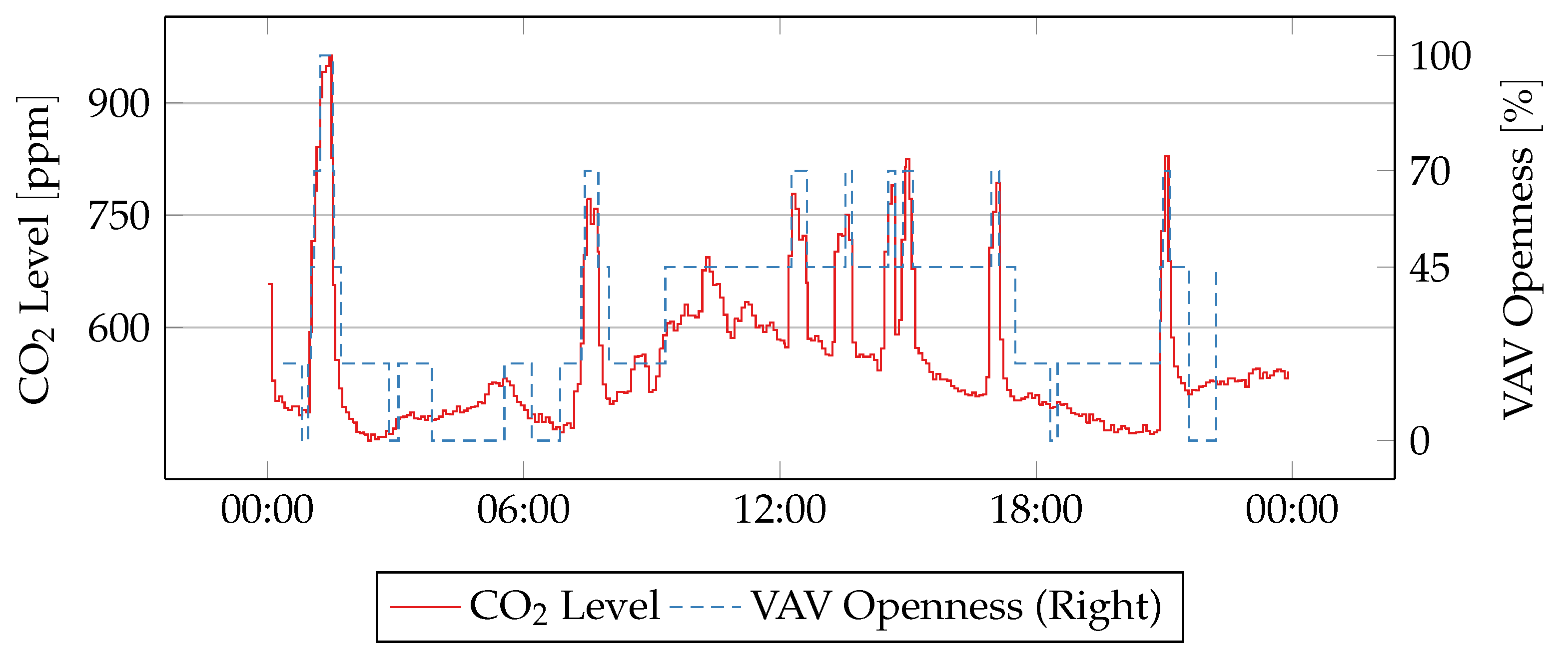
Figure 11 shows the values of CO₂ level and VAV position for room Ø21-606-1 on a day without anomalous episodes. Ventilation in the room follows CO₂ level as expected. The VAV unit opens by, respectively, 45 ppm, 70 ppm and 100 ppm when CO₂ level rises above 600 ppm, 750 ppm and 900 ppm. The VAV unit closes with some delay after the CO₂ level drops below the thresholds, due to hysteresis of 100 $\mathrm{ppm}$.

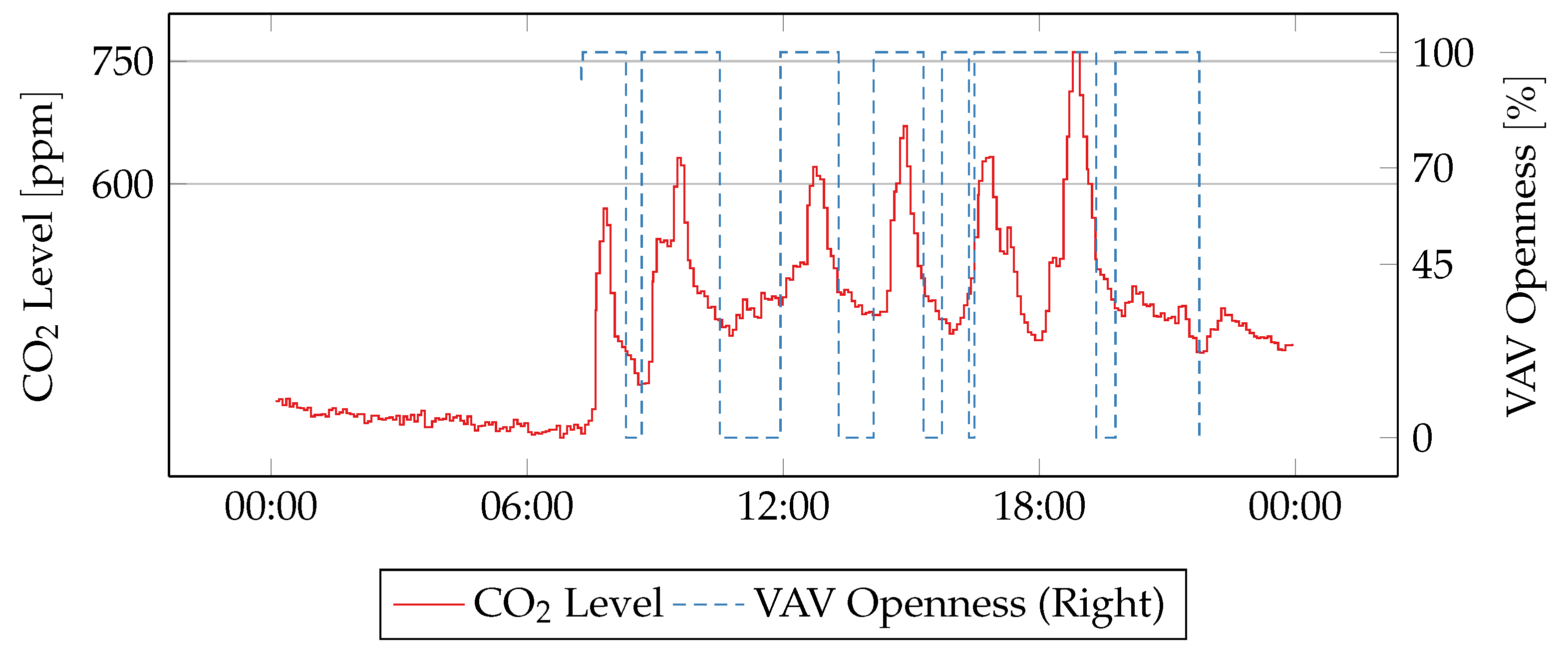
Figure 12 shows the values of CO₂ and VAV position for the same room on an anomalous day. CO₂ level is low during most of the day, and it only rises few times above the first thresholds of 600 $\mathrm{ppm}$. The VAV unit, however, always opens completely. High room temperature could cause ventilation to increase to provide natural cooling through outdoors air. However, room temperature never exceeds 24 °C during the day.

Finally, the moving average of deviations from common behaviour has an irregular trend. Some rooms, however, have a higher deviation at the beginning of the experiment, and, later, align themselves more to the other rooms. e.g., room Ø20-511-2, when clustering by ventilation unit and room type (Figure 9 and Figure 10), or room Ø20-601b-2, when clustering by ventilation unit and room type (Figure 7 and Figure 10). This might suggest that, during the first few weeks, the episodes database was not yet fully populated, and deviations during that period should be ignored.

5. Conclusions

In this paper, we presented a data-driven method for anomaly detection for VAV units based on consensus among several peers. A database of episodes is created from historical data and used to compute the frequency of new episodes. Compared to the majority of data-driven methods in the literature, the method does not need fault-free training data, instead, it relies on a large number of identical or similar systems. The effect of faulty systems during training is diluted over the entire dataset and, therefore, has a small impact on the generated model.

We applied the proposed method to detect anomalous VAV units of an existing building using CO₂ level and VAV position. Each room in the building contains a VAV unit, and all units are identical. We designed two experiments to investigate the behaviour of VAV units. At first, we grouped rooms by ventilation unit. Rooms served by the same ventilation unit are assumed to have the same behaviour, however, this assumption might not hold if their shape and usage are significantly different, and it is possible that they are incorrectly flagged as anomalous. Therefore, we ruled out this possibility by running a second experiment where we grouped the rooms by room type. The two experiments identified the same anomalous rooms, which suggests that their behaviour was, indeed, anomalous.

Some BMSs provide basic FDD capabilities, most often based on simple thresholds-based tests. Some faults at room level can be detected with these tests, e.g., a VAV unit stuck closed will eventually cause CO₂ level to rise above the threshold, however, they are not able to model complex dynamics. Episodes, on the other hand, can model interactions between different measurements, such as CO₂ level and VAV units positions, and, by using consensus, the proposed method can assess whether such interactions are similar to ones observed in their peers.

Consensus-based FDD methods are rarely applied in buildings systems. The proposed method is used to detect anomalies among interaction between VAV units and CO₂ level in the room. This approach shows the usefulness of using consensus between multiple similar systems to remove the need for fault-free historical data. Additional work would be necessary to decide whether anomalies are due to faults, misconfiguration or other causes, and, furthermore, to precisely diagnose such faults. The proposed method exposes several parameters, such as factor r, windows sizes, and thresholds for anomaly detection. In the experiments they were manually tuned to obtain a reasonable set of episodes, however, for a systematic application a method for self-tuning those parameters should be investigated.

The proposed method relies on the availability of many identical or similar components, and it can also be applied to other systems in buildings, such as heating, by monitoring episodes between radiators and room temperature, or lighting, by monitoring episodes between lights switches and illuminance sensors. More than two time-series can be used for phenomena that influence each other, such as CO₂ level, ventilation, temperature and heating, in order to generate more complex episodes.

Finally, the method presented in this paper was designed in the context of a complete framework for FDD and energy performance monitoring in buildings systems, aiming at developing a continuous monitoring application [23]. In our previous work, we addressed issues at different levels in buildings systems. Validation of sensors data through a basic set of rules and tests allows us to trust the status of the building, which is the basis for every advanced method using building’s data, and which is not always validated after construction [8]. By monitoring the whole building energy performance with a dynamic energy model, we can assess whether the building respects national regulations and attains its design goals, or if it suffers from unjustified increased energy consumption, and at which level [24]. When one of the building systems does not perform as expected, we can analyse its individual components to detect anomalous behaviour or deviations from past trends [20,25]. The method presented in this paper fills another area by isolating anomalous systems among multiple peers and, therefore, is another step towards a comprehensive FDD and energy performance monitoring framework for buildings.