Review

100 Years of Symmetrical Components

Dipartimento Energia “Galileo Ferraris”, Politecnico di Torino, corso Duca degli Abruzzi 24, 20129 Torino, Italy
*
Author to whom correspondence should be addressed.
Energies 2019, 12(3), 450; https://doi.org/10.3390/en12030450
Submission received: 31 December 2018 / Revised: 27 January 2019 / Accepted: 29 January 2019 / Published: 31 January 2019
(This article belongs to the Special Issue 10 Years Energies - Horizon 2028)

Abstract

:
28 June 2018 was the 100th anniversary of the first presentation on symmetrical components made by Charles LeGeyt Fortescue at the 34th Annual Convention of the American Institute of the Electrical Engineers in Atlantic City (NJ, USA). The introduction of the symmetrical component concept was immediately seen as a milestone for electrical system studies, and many applications have been developed during the ensuing years. Today, refined or advanced contributions to conceptual and practical aspects of electrical applications are still being proposed based on the powerful structure of symmetrical components. This paper recalls the most significant steps made in the electrical engineering field after the introduction of the symmetrical component theory, and indicates recent developments concerning the studies on electrical machines, harmonics and interharmonics in different applications, and the operation of power and distribution systems with distributed energy resources.

1. Introduction

The concept of symmetrical components introduced by Charles LeGeyt Fortescue represents one of the most useful transformations used in electrical circuit theory. A century ago, on 28 June 1918, the article “Method of Symmetrical Co-Ordinates Applied to the Solution of Polyphase Networks” was presented at the 34th Annual Convention of the American Institute of the Electrical Engineers in Atlantic City (NJ, USA). An insightful discussion followed the presentation, and six well-known experts argued about different aspects of Fortescue’s contribution. The article and the discussion were later published in the AIEE Transactions [1] and became a milestone for electrical engineers. Biographical notes about Fortescue are reported in various documents, including publications that celebrated anniversaries of the presentation in Atlantic City (25 years [2] and 80 years [3]) and further contributions [4].
The transformation in symmetrical components started with the studies that Fortescue initiated in 1913, referring to the operation of induction motors under unbalanced conditions for railway electrification applications [3]. The link between the symmetrical components and the electrical machines was then strongly established since the beginning [5]. On the other hand, in 1914 Stokvis also identified a synchronous system and an inverse system in his studies on synchronous machines operating in unbalanced three-phase systems [6], without considering the zero sequence [2]. In his discussion (by letter) of the Fortescue article presented in Atlantic City, Slepian indicated “the utility of the method is practically entirely limited to the case of rotating induction machines” [1]. In the same discussion, Slepian also suggested that the ratio between the negative sequence and the positive sequence is “a better quantity to denote the degree of unbalance of a line”; this unbalance factor was used by Fortescue in [7] and is still adopted today in the International Standards (e.g., [8]).
In the title of his article, Fortescue used the term “symmetrical co-ordinates”, and he used the terms “sequence components” and “symmetrical components” to indicate some of the entries resulting from the transformation. In the discussion, Karapetoff “incidentally” suggested the use of the expression “symmetrical components” instead of “symmetrical coordinates”. Even though Fortescue continued to refer to the overall framework using the term “symmetrical coordinates” [7], the expression “symmetrical components” became widely adopted worldwide, especially after the publication of the book Symmetrical Components by Wagner and Evans in 1933 [9]. The Wagner and Evans book also contains applications of symmetrical components to the study of short circuits and system disturbances.
The importance of symmetrical components grew so rapidly that the equipment data (for generators, lines, transformers, etc.) started to be provided in sequence components. Various discussions followed the wider use of the symmetrical components concept, for example concerning the symmetrical-component impedance notation [10] and the applications to transient analysis of symmetrical networks [11,12].
The main applications evolved with time, from the study of unbalanced conditions in rotating machines to the short circuit calculations in unbalanced systems (most of the system faults are unbalanced), up to the analysis of system transient stability and the operation of protection systems. In fact, the identification of the symmetrical components is very important for the operation of protection relays. The simplest case is that where all the ground relays operate by using zero-sequence quantities. A more elaborate example is the possibility of detecting the saturation of the current transformer by means of the formation of a third harmonic current component in the zero-sequence differential current [13].
The extraction of the symmetrical components was done first by using analog filters, that could be disturbed by direct current or harmonic components, as well as by the temperature and component aging. Then, with the advent of digital computer-based protection systems [14], the microprocessor-based solutions with digital filters increased their suitability to calculate the symmetrical components [15]. In the solution presented in [16], the sampling frequency must be a multiple of 150 Hz for a system with 50 Hz of fundamental frequency. These capabilities were further enhanced during the years. The solution presented in [17] implements the fast Walsh-Hadamard transform, and it is no longer necessary to have a sampling frequency multiple of 150 Hz. Further emerged solutions are mentioned in [18]. Furthermore, the Discrete-Wavelet transform was used in [19] to evaluate the symmetrical components with unbalanced and distorted waveforms in transient conditions. The advances also include the testing of new functionalities for the relays included in distribution systems [20]. The research in this direction is still open, with new emerging solutions such as the non-linear adaptive method proposed in [21] for the estimation of the symmetrical components in real-time.
The remaining sections of this article are structured as follows: Section 2 recalls the basic formulations of the Fortescue transformation for three-phase and polyphase systems, as well as the variants introduced to calculate the instantaneous symmetrical components and the generalised symmetrical components. Section 3 summarises the properties of the Fortescue transformation that are exploited for separating the sequences in electrical system studies. Section 4 addresses some recent applications to the analysis of harmonics and interharmonics. Section 5 deals with recent applications of the Fortescue transformation to the studies on electrical machines and distribution systems with distributed resources. The last section contains the conclusions.

2. Formulations of the Fortescue Transformation

The original formulation presented in [1] was written with many equations for n-phase systems. The formulation was then simplified by the introduction of the matrix form of the Fortescue transformation, which has been used in several computational methods [22].
In the discussion of Fortescue’s presentation at Atlantic City, Karapetoff suggested that the article would have been easier to follow by starting the presentation with the three-phase system and leaving the general case of n-phase systems for the following part of the article, a view supported by Mailloux, This suggestion is followed here to first synthesise some basic concepts.
For a three-phase system with phases a, b and c, let us consider the voltage phasors v a b c = [ V ¯ a , V ¯ b , V ¯ c ] T , where the superscript T denotes transposition. The Fortescue transformation is based on the definition of the sequences, indicated in the English literature as positive ( + ) , negative ( ) , and zero ( 0 ) with respect to the conventional counterclockwise sequence of phase rotation. In some cases, the numbers 1 and 2 have been used (e.g., as subscripts) to represent the positive and negative sequence, respectively. Curiously, a different terminology is traditionally used in the Latin languages (Table 1).
By using the complex operator α ¯ = e j 2 π 3 , the Fortescue transformation matrix is written as:
T = 1 3 [ 1 α ¯ α ¯ 2 1 α ¯ 2 α ¯ 1 1 1 ]
The transformed voltages v s = [ V ¯ ( + ) , V ¯ ( ) , V ¯ ( 0 ) ] T are then obtained as v s = T   v a b c , that is:
[ V ¯ ( + ) V ¯ ( ) V ¯ ( 0 ) ] = 1 3 [ 1 α ¯ α ¯ 2 1 α ¯ 2 α ¯ 1 1 1 ]   [ V ¯ a V ¯ b V ¯ c ]
The determinant of the transformation matrix is det ( T ) = α ¯ α ¯ 2 = j 3 . Since this determinant is non-null, the transformation matrix T is invertible, and the inverse matrix is:
T 1 = [ 1 1 1 α ¯ 2 α ¯ 1 α ¯ α ¯ 2 1 ]
with the property that T 1 = 3   T * T (the asterisk is the conjugation operator).
Furthermore, the unitary versions of the transformation matrices T ˜ and T ˜ 1 have been defined, with T ˜ 1 = T ˜ * T . Their application leads to the conservation of power from the space of the phase variables to the space of the sequence variables:
T ˜ = 1 3 [ 1 α ¯ α ¯ 2 1 α ¯ 2 α ¯ 1 1 1 ] ; T ˜ 1 = 1 3 [ 1 1 1 α ¯ 2 α ¯ 1 α ¯ α ¯ 2 1 ]
An interesting aspect is that the notion of sequence is a three-phase concept, and any quantity appearing in a sequence cannot exist only in one phase, but it must be in all three phases [23]. In other words, in the original and the transformed systems the number of variables must remain the same, even though one or more variables may be equal to zero under specific conditions.

2.1. Symmetrical Components for Polyphase Systems

The transformation matrix of order n (in the unitary version) is T n = 1 n A n , where A n n , n = { e j 2 π n i ( m 1 ) ,   i = 1 , , n ; m = 1 , , n } . The matrix A n is also a particular case of a Vandermonde matrix of order n, that is, V n = { v i m 1 ,   i = 1 , , n ; m = 1 , , n } , in which the generic term v i is replaced by e j 2 π n i [24]. The complex operator used can be represented as α ¯ n = e j 2 π n . For example, in the case n = 4 the complex operator is α ¯ 4 = e j π 2 , and the matrix A 4 becomes:
A 4 = [ 1 j 1 j 1 1 1 1 1 j 1 j 1 1 1 1 ]

2.2. Instantaneous Symmetrical Components

The extension of the symmetrical components to the time domain was presented in [25], leading to the so-called instantaneous symmetrical components (ISCs). In the ISCs, the complex operator α ¯ is still used, and the transformation matrix T is the same. The ISCs are complex quantities, used with their real and imaginary parts for the analysis. Starting from the phase voltages in the time domain v abc ( t ) = [ v a ( t ) , v b ( t ) , v c ( t ) ] T , the transformed voltages are defined as v s ( t ) = [ v ¯ ( + ) ( t ) , v ¯ ( ) ( t ) , v ( 0 ) ( t ) ] T = T   v abc ( t ) , where the components v ¯ ( + ) ( t ) and v ¯ ( ) ( t ) contain complex numbers, while the component v ( 0 ) ( t ) contains real numbers. Moreover, by definition the term v ¯ ( ) ( t ) = v ¯ ( + ) * ( t ) , so that the knowledge of the components v ¯ ( + ) ( t ) and v ( 0 ) ( t ) is sufficient to represent the ISCs [26]. The use of the complex operator α ¯ has also been replaced by a shift in the time domain corresponding to 2 π / 3 , in order to avoid the use of complex quantities to deal with time-domain waveforms [27].
The characteristics and advantages of using time-dependent symmetrical components in network calculations and the relations with other transformations for time-dependent signals are recalled in [28]. Useful aspects are the availability of the data in symmetrical components to model the network, and the simple relation between time-dependent symmetrical components and steady-state phasors that makes it easy to interpret the results. Some classical applications of ISCs include the modelling of dynamic phasors to analyse unbalanced faults in polyphase power systems [29], and to balance unbalanced loads and provide power factor correction [30]. The online estimation of steady state and ISCs in a three-phase system has been presented in [31], by using an extended phase-locked loop (EPLL). The EPLL provides the online estimation of the fundamental component of the input signal while following the variations of the signal in amplitude, phase and frequency, and is a key asset to enable the ISC assessment. The ISC transformation is used to generate the reference source currents corresponding to different strategies of load compensation [32]. Further recent developments concerning control of grid-side converters in microgrids are indicated in Section 5.

2.3. Generalized Symmetrical Components

The Generalized symmetrical components (GSC) have been introduced in [33]. The zero-sequence components are subtracted from the three-phase waveforms f a ( t ) ,   f b ( t ) and f c ( t ) (voltages or currents), obtaining the “heteropolar” components:
f ˜ a ( t ) = f a ( t ) f 0 ( t )
f ˜ b ( t ) = f b ( t ) f 0 ( t )
f ˜ c ( t ) = f c ( t ) f 0 ( t )
By indicating with T the period of the waveform, the generalized positive sequence component f ( + ) ( t ) is obtained by summing up the resulting waveforms of phase a, of phase b (shifted in time by −T/3) and phase c (shifted in time by −2T/3):
f ( + ) ( t ) = 1 3 ( f ˜ a ( t ) + f ˜ b ( t + T / 3 ) + f ˜ c ( t + 2 T / 3 ) )
The generalized negative sequence component f ( ) ( t ) is obtained by summing up the resulting waveforms of phase a, of phase b (shifted in time by T/3) and phase c (shifted in time by 2T/3):
f ( ) ( t ) = 1 3 ( f ˜ a ( t ) + f ˜ b ( t T / 3 ) + f ˜ c ( t 2 T / 3 ) )
The generalized zero sequence component f ( 0 ) ( t ) does not change with respect to the classical version:
f ( 0 ) ( t ) = 1 3 ( f a ( t ) + f b ( t ) + f c ( t ) )
From these definitions, the authors of [33] noted that, in non-sinusoidal cases, the three-phase waveforms could not be always obtained from the generalized positive sequence, negative sequence and zero sequence components. Thereby, a further component called the residual component was introduced for each phase:
f r a ( t ) = 1 3 ( f ˜ a ( t ) + f ˜ a ( t + T / 3 ) + f ˜ a ( t + 2 T / 3 ) )
f r b ( t ) = 1 3 ( f ˜ b ( t ) + f ˜ b ( t + T / 3 ) + f ˜ b ( t + 2 T / 3 ) )
f r c ( t ) = 1 3 ( f ˜ c ( t ) + f ˜ c ( t + T / 3 ) + f ˜ c ( t + 2 T / 3 ) )
The residual components have period T/3 and do not appear for sinusoidal waveforms. The mathematical relation among the GSCs and the symmetrical components introduced by Fortescue has been shown in [34].
Recent applications of the GSC have been provided in [35] to control three and four-leg inverters, and in [36] to construct the equivalent circuit for multiples of the third harmonic to determine the residual components in the three phases, from which the GSC application provides the exact results for the three phases in the analysis of unsymmetrical faults, also in particular cases with parallel connection of the sequence circuits.
The issues encountered in the definition of the generalised symmetrical components mainly refer to the treatment of the zero-sequence component. The same issue appears in the definition of the powers in unbalanced non-sinusoidal polyphase systems—largely debated in the scientific community. A recent solution proposed in [37] is to adapt the power definitions for polyphase systems in such a way that the zero-sequence components are not included.

3. Applications to Power and Distribution System Analysis

The fundamental property that has ensured the great success of the Fortescue transformation in electrical engineering studies is the diagonalisation of a matrix with circular symmetry. The structure of a generic matrix with circular symmetry is as follows:
A = [ a a a a a a a a a ]
If the matrix A describes a relation c = A b in the original space, the Fortescue transformation of the vectors b and c into b s = T   b and c s = T   c yields T 1   c s = A   T 1   b s , from which:
c s = T   A   T 1   b s = A s b s
where:
A s = [ a + α ¯ 2 a + α ¯ a 0 0 0 a + α ¯ a + α ¯ 2 a 0 0 0 a + a + a ]
In an electrical system, let us consider the impedance matrix Z abc that represents the relation v abc = Z abc i abc between the vector v abc that contains the phase voltage phasors and the vector i abc that contains the phase current phasors:
Z abc = [ Z ¯ 11 Z ¯ 12 Z ¯ 13 Z ¯ 21 Z ¯ 22 Z ¯ 23 Z ¯ 31 Z ¯ 32 Z ¯ 33 ]
The matrix Z abc is generally symmetrical, however the off-diagonal terms Z ¯ 12 , Z ¯ 13 and Z ¯ 23 could be different, and also the diagonal terms could not be all the same. In this case (e.g., for untransposed lines, typically found in distribution systems [38]) the impedance matrix Z s = T   Z abc   T 1 that results from the Fortescue transformation is not diagonal.
Due to the nature of the electrical circuit, the impedance matrix can be diagonalised only if all its diagonal terms are equal with each other (i.e., Z ¯ d = Z ¯ 11 = Z ¯ 22 = Z ¯ 33 ), and all the off-diagonal terms (mutual impedances) are equal with each other (i.e., Z ¯ m = Z ¯ 12 = Z ¯ 13 = Z ¯ 23 = Z ¯ 21 = Z ¯ 31 = Z ¯ 32 ). If this happens, the transformed matrix becomes:
Z s = [ Z ¯ d Z ¯ m 0 0 0 Z ¯ d Z ¯ m 0 0 0 Z ¯ d + 2 Z ¯ m ] = [ Z ¯ ( + ) 0 0 0 Z ¯ ( ) 0 0 0 Z ¯ ( 0 ) ]
and the three sequence circuits can be constructed separately for the symmetrical portion of the system. This property is at the basis of the study of the power system faults, where the sequence circuits are constructed separately, and the links among the circuits are established on the basis of the characteristics of the typical faults analysed [23]. The analysis of faults in a three-phase power system is then conducted by simply interconnecting the sequence networks in the appropriate way [39,40]. The topological method illustrated in [41] provides useful hints to understand the interactions among voltages and currents at different sequences.
In the construction of the sequence networks, the positive sequence network includes the whole system, that is, all the nodes are connected. The same happens for the negative sequence network. Conversely, in the zero sequence network the connection between nodes located at the terminals of a transformer depends on the type of windings and on the possible ground connection. It is possible to model the zero-sequence connections of the transformers in a simple way, by resorting to open and close switches [22]. As a result, the zero-sequence circuit can be composed of different non-interconnected areas. In the analysis of an unsymmetrical fault for different faulted points, the zero-sequence circuit to be considered may not be the same.
In some cases (e.g., in the presence of ground wires or bundle conductors) there are more than three conductors, however the impedance matrix may always be converted into a 3 × 3 matrix [22]. In these cases, as well as with untransposed lines (found in distribution systems), off-diagonal entries appear in the impedance matrix, and the sequence circuits cannot be decoupled. If the off-diagonal entries are much smaller than the diagonal entries, it is possible to use the average values of the diagonal entries and of the off-diagonal entries without introducing significant errors [22].
In the presence of untransposed lines, the coupling impedance between negative- and positive-sequence networks is considered, by separating the symmetric part of the impedance matrix from the coupling matrix that describes the mutual reactance variation between two phases due to the geometric asymmetry of the location of the conductors. In [38] this coupling impedance is used to determine the effects of different types of loads (constant current, constant impedance, constant power, and induction motor) on the voltage unbalances. In particular, it is shown that the presence of induction motor loads connected to Low Voltage (LV) increases the unbalance seen from the Medium Voltage (MV) busbars that supply the LV system, with respect to the other types of loads, because of the effects of the negative-sequence currents in the induction motor load. In [42] a circuit that represents the coupling due to line asymmetry is constructed by considering the positive and negative sequences.
In addition to the symmetry of the three-phase circuit, the decoupling of the sequences also requires that the power system components are linear and the waveforms are sinusoidal. The latter property makes it possible to analyse distorted waveforms separately in the harmonics domain, in which the waveforms are sinusoidal at each harmonic order (see Section 4).
If the matrix Z s is not diagonal, there is less practical advantage in transforming the electrical variables from the phase domain to the Fortescue domain. In [43] a fault calculation method based on the symmetrical components has been set up for active unbalanced distribution systems, showing that the fault calculations in the symmetrical component domain are faster than in phase coordinates (the execution time in symmetrical components is indicated to be between 34% and 56% of the one in phase coordinates). A method to calculate the solutions for complex short circuits that affect an arbitrary number of faulted nodes and phases is presented in [44].
The impedance of the zero-sequence circuit plays a key role in the analysis of unsymmetrical faults that involve the return path. In addition to the possible separation of the zero sequence networks, the type of transformer construction affects the numerical value of the zero-sequence impedance. In particular, the relevant distinction is among shell-type or core-type transformers. In shell-type transformers (or in the case of a three-phase transformer obtained by using three separate single-phase transformers), the magnetic circuits of each phase are reclosed in a path of relatively low reluctance, and the zero-sequence impedance of the transformer is the same as the positive sequence impedance. In core-type transformers with three legs, the magnetic flux provided by zero-sequence currents can only be reclosed through a path of relatively high reluctance (e.g., through the tank), and the zero-sequence impedance of the transformer is lower than the positive sequence impedance). With the traditional application of the symmetrical components it is then possible to explain in a simple conceptual and practical way why a single-phase fault at the secondary terminals of a core-type transformer with three legs can produce a fault current higher than the current that occurs for a three-phase fault at the same terminals.
Some limitations in the application of the symmetrical components occur in systems with multiple grounded points, in which the neutral is grounded in multiple points that are at different potential when a current flows in the return path. In this case, there are multiple paths for the return of the neutral current to the distribution transformer, leading to the presence of different currents whose value depends on the relative impedances on the grounding circuit. In this case, the symmetrical components can be applied only by assuming that the grounding conditions are uniform in the return path. The effects of individual grounding electrodes (that also depend on the ground resistivity, which may vary in different grounding points) cannot be represented. In [22] it is shown that significant errors may appear by using the symmetrical components with the uniform return path assumption in case of lines passing through areas with high resistivity.

4. Applications to Harmonic Analysis

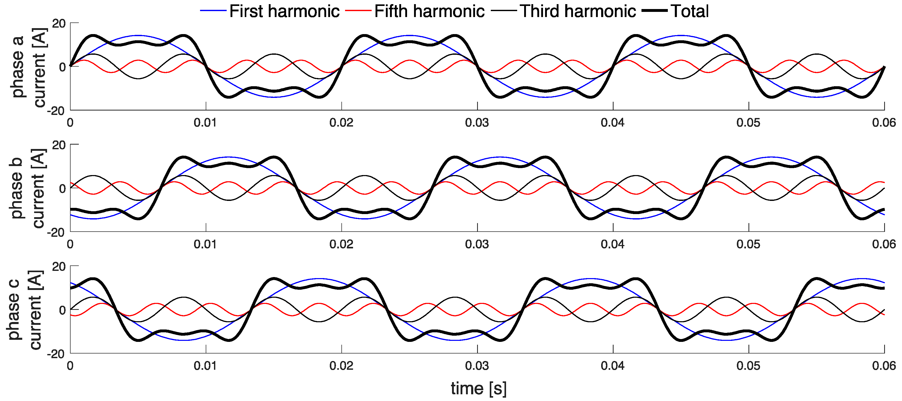
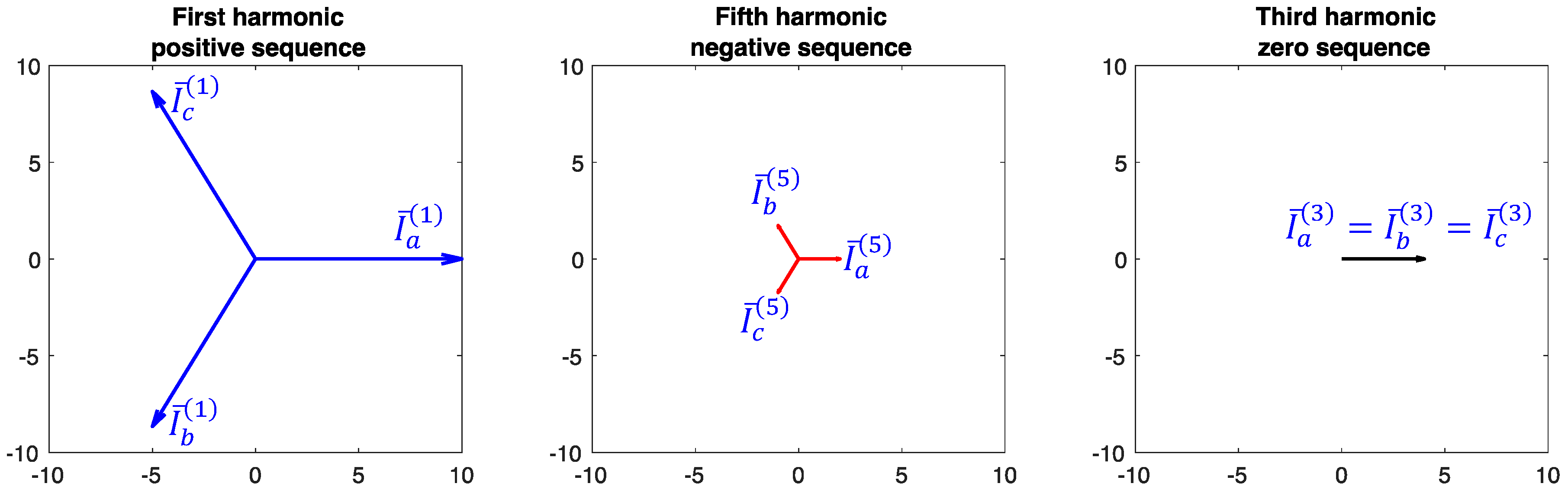
4.1. Symmetrical Components and Harmonics

A three-phase system is assumed to be balanced if the periodic waveform appearing on one phase (with period T, fundamental frequency f1 = 1/T, and fundamental radian frequency ω1 = 2πf1) is equal to the periodic waveforms appearing in the other two phases with a time shift of T/3 and 2T/3, respectively. This definition is generally valid also if the waveform is non-sinusoidal. The waveform distortion generates harmonics, and for the balanced three-phase system there is a simple relation between the harmonic order h = 0, 1, …, ∞ and the sequence that represents the phase voltages or currents (Table 2, in which the details of the sequences are also presented up to the harmonic order h = 40). This regularity is quite interesting and has been used to explain a number of phenomena appearing in the electrical systems. In particular, the harmonic orders 3h are called triplen harmonics and correspond to a zero sequence with the three phasors superposed with each other. In a balanced three-phase system with neutral, the triplen harmonics are the only components contributing to the neutral current. However, if the three-phase system is not balanced, the regularity indicated vanishes, and components of different sequences may appear at each harmonic order h > 0 [45]. These aspects have driven the researchers to look for the possibility of representing the balanced or unbalanced system conditions by using the measurements of the phasors gathered from a distorted periodic waveform at different harmonic orders. In particular, some links have been constructed between the transformation matrix used to calculate the symmetrical components and the determination of suitable components. For example, two components (denoted as first unbalance and second unbalance) have been introduced in [46] by applying different transformation matrices to the various harmonic orders. The system unbalance has then been obtained by combining these components. Conversely, in the Symmetrical Component Based (SCB) approach presented in [47] the balance, unbalance and distortion components are determined by using the same transformation matrix from phase quantities into symmetrical components. These components are calculated by summing the squares of the RMS values, because of the orthogonality of the components at different harmonic orders.
In the SCB approach, the current phasors i ( h ) = [ I ¯ a ( h ) , I ¯ b ( h ) , I ¯ c ( h ) ] T are transformed into i T ( h ) = T   i ( h ) = [ I ¯ T 1 ( h ) , I ¯ T 2 ( h ) , I ¯ T 3 ( h ) ] T . Then, the balance component of the phase current (subscript p) is calculated by collecting the contributions of the harmonic components that could exist in a balanced system for h = 1, …, ∞, that is, the harmonics of order 3h − 2 at the positive sequence (appearing from the transformed terms I ¯ T 1 ( 3 h 2 ) ), the harmonics of order 3h − 1 at the negative sequence (appearing in the transformed terms I ¯ T 2 ( 3 h 1 ) ), and the triplen harmonics (of order 3h − 3) at the zero sequence (appearing in the transformed terms I ¯ T 3 ( 3 h 3 ) ):
I p ( b ) = h = 1 [ ( I T 1 ( 3 h 2 ) ) 2 + ( I T 2 ( 3 h 1 ) ) 2 + ( I T 3 ( 3 h 3 ) ) 2 ]
The unbalance component of the phase current is calculated by considering all the complementary contributions obtained from the same transformation, that is, again with the RMS values:
I p ( u ) = h = 1 [ ( I T 2 ( 3 h 2 ) ) 2 + ( I T 3 ( 3 h 2 ) ) 2 + ( I T 1 ( 3 h 1 ) ) 2 + ( I T 3 ( 3 h 1 ) ) 2 + ( I T 1 ( 3 h 3 ) ) 2 + ( I T 2 ( 3 h 3 ) ) 2 ]
Finally, the distortion component of the phase current collects all the contributions at the harmonic orders higher than unity:
I p ( d ) = h = 2 [ ( I T 1 ( h ) ) 2 + ( I T 2 ( h ) ) 2 + ( I T 3 ( h ) ) 2 ]
The rationale used to choose the entries of the balance component is illustrated in the qualitative example shown in Figure 1, which represents three periods of a waveform with fundamental frequency f 1 = 50 Hz and period T = 0.02 s. For the sake of easy visualization, this example considers only the presence of three harmonics (of order 1, 3 and 5, with RMS values I ( 1 ) = 10 A, I ( 3 ) = 4 A, and I ( 5 ) = 2 A, respectively, and null initial angles for the harmonic currents at phase a). The three total currents are balanced, as the same distorted current waveform appears in the three phases at regular time shifts of T/3. Figure 2 shows the phasor diagrams. It is important to recall that the rotation of all phasors, including the ones of the negative and zero sequences, is counterclockwise. At the first harmonic, the phase currents [ I ¯ a ( 1 ) , I ¯ b ( 1 ) , I ¯ c ( 1 ) ] T = [ I ( 1 ) e j 0 , I ( 1 ) e j 2 π 3 , I ( 1 ) e j 2 π 3 ] T are transformed into [ I ¯ T 1 ( 1 ) , I ¯ T 2 ( 1 ) , I ¯ T 3 ( 1 ) ] T = [ I ( 1 ) , 0 , 0 ] T , that is, only the positive sequence entry is non-null. At the fifth harmonic, the phase currents [ I ¯ a ( 5 ) , I ¯ b ( 5 ) , I ¯ c ( 5 ) ] T = [ I ( 5 ) e j 0 , I ( 5 ) e j 2 π 3 , I ( 5 ) e j 2 π 3 ] T are transformed into [ I ¯ T 1 ( 5 ) , I ¯ T 2 ( 5 ) , I ¯ T 3 ( 5 ) ] T = [ 0 , I ( 5 ) , 0 ] T , that is, only the negative sequence entry is non-null. Finally, at the third harmonic, the phase currents [ I ¯ a ( 3 ) , I ¯ b ( 3 ) , I ¯ c ( 3 ) ] T = [ I ( 3 ) e j 0 , I ( 3 ) e j 0 , I ( 3 ) e j 0 ] T are transformed into [ I ¯ T 1 ( 3 ) , I ¯ T 2 ( 3 ) , I ¯ T 3 ( 3 ) ] T = [ 0 , 0 , I ( 3 ) ] T , where only the zero-sequence entry is non-null. The specific contribution of the individual harmonics can be seen from the evolution in time of the waveforms. The notion of balanced currents is well known for the first harmonic (and can be extrapolated to the harmonics corresponding to a positive sequence). The balanced nature of the third harmonics can be understood from their identical waveforms appearing in the three phases. Conversely, in general the interpretation of the balanced contribution of the harmonics corresponding to a negative sequence may be not intuitive. For this purpose, Figure 1 clarifies how the fifth harmonics in the three phases start from the phasor situation depicted in Figure 2 and evolve in time in such a way to provide the same contribution to the three phase currents, thus maintaining the overall balance.
Individual components can also be determined. For example, the balance component of the phase current at fundamental frequency is I p ( b 1 ) = I T 1 ( 1 ) , and the distortion component of the balance phase current is I p ( b d ) = ( I p ( b ) ) 2 ( I p ( b 1 ) ) 2 . Likewise, the unbalance component of the phase current at fundamental frequency is I p ( u 1 ) = ( I T 2 ( 1 ) ) 2 + ( I T 3 ( 1 ) ) 2 , and the distortion component of the unbalance phase current is I p ( u d ) = ( I p ( u ) ) 2 ( I p ( u 1 ) ) 2 .
Significant outcomes of the SCB approach are the definition of two indicators that provide a generalisation of the classical indicators used in many applications and Standards. The Total Phase current Distortion (TPDI) generalises the classical Total Harmonic Distortion (THD) indicator (calculated for each individual waveform) to provide a single indicator for the unbalanced three-phase system. The distortion component of the phase current is divided by the phase current components at fundamental frequency:
T P D I = I p ( d ) ( I p ( b 1 ) ) 2 + ( I p ( u 1 ) ) 2
Furthermore, the Total Phase current Unbalance (TPUI) generalises the classical unbalance indicator (defined as the ratio between the negative and the positive components at fundamental frequency) to take into account distorted currents:
T P U I = I p ( u ) I p ( b )
The SCB approach includes the determination of the components due to phase balance, unbalance and distortion for the voltages and for the neutral current [47].
The SCB framework has been used to identify suitable components and indicators associated to balance, unbalance and distortion referring to the triplen harmonics only [48]. In this way, it is possible to quantify to what extent the triplen harmonics contribute to the system balance or unbalance in particular situations occurring in unbalanced systems. For example, the triplen harmonics may be found in the phase currents also in a three-phase system without neutral. Moreover, triplen harmonics may appear in the phase currents even in a circuit located upward with respect to the delta-connected windings of a transformer.

4.2. Extension to Interharmonics

The IEC 61000-4-7 standard [49] indicates how to carry out measurements of harmonics and interharmonics. The waveform has to be sampled for 200 ms, corresponding to 10 periods at the fundamental frequency f 1 = 50 Hz. For the harmonic order h = 0, 1, …, H, let us consider the variable f h with frequency variation step Δ f h (e.g., Δ f h = 50   Hz , so that f h = h   f 1 ). Let us further consider another variable f ˇ z for z = 0, 1, …, N z , with frequency variation step Δ f ˇ z Δ f h and N z H . The variable z represents the interharmonic order when the corresponding frequency f ˇ z is different with respect to any harmonic frequency f h .
In [50] the findings of [46] have been used to determine the system unbalance with distorted waveforms by taking interharmonics into account, with different transformation matrices at each interharmonic order. This method has been applied in [51] to address how active power filters can compensate disturbances in the system. In [52] it has been established that if the consistency conditions N z = 10k H and Δ f h = 10 k   Δ f ˇ z are satisfied for any integer k = 1, 2, …, ∞, the application of the SCB approach (with a single transformation matrix) to the interharmonic orders z = 0, 1, …, N z assigns to the frequencies f h the same sequences provided by the application of the SCB approach to the harmonic orders h = 0, 1, 2, …, H (Table 3).
In this way, the SCB approach has been directly applied to the interharmonic case by transforming the phase current phasors i ( z ) = [ I ¯ a ( z ) , I ¯ b ( z ) , I ¯ c ( z ) ] T into i T ( z ) = T   i ( z ) = [ I ¯ T 1 ( z ) , I ¯ T 2 ( z ) , I ¯ T 3 ( z ) ] T and calculating the balance component I p ( b ) , unbalance component I p ( u ) , and distortion component I p ( d ) as:
I p ( b ) = z = 1 N Z [ ( I T 1 ( 3 z 2 ) ) 2 + ( I T 2 ( 3 z 1 ) ) 2 + ( I T 3 ( 3 z 3 ) ) 2 ]
I p ( u ) = z = 1 N Z [ ( I T 2 ( 3 z 2 ) ) 2 + ( I T 3 ( 3 z 2 ) ) 2 + ( I T 1 ( 3 z 1 ) ) 2 + ( I T 3 ( 3 z 1 ) ) 2 + ( I T 1 ( 3 z 3 ) ) 2 + ( I T 2 ( 3 z 3 ) ) 2 ]
I p ( d ) = z = 1 z 10 k N Z [ ( I T 1 ( z ) ) 2 + ( I T 2 ( z ) ) 2 + ( I T 3 ( z ) ) 2 ]
With these components, the interharmonics-based TPD and TPU indicators have been calculated as in the SCB approach. Specific applications are reported in [52] for k = 1 (with frequency variation step Δ f ˇ z = 5 Hz) and for k = 2 (with frequency variation step Δ f ˇ z = 0.5 Hz).

5. Recent Applications of the Fortescue Transformation

The applications of the Fortescue transformation are continuing in different areas of electrical engineering. In addition to the new proposals already indicated in the previous sections, the notes reported below refer to recent developments in progress in the studies of electrical machines and distribution systems with distributed energy resources (DERs).

5.1. Electrical Machines

In the study of the electrical machines, the use of the Fortescue transformation has recently addressed two different aspects. On the one hand, it has been used in the classical 3 × 3 form, applied in cases involving the stator of the classical three-phase machines. On the other hand, its generic n-form has been used for treating n-phase systems, with n > 3.
One of the most common applications found in the literature focuses on fault location and recognition in three-phase and n-phase drives. The principal faults can affect the electrical machine, the sensors or the power converter [53]. By focusing on the electrical machine faults, they can be further divided in stator faults and rotor faults. In this regard, many papers in the literature investigate these faults in the case of induction motors (IMs), due to their wide use in real world applications [54] for many years (Part II of Fortescue’s original paper already investigated the application to induction machines in an unbalanced polyphase system). For large IMs, the most relevant faults are related to the bearing (40%), followed by the stator winding breakdown (38%), broken rotor bar or end-rings (10%), and others (12%) [55,56]. Due to the presence of three-phase stator and multi-phase rotor, the Fortescue transformation is used for this kind of motors both in the classical and in the generalised form. In particular, [57] suggested a new expression of the stator currents of the IM in case of stator faults: the paper considered different stator faults (inter-turns short circuit, phase-to-phase, and single phase-to-ground faults). Through an analytical procedure, verified by experimental tests, it was demonstrated the effectiveness of choosing the phase angle and the magnitude of zero and negative sequence stator currents as indicators for the presence of stator faults under balanced voltage conditions. Other examples of use of the Fortescue transformation applied to the stator currents can be found in [58] and [59]. In particular, in [58] the symmetrical components of the stator current were used to implement a fault detection and diagnosis method, which in the first part extracts the features of the stator current that are used in the second step, where a classifier is adopted for discriminating the different types of faults, affecting both the stator and the rotor. The mechanical problems associated to the presence of oscillations on the load torque were analysed in [59]: also in this case, the stator currents, properly processed through the Fortescue transformation, were used for analysing the load torque of the motor, to identify oscillations that can highlight potential problems on the shaft of the IM. The symmetrical components of the stator currents were also used for detecting high-resistance connections (as in [60]), which can depend on the incorrect connection of different part of the drive.
The generic n-form transformation can be used for recognizing the presence of broken bars in the squirrel-cage of IM: for example, in [54] the authors used it for proving the existence of inverse order components, and thus implementing a detection method to localise the number of broken bars. In case of non-sinusoidal supply, the motor changes its behaviour and, due to this, dedicated methodologies have to be introduced. The presence of faults in case of non-sinusoidal supply can be highlighted through the methodology presented in [61]. The paper handled with bar-breakage fault detection and fault-gravity assessment, by presenting new classes of fault indicators, making use of the n-form version of the Fortescue transformation. The non-sinusoidal supply affects the efficiency of the IM, which can be investigated through the in situ estimation technique presented in [62]: in fact, in the presence of unbalanced supply conditions, the IM can be represented through positive and negative sequence circuits. A quite extensive modelling of the IM in symmetrical components for efficiency studies in unbalanced supply conditions was presented in [63]. The performance of the IM supplied from one-phase system was studied with the symmetrical components in [64]: the authors suggested a new schematic, providing the methodology for calculating the values of capacitances for guaranteeing higher efficiency than the ordinary single-phase IM.
New starting techniques were also investigated through the use of the classical 3 × 3 Fortescue transformation: for example, [65] presented a transient model of a three-phase IM started through the Field Aligned Starting (FAS) technique.
A further application regarding the IM and investigated through the use of the Fortescue transformation focuses on the self-excited induction generator (SEIG): in this application, the electrical machine acts as generator, and so it needs a self-excitation system able to create the rotor field. In [66] the general steady state analysis of the three-phase SEIG was presented, whereas a novel scheme for self-excitation was shown in [67].
For other types of motors, the main application is again fault detection. In [68], the use of the Fortescue transformation is the basis to derive analytical expressions for indicators referring to the inter-turn and phase-to-phase faults in permanent-magnet synchronous machines, allowing a concise representation of both the severity and the location of the fault. In the study of the winding faults for reluctance motors shown in [69], the Fortescue transformation is used in its generic form due to the presence of four phases. In [70], the three-phase transformation is used into an electrical signature analysis, consisting of the analysis of failure patterns in current or voltage spectra, which allows distinguishing the effects of mechanical and electrical faults on synchronous machine rotors.
Performance studies of non-conventional motors have been carried out by using the Fortescue transformation. The analysis of a linear resonant electrostatic induction motor is reported in [71]. The paper considers also the capacitive imbalance and indicates the correct way to design the electrodes in order to avoid the problems deriving from the capacitive effects. In the analysis of the line start permanent magnet synchronous motor illustrated in [72], thanks to the application of the 3 × 3 transformation, the authors analyse the steady-state behaviour of the machine, by comparing the theoretical results with experimental tests. Moreover, the Fortescue transformation is a valid analysis tool for linear motors: in particular, it can be used for investigating the electromagnetic thrust as shown in [73], in order to provide an overall evaluation of the longitudinal end-effects.
On the other hand, the Fortescue transformation has been used also for generalised n-phase symmetric electrical machines (characterised by voltage phasors shifted of 360°/n) [74]. Different contributions have addressed both the modelling and the control of multi-phase induction motors, as reported in [75]. More recently, a diagnostic fault classification for permanent magnet multi-phase motors has been presented in [76], in particular by investigating a 5-phase motor. The detection of the one-phase fault in 5-phase motor has been addressed in [77]: the authors considered the symmetrical components formulation both in normal operation and in fault operation, and, by comparing them, were able to detect the presence of the open-phase fault. An analysis of the effect of the stator winding connection for a 5-phase IM has been presented in [78]: also in this case, the n-form of the Fortescue transformation has been used.
Finally, the generic n-form formulation of the Fortescue transformation has been also used for designing the control of multi-phase inverters, having as goal the reduction of the phase current unbalance due to the use of symmetrical n-phase inverters [79].

5.2. Distribution Systems with Distributed Energy Resources

The increasing diffusion of DERs in the electrical networks has led to many advances in the modelling, analysis and control of the networks. DERs are inserted in distribution systems, which are typically unbalanced. As such, in the last years there has been an increasing interest in enhancing three-phase power flow and short circuit calculations, also incorporating more detailed model of DERs. A three-phase power-flow algorithm developed in the sequence component framework has been introduced in [80]. Appropriate sequence models have been constructed for DER sources, as well as for voltage-source converters (VSCs) connected to the grid [81]. The symmetrical component approach has been used in [82] in the presence of multiple converters inside a building, to generate the optimal references for the symmetrical component currents of all the converters. A more accurate representation of the sequence network circuit of the induction machine connected to wind generators, to be used in short circuit calculations, has been presented in [83]. The independent control of positive and negative voltage sequences in the compensation of unbalanced voltages by means of a static synchronous compensator (STATCOM) has been proposed in [84]. Different types of unbalance (structural, from partial shading, and mixed) have been characterised in [85] for photovoltaic (PV) systems operated with distorted waveforms by using the SCB approach. The control strategies used to inject the generated active power of a PV system into the grid, while providing also reactive power according with the grid code, have to be set up to operate in balanced and unbalanced conditions. A summary of control strategies that can be used to improve the performance of PV systems under unbalanced conditions has been presented in [86]. In the DC/AC control strategy, the choice of the reactive power reference for the control system depends on the positive and negative sequence components of the voltage at the point of common coupling (PCC). The current references are then determined on the basis of the power references and of the PCC voltage components at the positive and negative sequences.
In some applications, the reference currents are generated by considering symmetric voltages. Since in general the phase voltages are unbalanced and distorted, only the positive sequence component at fundamental frequency is extracted by using a three-phase Phase-Locked Loop (PLL) [87]. The PLL generates a periodic signal whose phase is related to the phase of a reference signal. A basic scheme of a PLL is shown in Figure 3. The three blocks are a phase detector (that compares the grid voltage phase angle θgrid with the PLL output θPLL, and determines the phase angle error θerror), a loop filter (i.e., a low-pass filter) that provides the radian frequency ωa, and the phase angle generator (a voltage controlled oscillator) that gives the phase angle θPLL. Various PLL types and their applications have been reviewed in [88] and [89]. One of the main issues for the PLL is the failure to operate properly in the presence of unbalanced grid faults, because of the presence of negative sequence components, and with possible harmonics. The techniques used to compensate the effects of unbalanced grid voltages are typically based on the addition of a pre-filtering stage in the voltage phase angle detector. An example is the Decoupled Double Synchronous Reference Frame PLL [90], where the grid voltage is first converted into separate positive and negative synchronous reference frames, then the voltages at the positive and negative sequences are extracted from the corresponding frame and are used to determine the grid voltage phase angle through a PLL. An enhanced version of the Decoupled Double Synchronous Reference Frame has been presented in [91], in order to control the positive sequence and negative sequence active and reactive powers independently of each other. Another solution to avoid the erroneous response of the PLL in the presence of negative-sequence components has been presented in [27], by making the sequence components available both as phasors in the frequency domain and as sinusoidal signals in the time domain. Analytical formulas have been proposed in [92] to analyse the effects of unbalance, harmonics, and interharmonics on the PLL. Further improvements of the PLL dynamics under unbalanced faults can be obtained by using Loop Filter Modification (LFM) methods, in which the loop filter block is modified or tuned depending on the fault or disturbance, in many different ways [89]. The negative-sequence components have been filtered from the unbalanced network voltages in [93], where an EPLL has been used to reduce the higher-order harmonics in converters connected to unbalanced networks. Furthermore, the PLL proposed in [94] is able to reject the negative sequence component, at fundamental frequency, the DC offset component, and the other harmonic components in the three-phase voltages.
A number of applications have been developed recently for the control of grid-side converters in microgrids. The converter that connects the local generation to the grid can be used in grid-sharing mode (to supply part of the local load) or in grid-injecting mode (by injecting power in the external network). Furthermore, multiple converters connected to the grid may operate independently or in a coordinated way.
The control of the converters requires the availability of the system variables in real time. For this purpose, in some applications the ISCs are used for generating the reference currents for the converters. In the control scheme proposed in [95], the reference currents are proportional to the power produced by the renewable energy sources and to the compensation requirement (e.g., null neutral current after compensation). In [96] the control algorithms developed on the basis of the ISCs operate a dual voltage source inverter in grid sharing and grid injecting modes. The control scheme presented in [97] includes a frequency-adaptive extractor of ISCs and harmonic components from the three-phase waveforms.
The accurate detection of the positive sequence component at fundamental frequency is essential to synchronise grid-connected three-phase converters [98]. A centralised control strategy for power sharing in a microgrid with grid-side converters operated in parallel has been proposed in [99], with reduced sensor requirements with respect to previous solutions. In an islanded microgrid that operates under unbalanced conditions, the asymmetric inverter output voltages could affect the droop control strategies. The droop control scheme has been adapted in [100] to obtain symmetrical three-phase reference voltage signals. The sharing of positive-, negative- and zero-sequence currents in islanded low voltage microgrids operating in unbalanced conditions has been addressed in [101] with the addition of virtual negative-sequence and zero-sequence impedance controllers.
In the DER operation, the current grid codes require that, in the presence of faults, the DER units must remain connected if the evolution of the voltage during the fault remains within given limits that define the fault ride-through (FRT) capability. For this purpose, the values of the positive and negative sequence components have to be available rapidly. However, many conventional methods (reviewed in [102]) are not sufficiently fast. A fast method to extract the symmetrical components for unbalanced three-phase systems has been proposed in [102] by using the non-nominal dq-transformation at frequency higher than the fundamental. A FRT control strategy based on positive/negative sequence droop control has been proposed in [103] to coordinate the power injection among multiple converters during voltage sags. Moreover, the variation of the voltage at the neutral point during FRT is a significant aspect for PV inverters, addressed in [104] with the definition of four weighting factors based on symmetrical components, which provide insights on the neutral point voltage fluctuation.

6. Conclusions

After 100 years, the symmetrical components introduced by Fortescue continue to be a fundamental tool for electrical engineers. The significant number of recent papers that propose further contributions indicates the advances in progress in the emergent sectors of development of the electrical engineering technologies and related applications. The various applications mainly refer to the studies on electrical machines and drives, and to the analysis of power and distribution systems.
In the case of electrical machines and drives, the Fortescue transformation is used for addressing various problems happening in different machines. In particular, the most common applications are (still) the operation under unbalanced conditions and the fault detection (both for stator and rotor faults). The symmetrical components are used for machine design and control, especially for new machines and innovative applications such as n-phase drives. The presence of non-sinusoidal waveforms due to the wider use of power electronics requires an extensive modelling of the electric machines in sequence components for studying the machine efficiency.
The power system applications refer to the modernisation under way towards smarter grids, also addressing power quality issues. Fortescue’s transformation is fundamental for properly implementing the protection schemes. Recently, due to the increase of the DER share in distribution systems, the Fortescue transformation has been used for addressing problems involving different aspects, from the modelling of the converters for grid connection of DERs to be used in power flow and short circuit calculations, to the enhancement of the solutions for providing better control of the converters, for either single converters or multiple coordinated converters connected to the distribution system or to a microgrid. The main issue remains the provision of real-time information on the DER operation in unbalanced systems, in normal or faulted conditions. A number of solutions have emerged to address the critical issue of the erroneous behaviour of the PLL under transient and unbalanced conditions. Furthermore, in the power quality domain the symmetrical components have been used to provide conceptual advances on the properties of different harmonics and interharmonics in unbalanced systems with distorted waveforms.
By summarising, the main strength of Fortescue’s transformation lies in the concept it introduced. Any new formulation developed for different applications of the symmetrical components still aims to reproduce the same “beautiful simplicity” highlighted by Slepian in his letter sent one century ago to comment on the original contribution presented by “Mr. Fortescue”.

Author Contributions

The authors have contributed equally.

Funding

This research received no external funding.

Conflicts of Interest

The authors declare no conflict of interest.

References

  1. Fortescue, C.L. Method of symmetrical co-ordinates applied to the solution of poly-phase networks (with discussion). Presented at the 34th Annual Convention of the AIEE (American Institute of Electrical Engineers), Atlantic City, NJ, USA, 28 June 1918; Volume 37, pp. 1027–1140. [Google Scholar]
  2. Wagner, C.F.; Butler, J.W.; Crary, S.B.; Hobson, J.E.; Huntington, E.K.; Johnson, A.A.; Kroneberg, A.A.; Miller, M.C.; Sels, H.K.; Trueblood, H.M. Silver anniversary of symmetrical components. Electr. Eng. 1943, 62, 294–295. [Google Scholar]
  3. Brittain, J.E.; Charles, L.G. Fortescue and the method of symmetrical components [Scanning the Past]. Proc. IEEE 1998, 86, 1020–1021. [Google Scholar] [CrossRef]
  4. Furfari, F.A. Charles LeGeyt Fortescue and the method of symmetrical components. IEEE Ind. Appl. Mag. 2002, 8, 7–9. [Google Scholar] [CrossRef]
  5. Kilgore, L.A. Calculation of Synchronous Machine Constants- Reactances and Time Constants Affecting Transient Characteristics. Trans. Am. Inst. Electr. Eng. 1931, 50, 1201–1213. [Google Scholar] [CrossRef]
  6. Stokvis, M.L.G. Sur la création des harmoniques 3 dans les alternateurs par suite du déséquilibrage des phases. In Proceedings of the Comptes Rendus Hebdomadaires des Séances de l’Académie des Sciences, Paris, France, 15 June 1914; Volume 159, p. 46. [Google Scholar]
  7. Fortescue, C.L. Polyphase Power Representation by Means of Symmetrical Coordinates. Trans. Am. Inst. Electr. Eng. 1920, 39, 1481–1484. [Google Scholar] [CrossRef]
  8. International Electrotechnical Commission. Electromagnetic Compatibility (EMC)—Environment—Compatibility Levels for Low-Frequency Conducted Disturbances and Signalling in Public Low-Voltage Power Supply Systems; Standard IEC 61000-2-2; IEC: Geneva, Switzerland, 2002. [Google Scholar]
  9. Wagner, C.F.; Evans, R.D. Symmetrical Components; Mc-Graw-Hill: New York, NY, USA, 1933. [Google Scholar]
  10. Kimbark, E.W. Symmetrical-component impedance notation. Electr. Eng. 1938, 57, 431. [Google Scholar] [CrossRef]
  11. Pipes, L.A. Transient analysis of symmetrical networks by the method of symmetrical components. Electr. Eng. 1940, 59, 457–459. [Google Scholar] [CrossRef]
  12. Pipes, L.A. Discussion of “Transient analysis of symmetrical networks by the method of symmetrical components”. Electr. Eng. 1940, 59, 1107–1110. [Google Scholar] [CrossRef]
  13. Villamagna, N.; Crossley, P.A. A CT saturation detection algorithm using symmetrical components for current differential protection. IEEE Trans. Power Deliv. 2006, 21, 38–45. [Google Scholar] [CrossRef]
  14. Phadke, A.G.; Ibrahim, M.; Hlibka, T. Fundamental basis for distance relaying with symmetrical components. IEEE Trans. Power Appar. Syst. 1977, 96, 635–646. [Google Scholar] [CrossRef]
  15. Phadke, A.G.; Thorp, J.S.; Adamiak, M.G. A New Measurement Technique for Tracking Voltage Phasors, Local System Frequency, and Rate of Change of Frequency. IEEE Trans. Power Appar. Syst. 1983, 102, 1025–1038. [Google Scholar] [CrossRef]
  16. Degens, A.J. Microprocessor-implemented digital filters for the calculation of symmetrical components. IEE Proc. C Gener. Transm. Distrib. 1982, 129, 111–118. [Google Scholar] [CrossRef]
  17. Sharma, P.; Ahson, S.I.; Henry, J. Microprocessor implementation of fast Walsh-Hadamard transform for calculation of symmetrical components. Proc. IEEE 1988, 76, 1385–1388. [Google Scholar] [CrossRef]
  18. Yazdani, D.; Mojiri, M.; Bakhshai, A.; Joós, G. A Fast and Accurate Synchronization Technique for Extraction of Symmetrical Components. IEEE Trans. Power Electron. 2009, 24, 674–684. [Google Scholar] [CrossRef]
  19. Morsi, W.G.; El-Hawary, M.E. On the application of wavelet transform for symmetrical components computations in the presence of stationary and non-stationary power quality disturbances. Electr. Power Syst. Res. 2011, 81, 1373–1380. [Google Scholar] [CrossRef]
  20. Petit, M.; Le Pivert, X.; Garcia-Santander, L. Directional relays without voltage sensors for distribution networks with distributed generation: Use of symmetrical components. Electr. Power Syst. Res. 2010, 80, 1222–1228. [Google Scholar] [CrossRef]
  21. Naidoo, R.; Pillay, P.; Visser, J.; Bansal, R.C.; Mbungu, N.T. An adaptive method of symmetrical component estimation. Electr. Power Syst. Res. 2018, 158, 45–55. [Google Scholar] [CrossRef]
  22. Das, J.C. Understanding Symmetrical Components for Power System Modeling, 1st ed.; Wiley Online Library: Hoboken, NJ, USA, 2017. [Google Scholar]
  23. Lewis Blackburn, J. Symmetrical Components for Power Systems Engineering; Marcel Dekker: New York, NY, USA, 1993. [Google Scholar]
  24. Yeung, K.S. A New Look at the Method of Symmetrical Components. IEEE Trans. Educ. 1983, 26, 68–70. [Google Scholar]
  25. Lyon, W.V. Transient Analysis of Alternating-Current Machinery; John Wiley: New York, NY, USA, 1954. [Google Scholar]
  26. Leva, S. Power Network Asymmetrical Faults Analysis Using Instantaneous Symmetrical Components. J. Electromagn. Anal. Appl. 2009, 1, 205–213. [Google Scholar] [CrossRef]
  27. Karimi-Ghartemani, M.; Karimi, H. Processing of Symmetrical Components in Time-Domain. IEEE Trans. Power Syst. 2007, 22, 572–579. [Google Scholar] [CrossRef]
  28. Paap, G.C. Symmetrical components in the time domain and their application to power network calculations. IEEE Trans. Power Syst. 2000, 15, 522–528. [Google Scholar] [CrossRef] [Green Version]
  29. Stankovic, A.M.; Aydin, T. Analysis of asymmetrical faults in power systems using dynamic phasors. IEEE Trans. Power Syst. 2000, 15, 1062–1068. [Google Scholar] [CrossRef]
  30. Ghosh, A.; Joshi, A. A new approach to load balancing and power factor correction in power distribution system. IEEE Trans. Power Deliv. 2000, 15, 417–422. [Google Scholar] [CrossRef]
  31. Iravani, M.R.; Karimi-Ghartemani, M. Online estimation of steady state and instantaneous symmetrical components. IEE Proc. Gener. Transm. Distrib. 2003, 150, 616–622. [Google Scholar] [CrossRef]
  32. Rao, U.K.; Mishra, M.K.; Ghosh, A. Control Strategies for Load Compensation Using Instantaneous Symmetrical Component Theory Under Different Supply Voltages. IEEE Trans. Power Deliv. 2008, 23, 2310–2317. [Google Scholar] [CrossRef]
  33. Tenti, P.; Willems, J.L.; Mattavelli, P.; Tedeschi, E. Generalized symmetrical components for periodic non-sinusoidal three-phase signals. Electr. Power Qual. Util. J. 2007, XIII, 9–15. [Google Scholar]
  34. Húngaro Costa, L.L.; Amaral Serni, P.J.; Pinhabel Marafão, F. An analysis of Generalized Symmetrical Components in non sinusoidal three phase systems. In Proceedings of the XI Brazilian Power Electronics Conference, Natal, Brazil, 11–15 September 2011; pp. 502–507. [Google Scholar]
  35. Liberado, E.V.; Pomilio, J.A.; Alonso, A.M.S.; Tedeschi, E.; Marafão, F.P.; Guerreiro, J.F. Three/Four-leg Inverter Current Control Based on Generalized Symmetrical Components. In Proceedings of the IEEE 19th Workshop on Control and Modeling for Power Electronics (COMPEL), Padova, Italy, 25–28 June 2018. [Google Scholar]
  36. Karami, E.; Gharehpetian, G.B.; Madrigal, M.; de Jesus Chavez, J. Dynamic Phasor-Based Analysis of Unbalanced Three-Phase Systems in Presence of Harmonic Distortion. IEEE Trans. Power Syst. 2018, 33, 6642–6654. [Google Scholar] [CrossRef]
  37. Mikulović, J.; Škrbić, B.; Đurišić, Ž. Power definitions for polyphase systems based on Fortescue’s symmetrical components. Int. J. Electr. Power Energy Syst. 2018, 98, 455–462. [Google Scholar] [CrossRef]
  38. Paranavithana, P.; Perera, S.; Koch, R.; Emin, Z. Global voltage unbalance in MV networks due to line asymmetries. IEEE Trans. Power Deliv. 2009, 24, 2353–2360. [Google Scholar] [CrossRef]
  39. Lyon, W.V. Applications of the Method of Symmetrical Components; McGraw Hill: New York, NY, USA, 1937. [Google Scholar]
  40. Clarke, E. Circuit analysis of A.C. Power Systems: Symmetrical Components; Wiley: New York, NY, USA, 1943. [Google Scholar]
  41. Gandelli, A.; Leva, S.; Morando, A.P. Topological considerations on the symmetrical components transformation. IEEE Trans. Circuits Syst. I Fundam. Theory Appl. 2000, 47, 1202–1211. [Google Scholar] [CrossRef]
  42. Bellan, D.; Superti-Furga, G.; Pignari, S.A. Circuit representation of load and line asymmetries in three-phase power systems. Int. J. Circuits Syst. Signal Process. 2015, 9, 75–80. [Google Scholar]
  43. Jabr, R.A.; Dzafic, I. A Fortescue approach for real-time short circuit computation in multiphase distribution networks. IEEE Trans. Power Syst. 2015, 30, 3276–3285. [Google Scholar] [CrossRef]
  44. Strezoski, L.; Prica, M.; Loparo, K.A. Sequence Domain Calculation of Active Unbalanced Distribution Systems Affected by Complex Short Circuits. IEEE Trans. Power Syst. 2018, 33, 1891–1902. [Google Scholar] [CrossRef]
  45. Desmet, J.J.M.; Sweertvaegher, I.; Vanalme, G.; Stockman, K.; Belmans, R.J.M. Analysis of the neutral conductor current in a three-phase supplied network with nonlinear single-phase loads. IEEE Trans. Ind. Appl. 2003, 39, 587–593. [Google Scholar] [CrossRef] [Green Version]
  46. Zheng, T.; Makram, E.B.; Girgis, A.A. Evaluating power system unbalance in the presence of harmonic distortion. IEEE Trans. Power Deliv. 2003, 18, 393–397. [Google Scholar] [CrossRef]
  47. Chicco, G.; Postolache, P.; Toader, C. Analysis of three-phase systems with neutral under distorted and unbalanced conditions in the symmetrical component-based framework. IEEE Trans. Power Deliv. 2007, 22, 674–683. [Google Scholar] [CrossRef]
  48. Chicco, G.; Postolache, P.; Toader, C. Triplen harmonics: Myths and reality. Electr. Power Syst. Res. 2011, 81, 1541–1549. [Google Scholar] [CrossRef]
  49. International Electrotechnical Commission. Electromagnetic Compatibility (EMC)—Part 4–7: Testing and Measurement Techniques—General Guide on Harmonics and Interharmonics Measurements and Instrumentation, for Power Supply Systems and Equipment Connected Thereto; Standard IEC 61000-4-7; IEC: Geneva, Switzerland, 2002. [Google Scholar]
  50. Langella, R.; Testa, A.; Emanuel, A.E. Unbalance definition for electrical power systems in the presence of harmonics and interharmonics. IEEE Trans. Instrum. Meas. 2012, 61, 2622–2631. [Google Scholar] [CrossRef]
  51. Thomas, J.P.; Revuelta, P.S.; Vallés, A.P.; Litrán, S.P. Practical evaluation of unbalance and harmonic distortion in power conditioning. Electr. Power Syst. Res. 2016, 141, 487–499. [Google Scholar] [CrossRef]
  52. Chicco, G.; Pons, E.; Russo, A.; Spertino, F.; Porumb, R.; Postolache, P.; Toader, C. Assessment of unbalance and distortion components in three-phase systems with harmonics and interharmonics. Electr. Power Syst. Res. 2017, 147, 201–212. [Google Scholar] [CrossRef]
  53. Guzman, H.; Gonzalez, I.; Barrero, F.; Durán, M. Open-Phase Fault Operation on Multiphase Induction Motor Drives. In Indution Motors, 1st ed.; Gregor, R., Ed.; Intech: London, UK, 2015; pp. 327–356. [Google Scholar]
  54. Jerkan, D.G.; Reljic, D.D.; Marcetic, D.P. Broken Rotor Bar Fault Detection of IM Based on the Counter-Current Braking Method. IEEE Trans. Energy Convers. 2017, 32, 1356–1366. [Google Scholar] [CrossRef]
  55. Zhang, P.; Du, Y.; Habetler, T.G.; Lu, B. A survey of condition monitoring and protection methods formedium voltage induction motors. In Proceedings of the 2009 IEEE Energy Conversion Congress and Exposition, San Jose, CA, USA, 20–24 September 2009; pp. 3165–3174. [Google Scholar]
  56. Martinez, J.; Belahcen, A.; Arkkio, A. Broken bar indicators for cage induction motors and their relationship with the number of consecutive broken bars. IET Electr. Power Appl. 2013, 7, 633–642. [Google Scholar] [CrossRef]
  57. Bouzid, M.B.K.; Champenois, G. New Expressions of Symmetrical Components of the Induction Motor Under Stator Faults. IEEE Trans. Ind. Electron. 2013, 60, 4093–4102. [Google Scholar] [CrossRef]
  58. St-Onge, X.; Cameron, J.A.D.; Saleh, S.A.M.; Scheme, E.J. A Symmetrical Component Feature Extraction Method for Fault Detection in Induction Machines. IEEE Trans. Ind. Electron. 2018. [Google Scholar] [CrossRef]
  59. Kroupa, M.; Ondrusek, C.; Huzlik, R. Load Torque Analysis of Induction Machine. MM Sci. J. 2016, 887–891. [Google Scholar] [CrossRef]
  60. Yun, J.; Lee, K.; Lee, K.-W.; Lee, S.B.; Yoo, J.-Y. Detection and Classification of Stator Turn Faults and High-Resistance Electrical Connections for Induction Machines. IEEE Trans. Ind. Appl. 2009, 45, 666–675. [Google Scholar] [CrossRef]
  61. Bruzzese, C. Analysis and Application of Particular Current Signatures (Symptoms) for Cage Monitoring in Nonsinusoidally Fed Motors With High Rejection to Drive Load, Inertia, and Frequency Variations. IEEE Trans. Ind. Electron. 2008, 55, 4137–4155. [Google Scholar] [CrossRef]
  62. Siraki, A.G.; Gajjar, C.; Khan, M.A.; Barendse, P.; Pillay, P. An Algorithm for Nonintrusive In Situ Efficiency Estimation of Induction Machines Operating With Unbalanced Supply Conditions. IEEE Trans. Ind. Appl. 2012, 48, 1890–1900. [Google Scholar] [CrossRef]
  63. Anwari, M.; Hiendro, A. New Unbalance Factor for Estimating Performance of a Three-Phase Induction Motor with Under- and Overvoltage Unbalance. IEEE Trans. Energy Convers. 2010, 25, 619–625. [Google Scholar] [CrossRef]
  64. Wang, X.; Zhong, H.; Yang, Y.; Mu, X. Study of a Novel Energy Efficient Single-Phase Induction Motor with Three Series-Connected Windings and Two Capacitors. IEEE Trans. Energy Convers. 2010, 25, 433–440. [Google Scholar] [CrossRef]
  65. Madawala, U.K.; Baguley, C.A. Transient Modeling and Parameter Estimation of Field Aligned Starting. IEEE Trans. Energy Convers. 2008, 23, 15–24. [Google Scholar] [CrossRef]
  66. Murthy, S.S.; Singh, B.; Gupta, S.; Gulati, B.M. General steady-state analysis of three-phase self-excited induction generator feeding three-phase unbalanced load/single-phase load for stand-alone applications. IEE Proc. Gener. Transm. Distrib. 2003, 150, 49–55. [Google Scholar] [CrossRef]
  67. Chan, T.F.; Lai, L.L. A Novel Excitation Scheme for a Stand-Alone Three-Phase Induction Generator Supplying Single-Phase Loads. IEEE Trans. Energy Convers. 2004, 19, 136–143. [Google Scholar] [CrossRef]
  68. Ge, Y.; Song, B.; Pei, Y.; Mollet, Y.; Gyselinck, J. Analytical Expressions of Isolation Indicators for Permanent-Magnet Synchronous Machines Under Stator Short-Circuit Faults. IEEE Trans. Energy Convers. 2018. [Google Scholar] [CrossRef]
  69. Xiao, L.; Sun, H.; Gao, F.; Hou, S.; Li, L. A New Diagnostic Method for Winding Short-Circuit Fault for SRM Based on Symmetrical Component Analysis. Chin. J. Electr. Eng. 2018, 4, 74–82. [Google Scholar]
  70. Salomon, C.P.; Santana, W.C.; Lambert-Torres, G.; Borges da Silva, L.E.; Bonaldi, E.L.; de Lacerda de Oliveira, L.E.; Borges da Silva, J.G.; Pellicel, A.L.; Figueiredo, G.C.; Araujo Lopes, M.A. Discrimination of Synchronous Machines Rotor Faults in Electrical Signature Analysis Based on Symmetrical Components. IEEE Trans. Ind. Appl. 2017, 53, 3146–3155. [Google Scholar] [CrossRef]
  71. Hosobata, T.; Yamamoto, A.; Higuchi, T. Modeling and Analysis of a Linear Resonant Electrostatic Induction Motor Considering Capacitance Imbalance. IEEE Trans. Ind. Electron. 2014, 61, 3439–3447. [Google Scholar] [CrossRef]
  72. Chaudari, N.B.; Fernandes, B.G. Performance of line start permanent magnet synchronous motor with single-phase supply system. IEE Proc. Gener. Transm. Distrib. 2004, 151, 83–90. [Google Scholar] [CrossRef]
  73. Ma, M.; Li, L.; He, Z.; Chan, C.C. Influence of Longitudinal End-Effects on Electromagnetic Performance of a Permanent Magnet Slotless Linear Launcher. IEEE Trans. Plasma Sci. 2013, 41, 1161–1166. [Google Scholar] [CrossRef]
  74. White, D.; Woodson, H. Electromechanical Energy Conversion; Wiley: New York, NY, USA, 1959. [Google Scholar]
  75. Levi, E.; Bojoi, R.; Profumo, F.; Toliyat, H.A.; Williamson, S. Multiphase induction motor drives—A technology status review. IET Electr. Power Appl. 2007, 1, 489–516. [Google Scholar] [CrossRef]
  76. Immovilli, F.; Bianchini, C.; Lorenzani, E.; Bellini, A.; Fornasiero, E. Evaluation of Combined Reference Frame Transformation for Interturn Fault Detection in Permanent-Magnet Multiphase Machines. IEEE Trans. Ind. Electron. 2015, 62, 1912–1920. [Google Scholar] [CrossRef]
  77. Arafat, A.K.M.; Choi, S.; Baek, J. Open-Phase Fault Detection of a Five-Phase Permanent Magnet Assisted Synchronous Reluctance Motor Based on Symmetrical Components Theory. IEEE Trans. Ind. Electron. 2017, 64, 6465–6474. [Google Scholar] [CrossRef]
  78. Abdel-Khalik, A.S.; Daoud, M.I.; Ahmed, S.; Elserougi, A.A.; Massoud, A.M. Parameter Identification of Five-Phase Induction Machines with Single Layer Windings. IEEE Trans. Ind. Electron. 2014, 61, 5139–5154. [Google Scholar] [CrossRef]
  79. Liu, Z.; Zheng, Z.; Xu, L.; Wang, K.; Li, Y. Current Balance Control for Symmetrical Multiphase Inverters. IEEE Trans. Power Electron. 2016, 31, 4005–4012. [Google Scholar] [CrossRef]
  80. Kamh, M.Z.; Iravani, R. Unbalanced model and power flow analysis of microgrids and active distribution systems. IEEE Trans. Power Del. 2010, 25, 2851–2858. [Google Scholar] [CrossRef]
  81. Kamh, M.Z.; Iravani, R. A Unified Three-Phase Power-Flow Analysis Model for Electronically Coupled Distributed Energy Resources. IEEE Trans. Power Deliv. 2011, 26, 899–909. [Google Scholar] [CrossRef]
  82. Arboleya, P.; Garcia, P.; Mohamed, B.; Gonzalez-Moran, C. Distributed resources coordination inside nearly-zero energy buildings providing grid voltage support from a symmetrical component perspective. Electr. Power Syst. Res. 2017, 144, 208–214. [Google Scholar] [CrossRef]
  83. Howard, D.F.; Habetler, T.G.; Harley, R.G. Improved Sequence Network Model of Wind Turbine Generators for Short-Circuit Studies. IEEE Trans. Energy Convers. 2012, 27, 968–977. [Google Scholar] [CrossRef]
  84. Rodríguez, A.; Bueno, E.J.; Mayor, Á.; Rodríguez, F.J.; García-Cerrada, A. Voltage support provided by STATCOM in unbalanced power systems. Energies 2014, 7, 1003–1026. [Google Scholar]
  85. Chicco, G.; Corona, F.; Porumb, R.; Spertino, F. Experimental Indicators of Current Unbalance in Building-Integrated Photovoltaic Systems. IEEE J. Photovolt. 2014, 4, 924–934. [Google Scholar] [CrossRef] [Green Version]
  86. Cupertino, A.F.; Xavier, L.S.; Brito, E.M.S.; Mendes, V.F.; Pereira, H.A. Benchmarking of power control strategies for photovoltaic systems under unbalanced conditions. Int. J. Electr. Power Energy Syst. 2019, 106, 335–345. [Google Scholar] [CrossRef]
  87. Chung, S.K. A phase tracking system for three phase utility interface inverters. IEEE Trans. Power Electron. 2000, 15, 431–438. [Google Scholar] [CrossRef]
  88. Golestan, S.; Guerrero, J.M.; Vasquez, J.C. Three-Phase PLLs: A Review of Recent Advances. IEEE Trans. Power Electron. 2017, 32, 1894–1907. [Google Scholar] [CrossRef]
  89. Ali, Z.; Christofides, N.; Hadjidemetriou, L.; Kyriakides, E.; Blaabjerg, F. Three-phase phase-locked loop synchronization algorithms for grid-connected renewable energy systems: A review. Renew. Sustain. Energy Rev. 2018, 90, 434–452. [Google Scholar] [CrossRef] [Green Version]
  90. Rodriguez, P.; Pou, J.; Bergas, J.; Candela, J.I.; Burgos, R.P.; Boroyevich, D. Decoupled double synchronous reference frame PLL for power converters control. IEEE Trans. Power Electron. 2007, 22, 584–592. [Google Scholar] [CrossRef]
  91. Reyes, M.; Rodriguez, P.; Vazquez, S.; Luna, A.; Teodorescu, R.; Carrasco, J.M. Enhanced decoupled double synchronous reference frame current controller for unbalanced grid-voltage conditions. IEEE Trans. Power Electron. 2012, 27, 3934–3943. [Google Scholar] [CrossRef]
  92. Feola, L.; Langella, R.; Testa, A. On the Effects of Unbalances, Harmonics and Interharmonics on PLL Systems. IEEE Trans. Instrum. Meas. 2013, 62, 2399–2409. [Google Scholar] [CrossRef]
  93. Vo, T.; Ravishankar, J.; Nurdin, H.I.; Fletcher, J. A novel controller for harmonics reduction of grid-tied converters in unbalanced networks. Electr. Power Syst. Res. 2018, 155, 296–306. [Google Scholar] [CrossRef]
  94. Hui, N.; Wang, D.; Li, Y. An Efficient Hybrid Filter-Based Phase-Locked Loop under Adverse Grid Conditions. Energies 2018, 11, 703. [Google Scholar] [CrossRef]
  95. Tummuru, N.R.; Mishra, M.K.; Srinivas, S. Multifunctional VSC controlled microgrid using instantaneous symmetrical components theory. IEEE Trans. Sustain. Energy 2014, 5, 313–322. [Google Scholar] [CrossRef]
  96. Manoj Kumar, M.V.; Mishra, M.K.; Kumar, C. A Grid-Connected Dual Voltage Source Inverter with Power Quality Improvement Features. IEEE Trans. Sustain. Energy 2015, 6, 482–490. [Google Scholar] [CrossRef]
  97. Chilipi, R.S.R.; Al Sayari, N.; Al Hosani, K.H.; Beig, A.R. Adaptive Notch Filter-Based Multipurpose Control Scheme for Grid-Interfaced Three-Phase Four-Wire DG Inverter. IEEE Trans. Ind. Appl. 2017, 53, 4015–4027. [Google Scholar] [CrossRef]
  98. Gude, S.; Chu, C.-C. Three-Phase PLLs by Using Frequency Adaptive Multiple Delayed Signal Cancellation Pre-filters under Adverse Grid Conditions. IEEE Trans. Ind. Appl. 2018, 54, 3832–3844. [Google Scholar] [CrossRef]
  99. Yallamilli, R.S.; Mishra, M.K. Instantaneous Symmetrical Component Theory based Parallel Grid Side Converter Control Strategy for Microgrid Power Management. IEEE Trans. Sustain. Energy 2018. [Google Scholar] [CrossRef]
  100. Ren, B.; Sun, X.; Chen, S.; Liu, H. A Compensation Control Scheme of Voltage Unbalance Using a Combined Three-Phase Inverter in an Islanded Microgrid. Energies 2018, 11, 2486. [Google Scholar] [CrossRef]
  101. Najafi, F.; Hamzeh, M.; Fripp, M. Unbalanced Current Sharing Control in Islanded Low Voltage Microgrids. Energies 2018, 11, 2776. [Google Scholar] [CrossRef]
  102. Hao, T.; Gao, F.; Xu, T. Fast Symmetrical Component Extraction from Unbalanced Three-Phase Signals Using Non-Nominal dq-Transformation. IEEE Trans. Power Electron. 2018, 33, 9134–9141. [Google Scholar] [CrossRef]
  103. Zhao, X.; Guerrero, J.M.; Savaghebi, M.; Vasquez, J.C.; Wu, X.H.; Sun, K. Low-Voltage ride-through operation of power converters in grid-interactive microgrids by using negative-sequence droop control. IEEE Trans. Power Electron. 2018, 32, 3128–3142. [Google Scholar] [CrossRef]
  104. Shao, Z.; Zhang, X.; Wang, F.; Cao, R.; Ni, H. Analysis and Control of Neutral-Point Voltage for Transformerless Three-Level PV Inverter in LVRT Operation. IEEE Trans. Power Electron. 2017, 32, 2347–2359. [Google Scholar] [CrossRef]
Figure 1. Waveforms of the three harmonic currents and of their sum (total).
Energies 12 00450 g001
Figure 2. Phasor diagram taken at time t = 0 with respect to Figure 1.
Energies 12 00450 g002
Figure 3. Basic scheme of a phase-locked loop (PLL).
Energies 12 00450 g003
Table 1. Terminology used to represent the sequences in English and in the Latin languages.
LanguageTerms Used for the Sequences
Englishpositive, negative, zero
Italiandiretta, inversa, omopolare
Frenchdirect, indirect, homopolaire
Portuguesedirecta, inversa, homopolar
Romaniandirectă, inversă, homopolară
Spanishdirecta, inversa, homopolar
Table 2. Sequences for the different harmonic orders in a balanced three-phase system, h = 0, 1, …, ∞.
Harmonic OrderRadian FrequencySequence
3h − 2(3h − 2) ω1positive (+)
3h − 1 (3h − 1) ω1negative (-)
3h 3h ω1zero (0)
Harmonic (h) 012345678910111213141516171819202122232425262728293031323334353637383940
Sequence (h)0+0+0+0+0+0+0+0+0+0+0+0+0+0+
Table 3. Sequences for the harmonic and interharmonic orders under the consistency conditions (symbols: + for positive sequence, − for negative sequence, and 0 for zero sequence).
Harmonic order h0 1 2 3 4
Interharmonic z 012345678910111213141516171819202122232425262728293031323334353637383940
Sequence (z)0+0+0+0+0+0+0+0+0+0+0+0+0+0+
Sequence (h) 0 + 0 +

