1. Introduction
Due to geomechanical imbalances, various fractures such as natural fractures and hydraulic fractures are generated [
1]. The presence of these fractures in the rocks will dramatically change the mechanical and transport properties of the subsurface area [
2]. Fracture quantification and fracture modeling are very important in many disciplines of earth sciences, such as geophysics, petroleum and rock mechanics. Different combinations of fracture properties and rock matrix properties will generate different flow storage and transport mechanisms in the fractured reservoirs [
3,
4,
5,
6,
7,
8]. For example, in the case of high matrix porosity and low matrix permeability, the majority of hydrocarbon will be stored in the matrix, but fractures will act as the transport channel for producing wells. While in the case of low matrix porosity and permeability, the fractures will be in charge of the majority of storage and transport channels. Due to the importance of the fractures, it is very important to quantify the fractures both physically and geometrically, thus that the exact role of the fractures can be analyzed efficiently.
While fracture detection and characterization are inevitable procedures in practical applications, the complexity of fracture physical properties and fracture networks make the quantification and modeling of fractures difficult. Fracture lengths vary from 10
−2 m to 10
3 m in order of magnitude [
9] and fracture orientations are complicated due to the different local subsurface stresses, and fracture aperture distributions and fracture spatial density also have a large range of variations.
To better quantify fracture properties and locations, many algorithms have been developed to detect fracture lines and curves from fracture outcrop figures. The classical work of detecting lines was done by Hough [
10], in which the author proposed a method for machine recognition of complex lines in photographs or other pictorial representations. Hough designed a so-called Hough transform to convert the lines to a slope and intersects, thus that the fracture lines could be grouped and analyzed systematically. The Hough transform was then expanded by Duda and Hart [
11] to detect both straight lines and curves, by replacing the use of the slope-intercept parameters with angle-radius parameters, thus that it could be applied to more general curve detections. The transform becomes popular in the computer vision field due to the work of Ballard [
12], in which the author generalized the Hough transform to the detection of some analytic curves in grey level images, specifically lines, circles, and parabolas. Since then, there have been many applications about the Hough transform. For example, line and curve detection have been used for object recognition [
13,
14], transportation monitoring and management [
15,
16], and medical imaging [
17]. Another trend of the Hough transform application is applying machine learning techniques such as clustering methods combined with the Hough transform to detect lines and edges. For example, Achtert et al. [
18] proposed a method for finding arbitrarily oriented subspace clusters based on the Hough transform, in which the clustering algorithm was used to find the clusters that are lying in a very noisy environment. For more applications with the Hough transform, please refer to the reviews [
19,
20,
21].
For most cases in the petroleum industry, the only data available are the fracture figures from the surface or outcrops, and sometimes the fracture network is so complicated that manually setting up the fracture network is not practical. That is why an automatic fracture detection algorithm is needed to efficiently detect and quantify the fracture networks. The quantification results are generated to be compatible with the reservoir simulation tools for reservoir simulations. Based on different algorithms, several software packages have been developed. For example, DigiFract [
22] is a software package written in Python designed to work directly with fracture data digitized from outcrops and it is based on a geographical information system core that is applied for mapping real fracture data sets and studying the impact of fractures geometries on flow [
23]. An integrated workflow for stress and flow modelling using outcrop-derived discrete fracture networks was designed after the fracture image was obtained with Unmanned Aerial Vehicles, in which DigiFract is used to digitize the fracture information [
24]. Another software Engauge Digitizer [
25] has the capacity of removing the axis and interpolating them with certain regression functions (such as trigonometric functions or polynomial functions) after the users choose certain points to be interpolcated. However, this software could not read fracture lines directly without the user filtering some points manually. FracPaQ [
26] is an open-access software package, designed to analyze and quantify fracture patterns in two dimensions from digital data. The Hough transform is used when the input is JPG/JPEG image format. However, there are two disadvantages for FracPaQ. First, because the Hough transform is applied to detect lines when analyzing the original image input, it takes a lot of computation time. Second, FracPaQ focuses on statistical quantities such as fracture length, segment length, segment orientation, intensity, density, and connectivity but it could not calculate the nodes coordinates, the intersections of fracture segments. And when the input is in an image format, it cannot even return nodes locations, which are important information for reservoir simulations. The existence and continuous development of these software packages justify the necessity of a fracture detection and characterization workflow. However, most of the above software packages concentrate more on analyzing the statistical information of the fracture networks and only accept input data of coordinates of fracture endpoints, otherwise, the users need to manually set up points as input for these software packages. They are capable of analyzing a large amount of fractures, but the computation efficiency is low due to the complexity related to the Hough transform or other similar algorithms. For petroleum engineers, what is really needed is a workflow that could detect and quantify the fracture nodes and the line segments to be used for further simulation by using various reservoir simulation techniques such as analytical methods, semi-analytical methods, and numerical methods. That is exactly the purpose of this study.
In this study, we concentrate on fracture detection and quantification applications for some common cases in the petroleum industry. In most unconventional reservoir simulation cases, the number of fractures is less than 100 and all fractures are planar. The fracture geometry is relatively simple, thus that there is no need to use the Hough transform. Two-dimensional fracture figures are used as inputs. The fracture lines and their intersection points are detected and calculated. After detecting fractures lines and providing input data for two reservoir simulation methods, the semianalytical model [
8,
27] and numerical methods with the Embedded Discrete Fracture Model (EDFM) [
28] implemented, the pressure profile of the reservoir is computed.
The rest of this study is organized as follows. First, the methodology of point detection and line detection are explained. Second, the workflow proposed in this study is used to detect the fracture lines in three field cases, with two well-known fracture networks and the third is built from the fracture outcrop figure. The fracture quantification results are then imported to two reservoir simulation methods, a semianalytical model and a numerical method with EDFM implemented to simulate the flow transport. In the end limitations and future work of our methods are discussed, before the conclusions are drawn.
2. Methodology
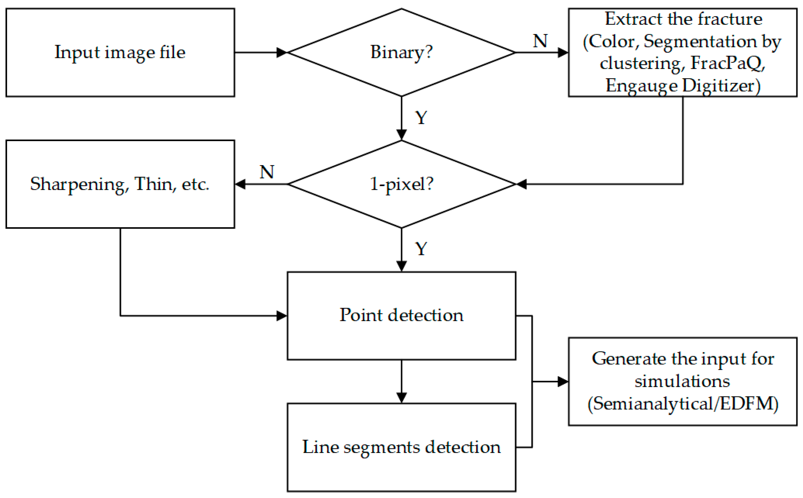
Three main steps are used in our study to detect and quantify the fracture networks. First, using fracture figures as input, the fracture endpoints and intersections are detected by point detection algorithms. Second, using these points and the original figure, fracture lines are determined and quantified. Third, the fracture length and flow orientation are computed using fracture endpoints. In this section, the methodologies of these three steps are explained one by one.
2.1. Pre-Processing
The point detection algorithms designed in this study concentrates on 1-pixel figures. In real applications, the input figures could be multi-pixels, in which case the well-established clustering algorithms and sharpening/thinning algorithms are used first to convert the original figures to a 1-pixel format. Robust clustering and sharpening algorithms are provided in many existing software such as Matlab (R2017b) for convenient use. In this study, for the simplicity of our discussion, we will assume the input figures are already in a 1-pixel format.
2.2. Points Detection
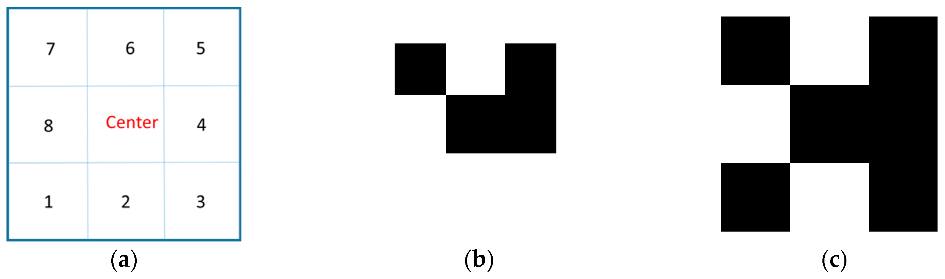
After the figures are converted to a 1-pixel format, all endpoints and intersection points need to be detected. In the 1-pixel format, each node is a cell with the 1-pixel side length and has at most 8 neighbor cells. To easily distinguish cells, the neighborhood relation for each cell is converted to a neighborhood index by assuming a binary format neighborhood relation. The bit locations used in this study are illustrated in
Figure 1a, with the target cell locating at the center. Based on this definition, the neighborhood index for each cell could only have 256 possible values, from 0–255. In fact, the neighborhood connection type is calculated using the following equation:
Figure 1b,c show two examples for this conversion. In
Figure 1b, the neighborhood index will be calculated as
, because it has neighbor cells on bit locations 4, 5, and 7. Similarly, the connection type in
Figure 1c is calculated as
since it has neighbor cells on bit locations 1, 3, 4, 5, and 7. After this conversion, all dots in the figure are converted to integer values within the range of 1 to 256 and each number is distinguishable for different neighborhood relations. With this conversion, the end points and intersection points could easily be detected out. For example, the endpoints will be dots with only one neighbor, thus there are only 8 possible values if one point is the endpoint, that is,
. When the corresponding neighborhood index equals to one of these 8 values, it will be marked as endpoints. And similarly, the intersection points are points with more than 3 neighbor dots, such as the center cell in
Figure 1b.
Using this conversion technique, all special points (endpoints and intersection points) will be detected and stored for further use in the next step.
2.3. Line Segments Detection
After locating all the special points, we proceed to the detection of the line segments. There are many line segments detecting software based on the classic method of Hough transform to recognize line segments patterns from complicated colored images. These techniques are also utilized in software like FraqPac [
26] to decide the geometry of fractures from geology photos. However, in this study, we focus on the detection of fracture segments from the input of 1-pixle format images, which are based on the endpoints and intersections detected as described in the previous section. We aim at getting an output file including the description of each fracture segment with coordinates of its start and end points, length, slope, mid points, and the connection relationship and relative connection relationships with the well, which is used as an input for the semianalytical model and numerical methods with EDFM implemented. Hence, instead of the Hough transform based methods, we propose a more intuitive but efficient way to detect the fracture segments from 1-pixel images.
2.3.1. Detection of Line Segments with Known Endpoints: Basic Idea
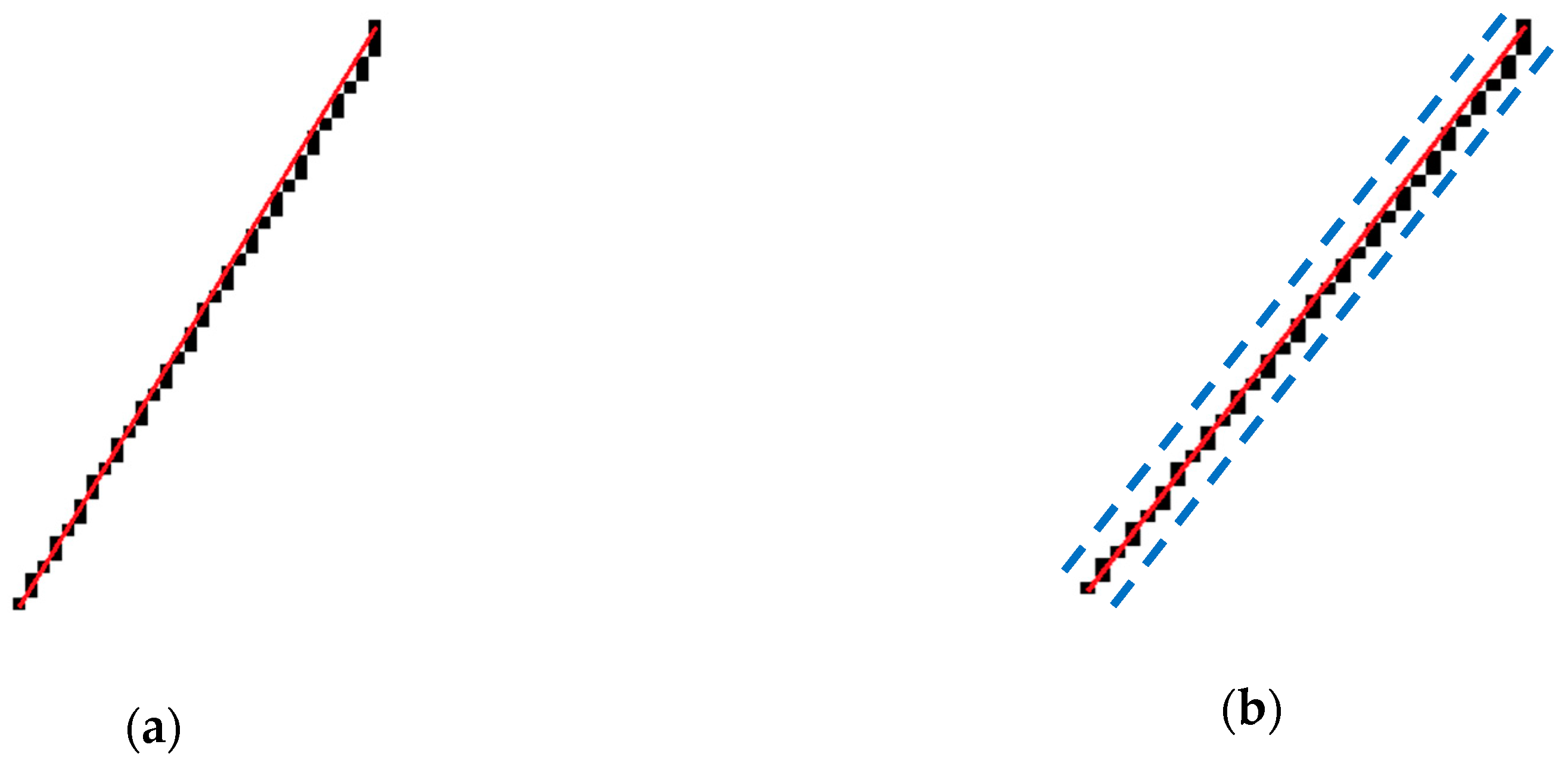
First, we describe the procedure of testing whether there is a line segment existing between two known points. With the coordinates of two points, an equation of a straight line that connects them can be directly derived. Coordinates of all the possible points on this straight line in the binary image can also be computed. As shown in
Figure 2a, due to 1-pixel image assumption, sometimes the lines on the binary image may not be perfectly straight (black connected cells), thus the point detection algorithm might lead to a straight line not perfectly passing the black cells. Hence, besides the computed points on the 1-pixel line, we should also include neighborhood points (the region within the dashed blue lines) in
Figure 2b.
Define the set of all the black points on the binary image as and the set of the computed possible points as and suppose they contain and elements, respectively. The points in on the binary 1-pixel image are determined by considering the intersection and suppose it contains elements. Consider the ratio between two sets, , if is larger than a chosen criterion (90% for the cases in this study), we mark it as a line segment. Using this method, all existing line segments could be detected. The 90% value is found by trial and errors among all the values ranging from 0 to 1. For different cases, this value might be different and should be modified accordingly to achieve the best detection results. The larger this value is, the less line segments will be detected and vice versa. For example, in the extreme case of being 100%, only the lines with all the pixels in this range will be detected, which is in some cases hard to achieve.
A disadvantage of this method should be pointed out. When there are two very close parallel fractures, it is hard to distinguish between these two tight parallel fractures using this method. At that time, the detection accuracy would decrease significantly.
2.3.2. Detection of the Lines with Endpoints and Intersections
As explained in
Section 2.2, all the end points on the fracture image can be detected first. Intuitively, with the method introduced in
Section 2.3.1, we can iterate through all the end points and decide the existence of line segments between any pair of the end points. By comparing slope and length (equivalently radius and angles) of lines starting from the same point, we can simply exclude all the repeated lines. A large number of micro-seismic data at one location is usually related to the larger aperture of that fracture or a large number of fractures in that location. In that case, a large number of fracture segments could be detected and quantified. In this study, one fracture segment is simply used to represent all possible fractures and more sophisticated cases will be studied in the future.
However, it should be pointed out that a large error exists when an image with a complex fracture structure is processed with this method. The preprocessing error of the image (especially the “sharp/thin” operation) may bring distortion to the straight lines, which will affect the detection of the intersection points. However, it is noticed from our numerical experiments that the endpoints can usually be detected correctly. Hence when the original image has a complicated fracture formation, the line segments can be detected using another method. First, the endpoints are detected, which only has negligible errors. Then we detect the line segments between these endpoints, using the technique introduced in
Section 2.3.1. In fact, the result of this step already has enough for the simulation with the EDFM method. While semianalytical methods require more information for the fracture lines, for example, the intersections of these line segments, which constitute all the points needed for the semianalytical method. In this way, the complex images such as Case 2 analyzed in
Section 3 can be processed accurately. The intersection points may not be marked in the exact position but we can get a good approximation to simulate fracture structure from a complicated image, with acceptable errors.
After line detection is finished, the angles and lengths of the fractures could be calculated using the fracture lines with the endpoints and stored for the use of the semianalytical method.
2.4. Flow Direction Determination for the Semianalytical Model
For the semianalytical method, extra fracture analysis work should be done. As shown later in the application, the semianalytical method needs the flow direction between two end points of the fractures. Our computation for flow directions is based on the relative connective relationship of each point to the wellbore.
To achieve this purpose, the shortest path problem needs to be solved, defined as finding the shortest path from each node to the wellbore. The fracture structure can be viewed as an undirected graph [
29], by regarding all the points as the nodes, and all the fracture segments as the edges. We assign each edge with the same unit weight, then by solving the shortest path problem from each point to the wellbore, we can find the distances from the points to its closest connected wellbore. The flow direction between the two points is defined by these distances. Specifically, in the models investigated in this study, because the same fracture aperture is utilized for all the fractures, for a pair of connected nodes, our assumption is that flow goes from the point with a larger distance to the well to the point of smaller distance. For the output file, all the points can also be sorted according to the distance. When fractures have different apertures, this assumption will not hold any more [
30].
In summary, the workflow for our method described in
Section 2 is illustrated in
Figure 3. Next, our technique will be applied for three unconventional reservoir cases in
Section 3.
3. Application
With the help of horizontal wells drilling and hydraulic fracturing techniques, unconventional plays have become a revolution for the energy industry since the late 1980s. In unconventional reservoirs, fractures modeling is an inevitable procedure, in which the fracture quantification needs to be done beforehand in order to simulate the fractures. The input data for fracture quantification might be micro-seismic data, fracture outcrop figures, or other information. Applying the fracture detection and quantification proposed above, the fracture information can be extracted for different reservoir simulation methods.
Efficient simulation methods of modeling fractured reservoirs include analytical methods, semianalytical methods [
6,
8,
27], and numerical methods [
31,
32]. The dual-porosity/dual-permeability approach is also often applied to model complex fractures and simulate the effect of fracture networks. However, the resolution of these approaches is not enough to capture the details of fractures.
In this section, a semianalytical method and a numerical method with EDFM implemented will be used to model the shale gas productions in the fractured reservoirs. The technique proposed in this study will be applied in three cases to show its effectiveness. The first two cases use micro-seismic data as input and the third case uses the natural fracture outcrop. After the fracture image is processed and fracture data is quantified, two reservoir simulation methods will be used to simulate the reservoir. One is a semianalytical model and the other uses a numerical method with EDFM implemented. More details of these two methods will be explained next.
3.1. Semianalytical Model
Assume the reservoir matrix is homogeneous, there are many analytical and semianalytical models dedicated to efficiently simulating the gas transport in shales. Gringarten et al. [
33] used source and Green’s functions to solve unsteady flow problems for a wide variety of reservoir flow problems. Cinco-Lay and Samaniego [
34] presented a new technique for analyzing pressure transient data for wells intercepted by a finite conductivity vertical fracture. Wan and Aziz [
35] proposed a new semianalytical solution for horizontal wells with multiple fractures with different strike angles and partially penetrating the formation in the vertical direction. Then the authors calculated the well index combined with a numerically computed gridblock pressure. Lin and Zhu [
36] studied the well performance for fractured horizontal wells in an infinite slab reservoir, by using the instantaneous solution of plane sources, in which the fractures could be fully or partially penetrated. Zhou et al. [
27] designed a semianalytical model to simulate the gas production in Barnett shale with fully penetrated planar fractures. Yu et al. [
8] extended Zhou’s model to simulate well production for reservoirs with fully a penetrated non-planar fracture as well as a planar fracture with varying fracture width and fracture permeability. Their model was verified with a numerical reservoir simulator for a single fracture case before being applied to several case studies based on Marcellus shale properties. In this section, the model built in Yu et al. [
8] is used to simulate the shale gas reservoirs.
3.2. EDFM Method
As one of the conventional methods for fracture modeling, dual-porosity/dual-permeability approaches are often applied to model complex fractures and simulate the effect of fracture networks. However, the resolution of these solutions is not high enough to capture the details of fractures geometry. To solve that issue, discrete-fracture models (DFM), using finite-volume or finite-difference methods, have been developed. To be compatible with the complex geometries of fractures, such as nonplanar fractures and fractures with variable aperture, unstructured grids-based reservoir simulator are also developed [
31,
37,
38,
39,
40] in order to explicitly model the fractures. However, the use of unstructured grids leads to high computational cost and they are still limited in real field studies. As a solution, the EDFM was developed [
3,
5,
41,
42] to honor the accuracy of DFMs while keeping the efficiency offered by structured gridding. In this study, a numerical method with EDFM implemented by Shakiba and Sepehrnoori [
28] is used to compute the pressure distributions. Due to the very small matrix permeability, pressure diffusion is very slow in the matrix, as it is apparent in the figures below. This can imply some numerical errors in the EDFM method because of the singular behavior in
of pressure close to a fracture is badly captured. In these cases, the MINC (Multiple Interacting Continua) methods for capturing short time behavior can be applied [
43,
44].
3.3. Case Study
Case 1. Vertical Barnett Shale Well
The first example comes from Fisher et al. [
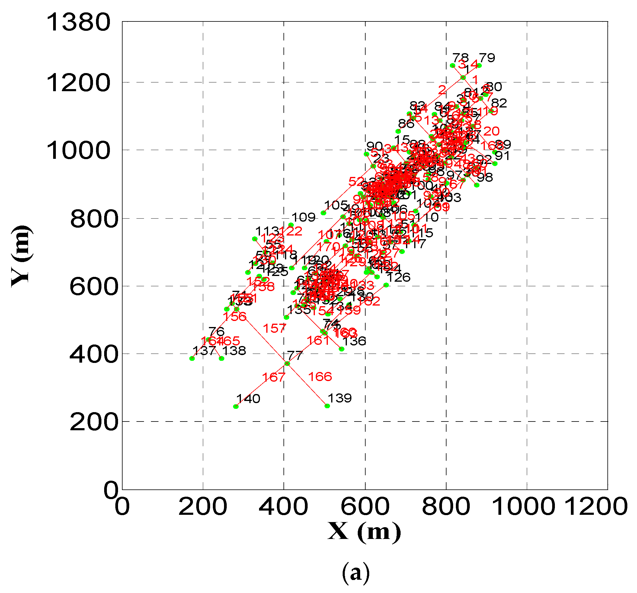
45], where the micro-seismic mapping data and conjectured fracture network in this area are given, with one active vertical well. Previously, if engineers want to use this fracture pattern, a tedious and time-consuming fracture quantification process needs to be taken, during which the researchers need to manually locate the fracture lines and endpoints. With the method proposed in this study, the only work needed to do is to set up the color of the fractures in
Figure 4a. By using clustering and sharpening methods provided by Matlab, we can get the fracture lines in binary 1-pixel format. The methods introduced in
Section 2 could then be applied to read the nodes and detect the fracture lines. The nodes and lines results are shown in
Figure 4a.
Using the nodes and line segments information provided in
Figure 4a, a semianalytical method is used to calculate the pressure distributions. The reservoir information and other properties are listed in
Table 1. The pressure profiles after 3 years and 10 years are plotted in
Figure 4b,c respectively. The stimulated rock volume could be identified from this pressure results.
Figure 4a illustrates accurate detection result of all the fractures. This case is a good example of the convenience of the auto detection workflow compared to manually locating the lines and nodes. In this case, there are over 170 fracture segments, it will be time-consuming to manually locate all the 340 plus fracture end nodes. With the help of our algorithm, it just takes several seconds to detect all the nodes and fracture segments.
Figure 4b,c show a high resolution pressure profile after 3 years and 10 years, respectively. In the top right corner, where the density of fractures is high, the pressure diffuses much faster than the bottom left corner, where there are only a few coarse fractures. This validates the important role of natural fractures in altering the shale gas flow transport mechanisms.
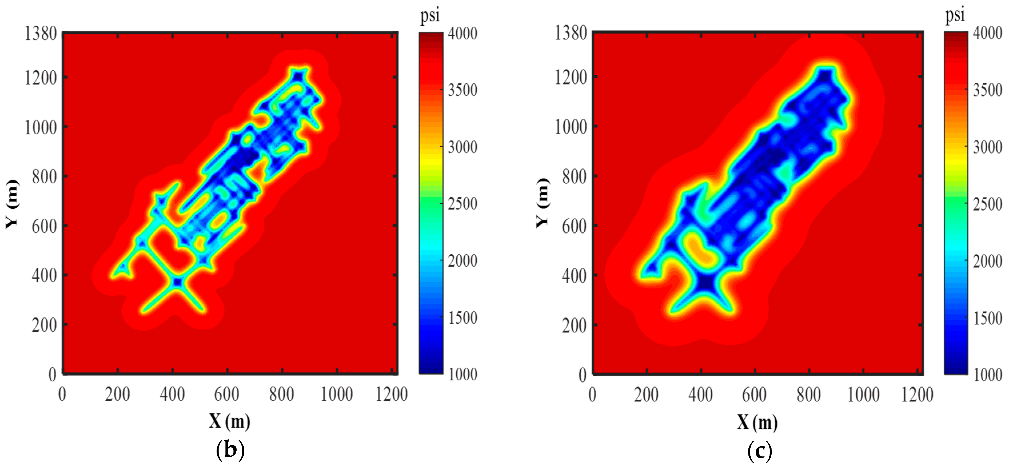
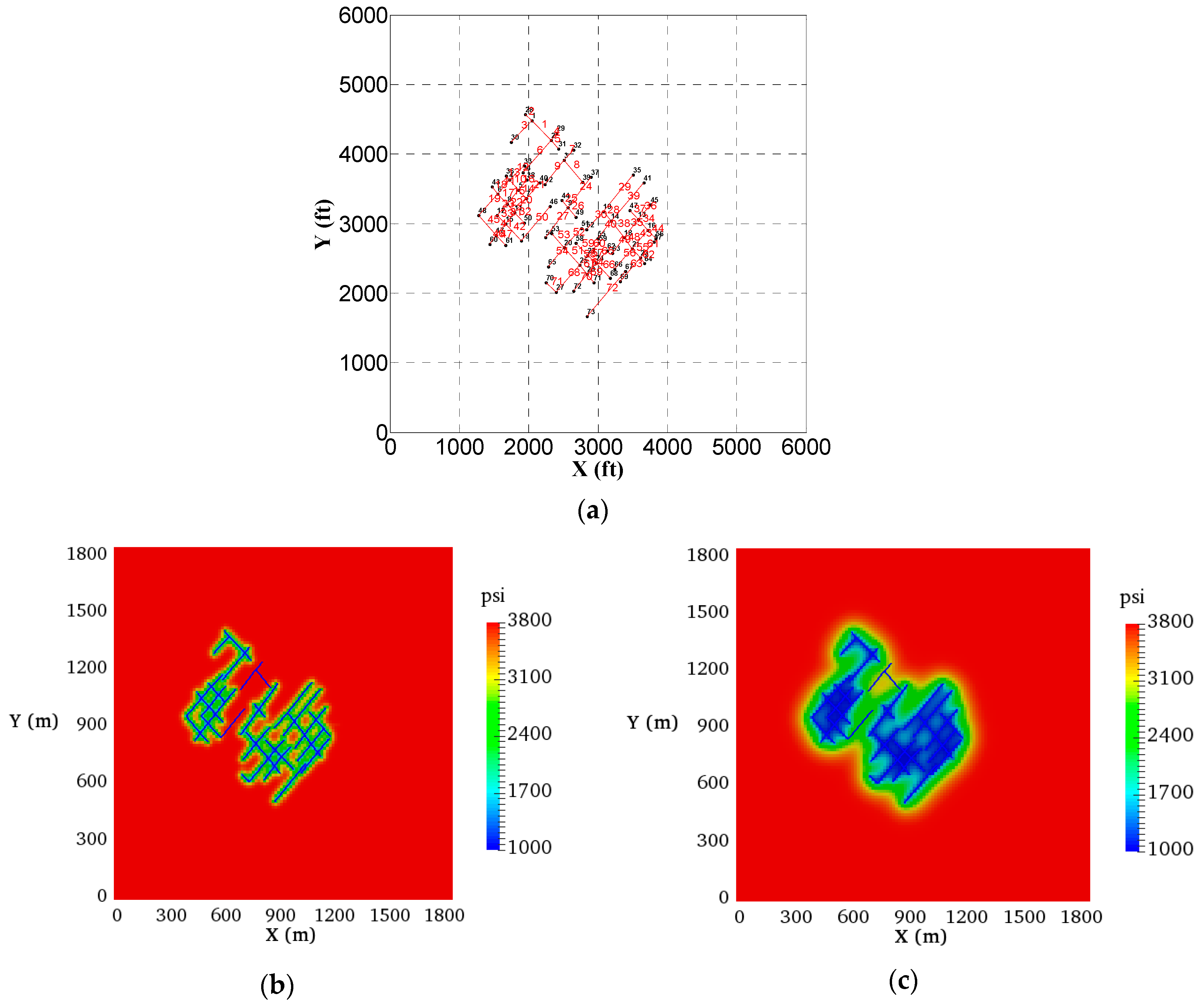
Case 2. Horizontal Barnett Shale Well
The second case is also in Barnett shale [
45] but with a horizontal well. Applying the methods introduced in this study, the nodes and line segments are detected in
Figure 5a. The Reservoir dimensions and other information is listed in
Table 2. It is a shale gas reservoir of 1829 m × 1829 m × 91 m large, with 120 × 120 × 1 mesh dimension.
Applying the fracture detection workflow introduced in this study, the fracture segments are quantified and illustrated in
Figure 5a, with nodes in black colors and line segments in red colors, the unit is still ft to make the readers easy to compare with the original fracture figure of reference [
45]. Because this case has relatively simple fracture patterns, our detection workflow gets perfect detection of all fracture segments.
Using the fracture patterns detected in
Figure 5a and the horizontal well location as shown in yellow in the figure, an in-house shale gas reservoir simulator with EDFM methods implemented is used to run the reservoir simulation. The parameters are listed in
Table 2.
After 3 years and 30 years, the pressure profile is plotted in
Figure 5b,c, respectively. Again, the pressure diffuses much faster in the high-density areas at the left part and the bottom right part. The pressure diffuses much slower in the top part because there are only four fractures.
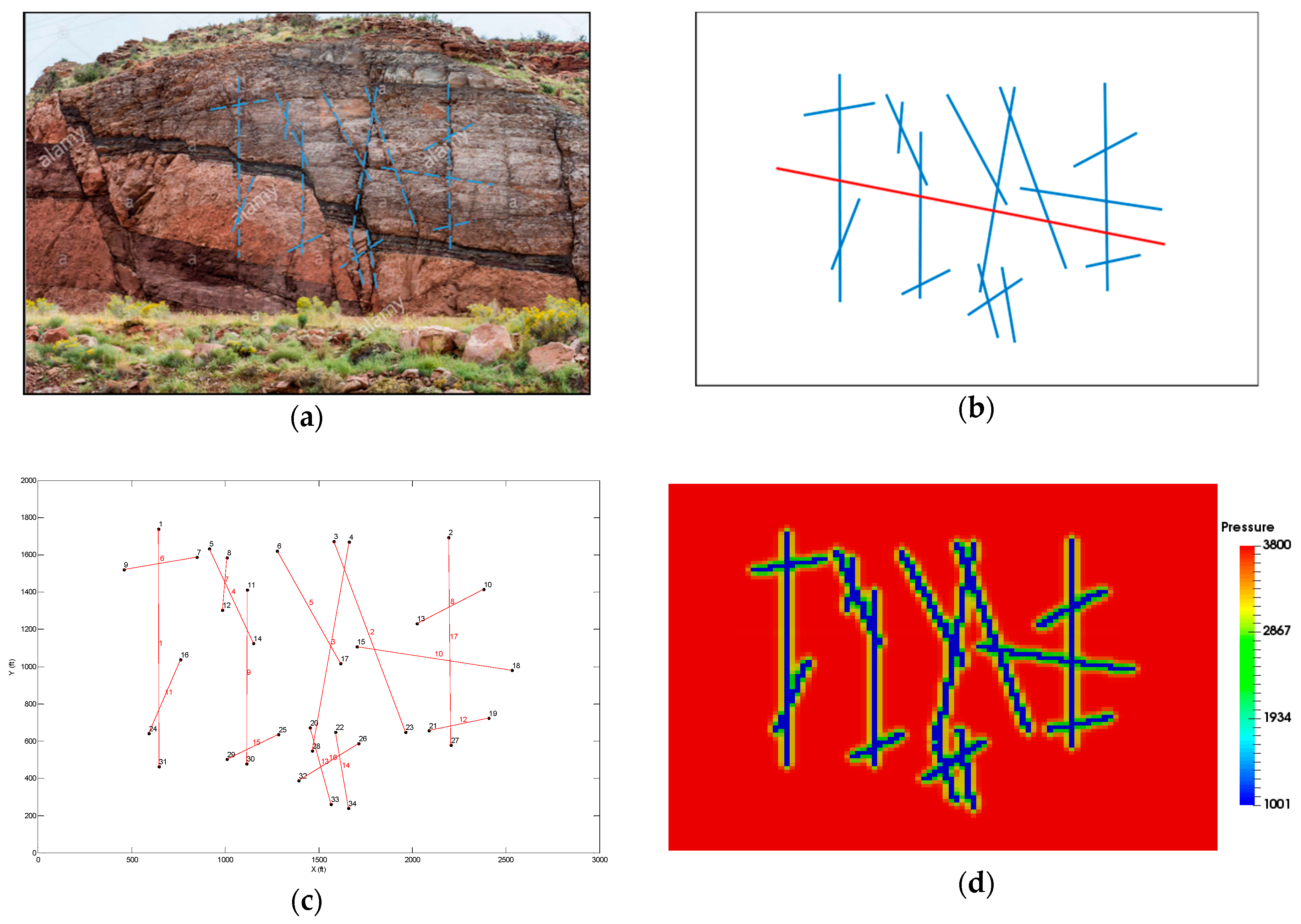
Case 3. Actual Fracture Outcrop Case (EDFM Method)
To show the versatility of our method, in the last case, an original fracture outcrop figure is used to get the fracture information. The fracture lines are drawn manually as in
Figure 6b, which is used as the input for our method and the nodes, line segments results are plotted in
Figure 6c. Here we only detect the endpoints and line segments, which are enough for the EDFM method inputs. Using the reservoir parameters as listed in
Table 3, with different dimensions, the pressure result in 3 years is shown in
Figure 6d.
Due to the limitation of our clustering algorithm, the fracture lines in
Figure 6a are still drawn manually but the fracture nodes and lines are detected based on
Figure 6b using the workflow of this study.
Figure 6c has the perfect match of all the fracture segments and nodes. Using the fracture information shown in
Figure 6c, our in-house reservoir simulator with EDFM method implemented is used to run the simulation for 3 years. The pressure result (in psi) is shown in
Figure 6d.
5. Discussion
Fracture quantification and modeling are an inevitable procedure in an unconventional reservoir simulation. Accurate fracture quantification could build a strong foundation for fracture modeling because fractures could largely impact the fluid transport mechanism in unconventional reservoirs. In this study, using two-dimensional fracture figures as input, a fracture detection, and modeling workflow is proposed to quantify the fracture networks in fractured reservoirs.
Using clustering algorithms, two-dimensional fracture figures could be converted to a binary 1-pixel format. The connection types of all the fracture nodes are converted to integers in order to detect the end points and intersection points of fracture segments. Then the fracture segments are detected by checking the overlaps between existing nodes between two points and the lines connecting two points to see whether the overlap ratio is higher than 90%, the line segment is accepted. For semianalytical methods of reservoir simulation, the extra shortest distance problem needs to be solved to get the flow direction in any fracture segment. The fracture information computed by this method provides all the necessary input data for fracture modeling in semianalytical methods and EDFM methods. To validate our model, three reservoir cases are constructed using either the micro-seismic data or the field fracture outcrop data, before the semianalytical method and a numerical method with EDFM implemented are used to simulate the reservoir model and compute the pressure profiles.
To the best of the authors’ knowledge, this work is the first work of applying image processing techniques to directly quantify fracture patterns for fracture modeling in unconventional reservoirs. Due to the complexity of the fracture networks, the detection accuracy is not 100% for some complicated fracture patterns, which will be further improved by refining our clustering techniques.
On the other hand, because this study concentrates on the fracture segments detection, the input data is assumed to be the binary and 1-pixel format in the 2D plane. However, in practical cases, there are only the original JPEG format figures and they are in 3D space. In the future, with more advancement in machine learning and clustering and with the help of advanced image processing algorithms to handle the clustering work, original multi-pixel colored figures can be accepted as input. It is also possible to reconstruct some 3D fracture models having mainly observed 2D traces as well as well data, in which the hydraulic fractures are likely to be 2D planar objects that intersect natural fractures along some segments. Some techniques have been proposed to model transient fluid flows in 3D DFN by mapping the fractures to an equivalent pipe network [
47,
48]. The resulting problem is similar to the one got using EDFM methods or others. Meanwhile, multiphase flow can also be addressed using the mixing of dual porosity models and streamlines models [
49,
50,
51]. In the future, more field cases will be studied with these advanced techniques.
Despite the above limitations, the methods proposed in this work could inspire further applications of image processing in the energy field, especially in the oil and gas industry. Image processing ability is a must capacity for future exploration robots or equipment. It is worthwhile to put more effort into this area, in order to get ready for assembling the first automated exploration subsurface robot and further propel the development of the oil and gas industry.


