District Power-To-Heat/Cool Complemented by Sewage Heat Recovery

Abstract

District heating and cooling (DHC), when combined with waste or renewable energy sources, is an environmentally sound alternative to individual heating and cooling systems in buildings. In this work, the theoretical energy and economic performances of a DHC network complemented by compression heat pump and sewage heat exchanger are assessed through dynamic, year-round energy simulations. The proposed system comprises also a water storage and a PV plant. The study stems from the operational experience on a DHC network in Budapest, in which a new sewage heat recovery system is in place and provided the experimental base for assessing main operational parameters of the sewage heat exchanger, like effectiveness, parasitic energy consumption and impact of cleaning. The energy and economic potential is explored for a commercial district in Italy. It is found that the overall seasonal COP and EER are 3.10 and 3.64, while the seasonal COP and EER of the heat pump alone achieve 3.74 and 4.03, respectively. The economic feasibility is investigated by means of the levelized cost of heating and cooling (LCOHC). With an overall LCOHC between 79.1 and 89.9 €/MWh, the proposed system can be an attractive solution with respect to individual heat pumps.

1. Introduction

District heating and cooling (DHC) is considered more efficient than individual, distributed systems for heating and cooling, especially because DHC solutions can benefit from locally available, low-cost energy sources, like environmental heat and cool, industrial waste heat and solid waste incineration [1], but DHC, as a heat/cool demand aggregator with thermal storage capacity, can offer also flexibility in managing energy demand. In the future power grid dominated by renewable non-programmable electricity, this feature would contribute to make DHC solutions based on power-to-heat/cool technologies of strategic importance [2]. Existing DHC systems using large size, electricity driven heat pumps are examples in this field. These systems can provide social and environmental benefits when used to replace heating technologies relying on combustion in densely populated urban areas, where air pollution is an impelling problem. Concerning heat pump technologies, different low-grade heat sources have been used in existing district heating (DH) plants, including industrial excess heat, ambient water and sewage water. Sewage water is widely adopted in Sweden, where DH plants utilizing sewage water represents about 50% of the heat generated by power-to-heat DH plants [3]. Regarding power-to-cool conversion, examples of large DHC systems have been proposed in Japan [4], in which river water constituted the most efficient heat sink.

Wastewater heat recovery applications based on heat pumps are becoming widespread in energy saving applications for both heating and cooling. Heat recovery can be performed inside the buildings (domestic), from sewerage lines (urban) and from wastewater treatment plants (municipal). In the review conducted in [5], COP values in the range of 1.77–10.63 for heating and 2.23–5.35 for cooling are reported based on the experimental and simulated values. Moreover, the sewage heat exchanger is one of the key components in wastewater-source heat pumps. Different types of sewage heat exchangers have been used, including shell & tube, plate, spiral, gravity-film and channel type [6]. In domestic utilization, a consistent amount of heat energy can be recovered from washers, dishwashers and showers. Gravity film and spiral heat exchangers can be used directly in the drainage system. In wastewater heat recovery at urban scale, both channel type and external (e.g. shall & tube, plate) heat exchangers are used. External heat exchangers are more effective although they require wastewater screening and extra pumping and piping system. The heat recovery at municipal scale is technically easier, although water treatment plants are seldom close to the consumer.

In densely populated areas, heat recovery from sewage at urban scale has a large potential, as shown in [7] where, through a GIS-based analysis that matched availability of sewage and heat demand, high utilization factors of the heat theoretically recoverable at the final treatment plant are found for different sewerage lines in Tokyo. However, untreated urban sewage is not widely used due to the problem of filth. Auto-avoiding-clogging equipment can be used to continuously capture suspended solids in the sewage as in [8], where an untreated sewage source heat pump (USSHP) system is experimentally investigated showing COP of the heat pump unit and of the system of 4.3 and 3.6, respectively. The operational experience with another type of filth block device is reported in [9], where an urban sewage source heat pump system composed of a filth block device, a wastewater heat exchanger, and a heat pump is demonstrated. The results indicated that in typical conditions the heating COP is about 4.3 and the cooling COP is about 3.5.

Based on these premises, the energy and economic feasibility of a DHC system based on a large size heat pump and complemented by sewage heat/cool recovery is investigated. The system is conceived to alternatively supply heat and cool to a commercial district located in northern Italy, a densely populated area where air quality is a main concern and commercial buildings, characterized by heating and cooling loads of comparable magnitude (respectively about 100 kWh/m² year and 75 kWh/m² year [10,11]), highly contribute to the local thermal energy demand and the associated emissions of air pollutants. Communal sewage provides the heat source in heating and the heat sink in cooling. With respect to sewage potential and availability, it is worth noticing that Italy is characterized by a large per capita water consumption, 175 liter/day/person [12]. Such a system would offer the following main advantages: (1) ability to exploit the increasing share of renewable electricity in the electricity mix, which implies lower CO₂ emissions as compared to gas boilers for heating; (2) ability to purchase electricity on the wholesale market at competitive tariffs, as compared to the average electricity consumer; (3) zero local emissions of air pollutants (e.g., PM, NOx), as compared to gas boilers and DH conversion systems relying on combustion (e.g., CHP); (4) possibility to exploit PV electricity generated on-site by a large capacity PV plant that can benefit from economies of scale. The analysis aims to estimate the overall plant efficiency, including heat losses and parasitic energy consumption, and the economic competitiveness and the environmental benefit as compared to individual electrical heat pumps, which represent an alternative of comparable social and environmental impact for the location considered. To answer these questions, a detailed mathematical model of the system is built and simulated in Trnsys [13].

2. Plant Configuration and Operation

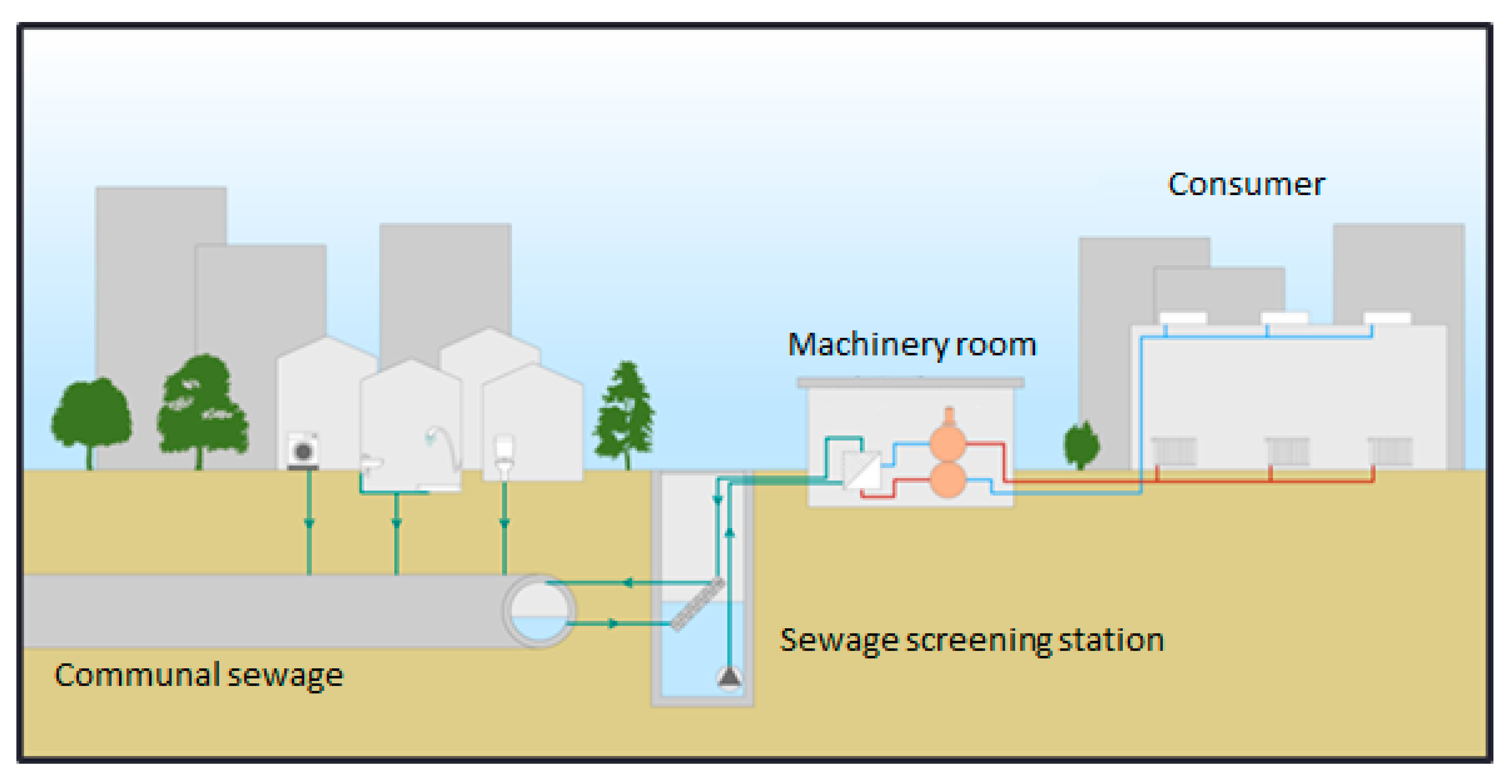
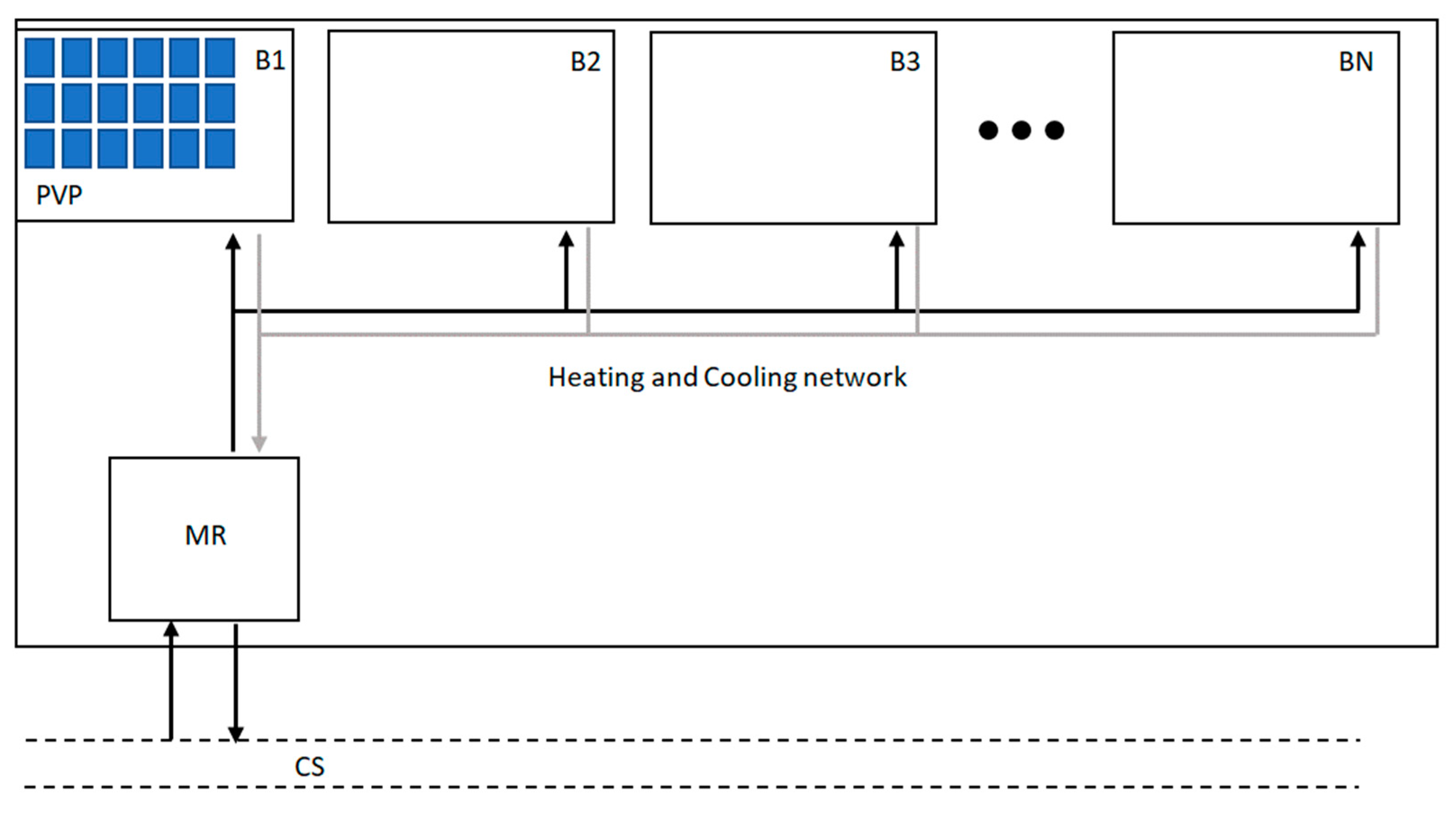
The general scheme of a district heating and cooling system using sewage heat recovery is displayed in Figure 1. Communal sewage is accessible at relatively close distance from the thermal energy consumer. After screening, sewage exchanges heat with a vapor compression heat pump, located in the machinery room, that supplies thermal energy to the consumer through a heating and cooling network.

In the plant configuration considered within this work, the DHC network supplies heat, in winter, and cool, in summer, to a commercial district comprising distinct department stores. The seasonal switch from heating to cooling occurs typically at end of April and the cooling season lasts until mid-October. Due to the simultaneity of the thermal demand across buildings of similar characteristics, a two-pipe network is used. At the end-user, hot water is supplied at 50 °C with a peak load temperature drop of 10 °C and chilled water at 6 °C with peak rise of 7 °C. PV panels are installed on a portion of the overall flat surface available on buildings roofs (see Figure 2).

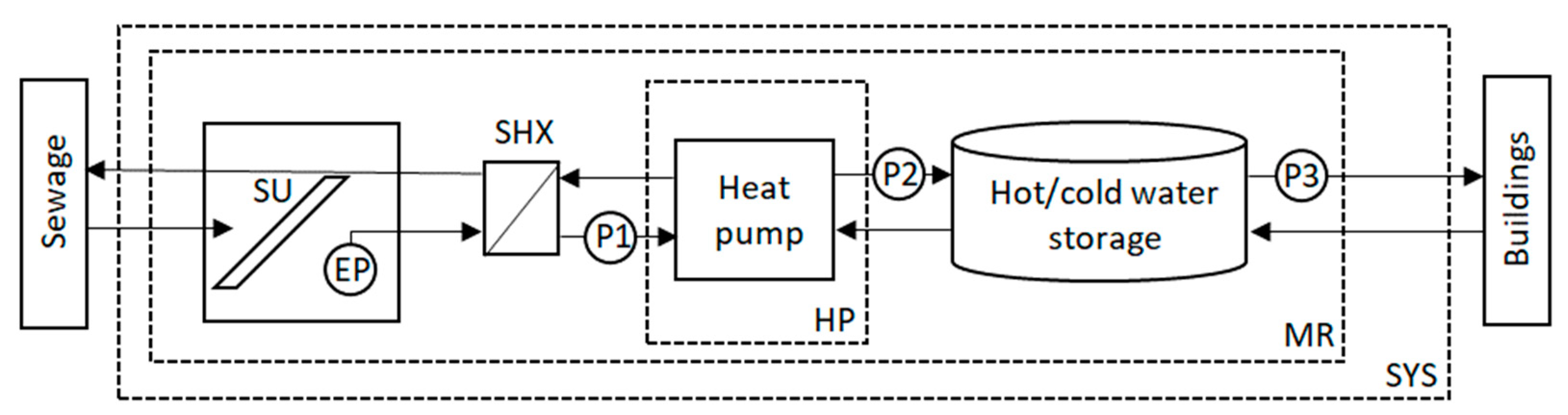
The machinery room (see Figure 3), located underground, comprises sewage basin with screening unit, elevation pump, sewage heat exchanger, heat pump and hot/cold water storage. The heat pump operation mode can change from heating to cooling through inversion on the external water loops (not shown in Figure 3).

The electricity of the PV system is used to drive the system pumps and the heat pump, in conjunction with the electricity purchased from the grid. If PV electricity is generated in excess, the surplus is supplied to the electricity grid. The remuneration of the electricity supplied to the grid is determined according to the net metering regulation currently in force [14], which allows selling at a tariff constituted by the sum of the wholesale electricity price and a contribution related to the system charges and general transmission and distribution costs.

The control strategy is defined with the objective to limit parasitic energy consumption. Therefore, variable speed pumps are used. Pump P2 operates to keep the water storage at the desired set point temperature. The heat pump compressor frequency is modulated to: (i) deliver water at the desired temperature to the water storage when heat pump capacity is overabundant (partial load); (ii) limit above 0 °C the temperature of the water sent to the SHX in heating operation to prevent the evaporator from freezing (antifreeze protection); (iii) limit below 50 °C the temperature of the water sent to the SHX in cooling operation to prevent excessive heating of sewage (overheating protection). Pumps EP and P1 modulate their speed based on the compressor speed. Pump P3 is controlled according to the network return temperature, as further explained in the following section.

3. Mathematical Model

In the following, the mathematical models of the main system components are presented. The models are calibrated and validated against the manufacturer’s data of a reference unit. Their outputs, once scaled with respect to the capacity of the reference unit, are assumed representative for units slightly different in size.

3.1. Heat Pump

The heat pump model predicts condenser heat duty (${\dot{Q}}_{cond}$), evaporator heat duty (${\dot{Q}}_{evap}$) and compressor power input ($W_{comp}$) at different values of chilled water inlet temperature ($T_{cwi}$), chilled water mass flow rate (${\dot{m}}_{cw}$), hot water intel temperature ($T_{hwi}$), hot water mass flow rate (${\dot{m}}_{hw}$) and compressor frequency ($f$) by means of thermodynamic modelling. The reference unit is a screw chiller of 788 kW heating capacity using R134a as refrigerant [15]. 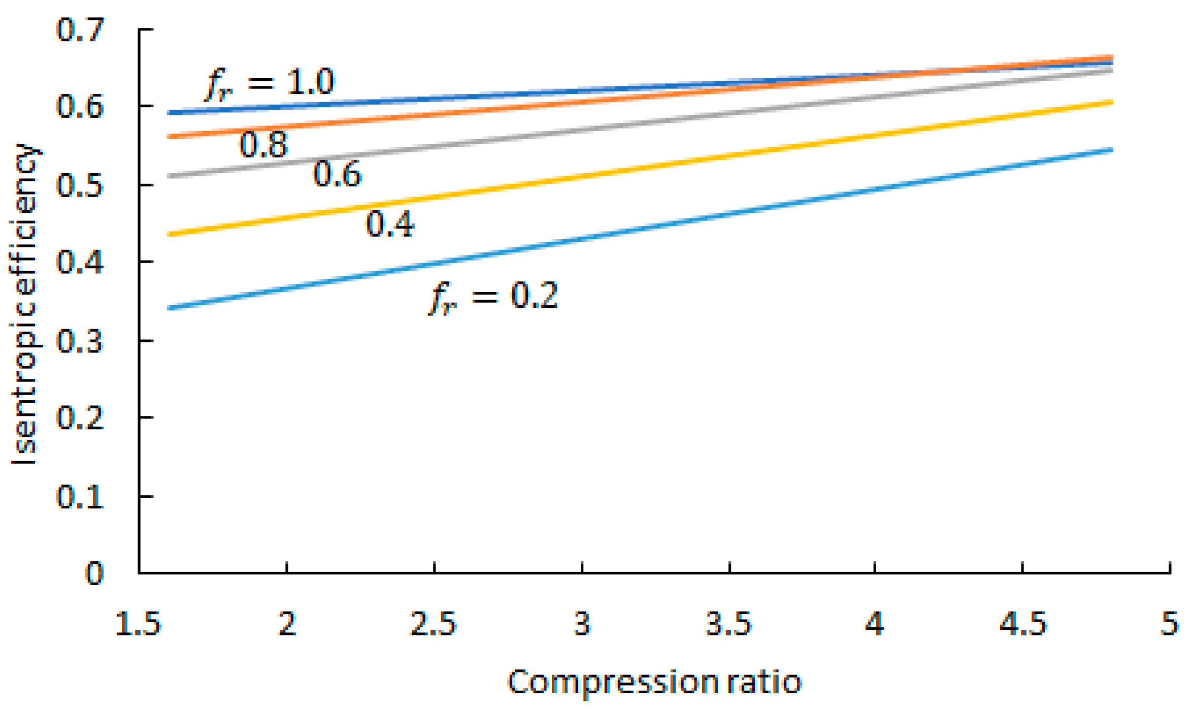Based on the refrigerant property [16], the cycle state points are determined by imposing constant temperature differences for the following temperature pairs: refrigerant condensation and hot water outlet (0 K), hot water inlet and refrigerant at condenser outlet (1 K), chilled water outlet and refrigerant evaporation (1 K), chilled water inlet and superheated vapor at evaporator outlet (1 K). Isentropic efficiency as function of compression ratio ($P_{cond}/P_{evap}$) and frequency ratio ($f_r=f/f_{nom}$) is used for calibrating the model output with the performance data derived from the manufacturer’s datasheet. The resulting functional dependency is shown in Figure 4.

Volumetric flow rate at compressor inlet is assumed proportional to frequency ratio and its maximum value (${\dot{V}}_{max}$) is calibrated based on the heat pump nominal heating capacity (${\dot{Q}}_{cond,nom}$). The resulting scale factor $s={\dot{V}}_{max} /{\dot{Q}}_{cond,nom}$ is 0.331 m³/s MW. The comparison between model output and manufacturer’s data is presented in

Table A1. Model results and manufacturer’s data in heating mode (H) and cooling mode (C).

${\mathit{T}}_{\mathit{c}\mathit{w}\mathit{i}} (°\mathbf{C})$	${\mathit{T}}_{\mathit{c}\mathit{w}\mathit{o}} (°\mathbf{C})$	${\mathit{T}}_{\mathit{h}\mathit{w}\mathit{i}} (°\mathbf{C})$	${\mathit{T}}_{\mathit{h}\mathit{w}\mathit{o}} (°\mathbf{C})$	${\dot{\mathit{m}}}_{\mathit{c}\mathit{w}} (\mathbf{kg}/\mathbf{s})$	${\dot{\mathit{m}}}_{\mathit{h}\mathit{w}} (\mathbf{kg}/\mathbf{s})$	Mode (H/C)	EER/COP Model	EER/COP Manuf.	Error (%)
12.0	7.0	50.0	60.0	28.2	19.1	H	3.62	3.64	−0.6
13.0	9.3	52.5	60.0	28.2	19.1	H	3.7	3.56	3.9
14.0	11.5	55.0	60.0	28.2	19.1	H	3.48	3.43	1.4
15.0	13.8	57.5	60.0	28.2	19.1	H	3.05	3.14	−2.7
12.0	7.0	30.0	35.0	34.6	41.0	C	5.24	5.09	3
10.7	7.0	26.0	29.7	34.6	41.0	C	6.36	5.98	6.4
9.5	7.0	22.0	24.4	34.6	41.0	C	6.89	6.77	1.7
8.2	6.0	18.0	20.2	34.6	41.0	C	5.68	5.84	−2.9

, showing very good accuracy in different operating conditions.

3.2. Sewage Heat Exchanger

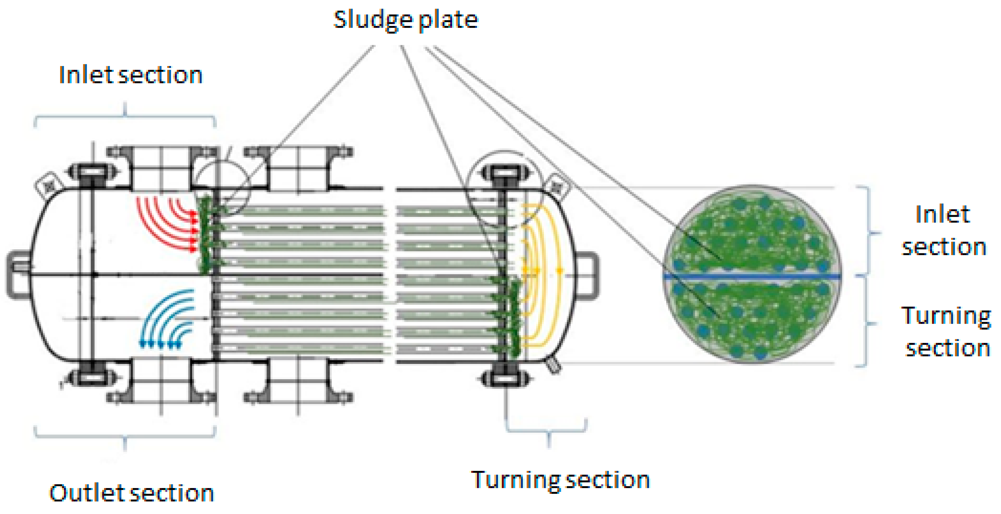
The sewage heat exchanger (SHX) comprises screening unit, elevation pump, and shell and tube heat exchanger. Sewage circulates in the tubes and clean technical water flows inside the shell, in a counterflow arrangement (see Figure 5). Concerning the parasitic energy consumption of the SHX, sewage elevation is the main cost. As the partial load value in the simulations is generally very high, the exponential dependence of the parasitic energy consumption on the sewage water flow rate is linearized. The proportionality factor ($e_{shx}$), estimated based on experimental data, is provided in

Table A2. Sewage heat exchanger model parameters.

Parameter	Value	Unit
$e_{shx}$	0.1	kWh/kg
$\tau$	260	h
$t_{cr}$	33	h
$\epsilon$	0.6	-

.

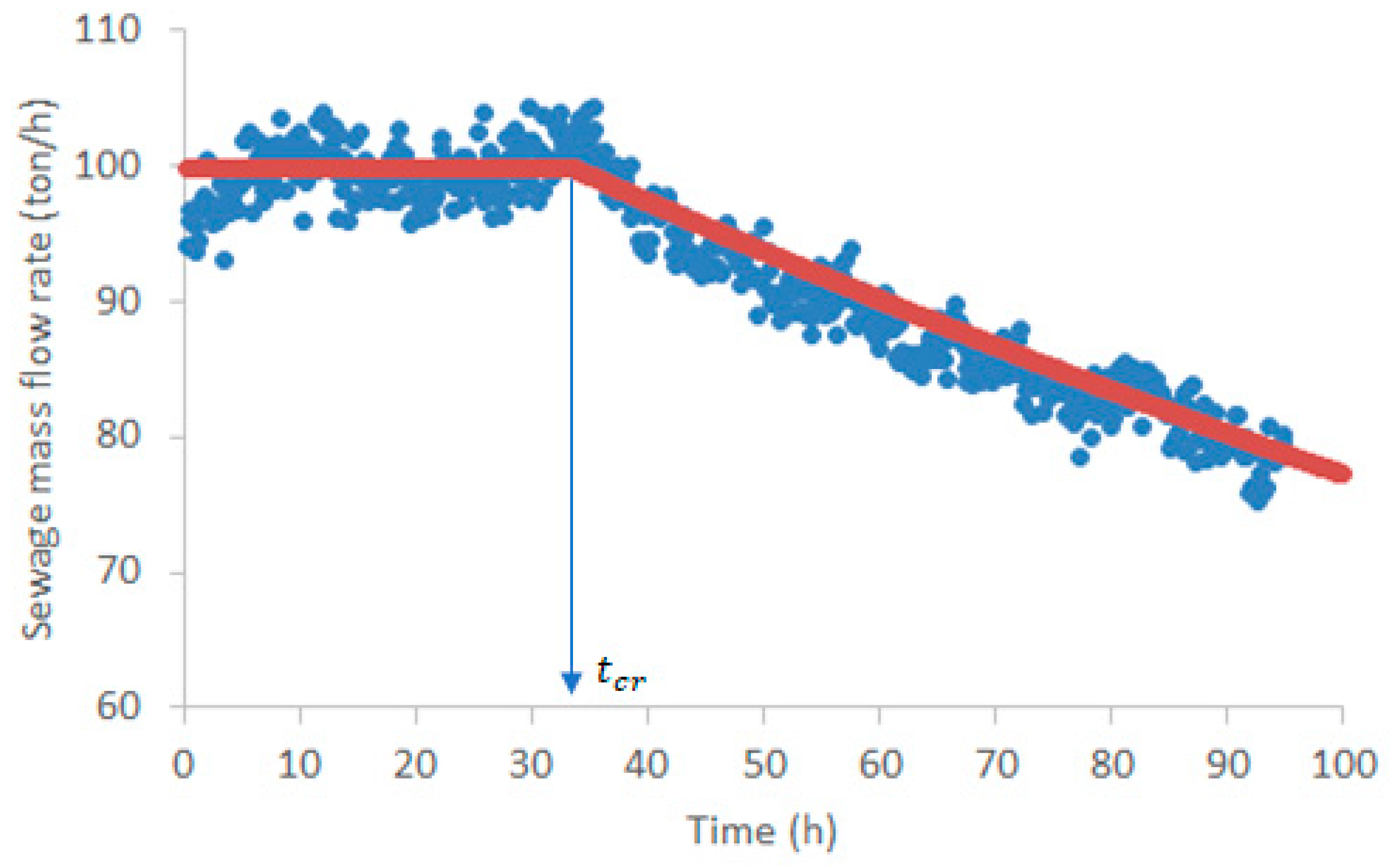
One of the main issues with the SHX is sludge accumulation at the inlet sections of the tube banks, which progressively decreases flow passage area ($S_{flow}$), sewage mass flow rate (${\dot{m}}_s$), and ultimately heat transfer rate. Cleaning is thus necessary to periodically restore the nominal performance. To calculate the influence of performance degradation, a model for the prediction of sewage flow rate is developed starting from the balance equation for the mass of sludge:

$$\frac{d{m}_a}{dt}={\dot{m}}_d-{\dot{m}}_r$$

(1)

where ${\dot{m}}_d$ is sludge deposition, ${\dot{m}}_r$ is sludge removal and $m_a$ is the mass of sludge accumulated at the entrance region of the tubes bank. According to the fouling model of Kern & Seaton [17], ${\dot{m}}_d\propto {\dot{m}}_s$ and ${\dot{m}}_r\propto {\tau }_s{m}_a$ where ${\tau }_s$ is the shear stress. With the hypothesis of (1) negligible removal, (2) constant pressure drop across inlet and outlet sections, (3) constant friction factor and (4) constant hydraulic diameter (i.e. assuming occlusion of one pipe at a time), Expression (1) can be recast as:

$$\frac{d{m}_a}{dt}=\left(\alpha \sqrt{\mathsf{\Delta }P}\right)S_{flow}$$

(2)

where $\alpha$ is a constant, $\mathsf{\Delta }P$ is the pressure drop across inlet and outlet sections, and $S_{flow}$ is the flow passage area which is equal to $S_0$ after cleaning. The reduction of $S_{flow}$ is not directly proportional to sludge accumulation because initially sludge is likely to accumulate in stagnation zones which do not contribute to flow passage area. For the derivation of an approximated empirical law, a critical sewage mass ($M_{s,cr}$), after which $-d{S}_{flow}$ becomes proportional to $d{m}_a$ through a constant proportionality factor ($\beta$), is assumed:

$$M_{s,cr}={{\displaystyle \int }}_0^{t_{cr}}{\dot{m}}_{s}dt$$

(3)

In conclusion, a differential equation for $S_{flow}$ is obtained in the form:

$$\frac{d{S}_{flow}}{dt}=-\left(\alpha \beta \sqrt{\mathsf{\Delta }P}\right)S_{flow};t>t_{cr}$$

(4)

Since under the current simplifying assumptions $\dot{m_s}\propto \sqrt{\mathsf{\Delta }P}{S}_{flow}$, the following expressions for $\dot{m_s}$ can be derived:

$${\dot{m}}_s={\dot{m}}_{s,0};0\le t<t_{cr}$$

(5)

$${\dot{m}}_s={\dot{m}}_{s,0}{e}^{-\frac{\mathsf{\Delta }t}{\tau }};t_{cr}\le t<\infty$$

(6)

where $t_{cr}$ and $\tau =1/\left(\alpha \beta \sqrt{\mathsf{\Delta }P}\right)$ are identified experimentally (see Figure 6) and their values are provided in Table A2.

The result can be generalized to the case of variable pressure drop, assuming constancy of pressure drop during a timestep interval [$\left(i-1\right)\mathsf{\Delta }t$; $i\mathsf{\Delta }t$]:

$${\dot{m}}_{s,i}=\left[{\dot{m}}_{s,i-1}\right]e^{-\sqrt{f_i}\mathsf{\Delta }t/\tau }$$

(7)

$${\dot{m}}_{s,i,v}=\sqrt{f_i}{\dot{m}}_{s,i}$$

(8)

where $f_i=\mathsf{\Delta }{P}_i/\mathsf{\Delta }\mathrm{P}$. Expressions (7) and (8) are easily implemented in transient simulations and allow considering variable flow control ($f_i\le 1$) and periods during which the SHX is not in operation ($f_i=0$). Lastly, the UA value of the SHX is determined from the well-known expression of $NTU\left(\epsilon ,C_r\right)$ valid for counterflow heat exchangers, with $C_r$ the fraction of the heat capacities of the media considered smaller than 1:

$$NTU=\frac{1}{C_r-1}\ln \left(\frac{\epsilon -1}{\epsilon C_r-1}\right)$$

(9)

Effectiveness ($\epsilon$) and the mass flow rates of each stream are measured in clean conditions and the corresponding UA is calculated. With the accumulation of sludge at the entrance sections, the degradation of the UA is idealized as the consequence of the decrease in effective heat transfer area resulting from the progressive blocking of the internal tubes. Therefore, it is assumed that UA is directly proportional to $S_{flow}$.

3.3. District Heating and Cooling Network

The pipeline diameter is sized according to the design volumetric flow rate and pressure drop. Since the simulation timestep (one hour) is about four/five times as large as the water transition time through the pipeline, a one-node lumped capacity model with heat losses is used for both forward and return pipes. The control law of the mass flow rate ($\dot{m}$) is based on the return temperature and assumes that load ($\dot{Q}$) is initially modulated by lowering the mass flow rate in the attempt to keep constant the temperature difference across supply and return ($\mathsf{\Delta }T$), and by lowering the $\mathsf{\Delta }T$ when mass flow rate is towards its minimum value. A suitable, arbitrary mathematical formula that reproduces the control law of $\mathsf{\Delta }T$ with $\dot{Q}$ is Expression (10), from which Expression (11) can be derived:

$$\frac{\mathsf{\Delta }T}{\mathsf{\Delta }{T}_{max}}=1-{\left(\frac{\dot{Q}}{{\dot{Q}}_{max}}-1\right)}^4$$

(10)

$$\frac{\dot{m}}{{\dot{m}}_{max}}=\frac{\mathsf{\Delta }{T}_{max}}{\mathsf{\Delta }\mathrm{T}}\left[1-{\left(1-\frac{\mathsf{\Delta }T}{\mathsf{\Delta }{T}_{max}}\right)}^{1/4}\right]$$

(11)

The parasitic consumption of the pump is estimated based on mass flow rate, hydraulic characteristic of the pipeline, and pump efficiency. The hydraulic characteristic can be estimated based on the network design parameters, whose values are presented in Section 4.3.

3.4. Heating and Cooling Loads

The district heating plant must be sized according to both heating and cooling loads, therefore suitable heating and cooling hourly profiles must be generated using a building energy model.

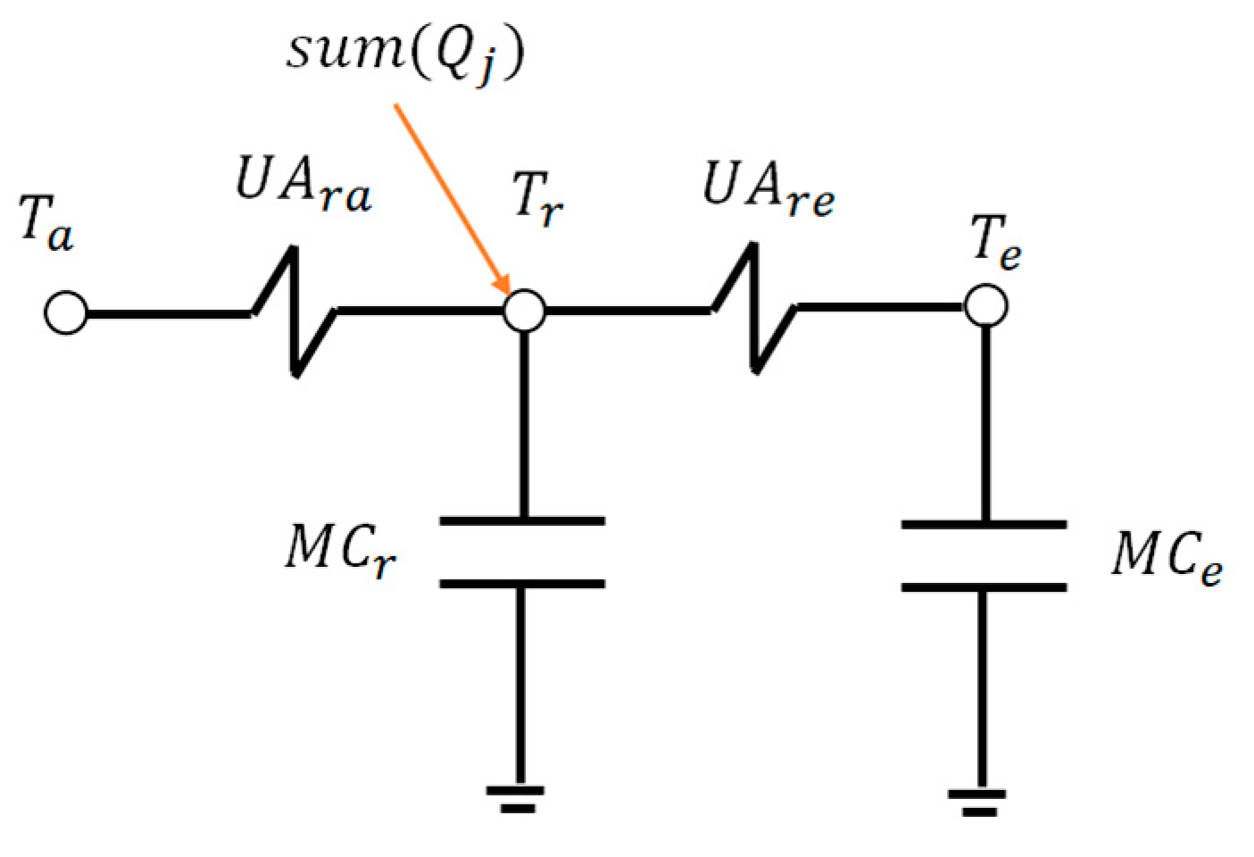
The two-node capacitive building model is shown in Figure 7, whose states are room air temperature ($T_r$) and inner building envelope temperature ($T_e$) and $T_a$ refers to the ambient temperature. Such a model is selected because as compared to more sophisticated models, it requires a minimum set of input data that can be easily tuned based on floor area, indoor volume, building envelope insulation characteristics, and target specific heating and cooling demands:

• UA between room air and outdoor ambient air ($U{A}_{ra}$, W/K)
• UA between room air and the inner building envelope ($U{A}_{re}$, W/K)
• Thermal capacity associated to the room air ($M{C}_r$, J/K)
• Thermal capacity associated to the inner building envelope ($M{C}_e$, J/K)
• Occupation density (p/m²)
• Internal gain, e.g. lights (W/m²)
• Ventilation (vol/h)
• Infiltration (vol/h)
• Fraction of solar radiation transmitted to room air (-)
• Daily comfort hours (from-to h)
• Heating and cooling daily schedule (from-to h)
• Cooling setpoint temperature (°C)
• Heating setpoint temperature (°C)

Based on outdoor ambient temperature and radiation on the horizontal plane, the model calculates solar input (${\dot{Q}}_s$), internal gain (${\dot{Q}}_i$), heat gain of the occupants (${\dot{Q}}_p$), sensible and latent heat gain of ventilation and infiltration (${\dot{Q}}_{vs}$ and ${\dot{Q}}_{vl}$), and predicts heating $({\dot{Q}}_h)$ and cooling (${\dot{Q}}_c)$ loads applying the following energy balances:

$$M{C}_r\frac{d{T}_r}{dt}={\dot{Q}}_h-{\dot{Q}}_c+{\dot{Q}}_s +{\dot{Q}}_i+{\dot{Q}}_p+{\dot{Q}}_{vs}+{\dot{Q}}_{vl}-U{A}_{ra}\left(T_r-T_a\right)$$

(12)

$$M{C}_e\frac{d{T}_e}{dt}=U{A}_{re}\left(T_r-T_e\right)$$

(13)

3.5. Key Performance Figures

The following energy and economic performance figures are introduced to evaluate the performance of the system:

(1)

Heat pump seasonal COP:

$$CO{P}_{HP}=Q_{H,HP}/E_{HP}$$

(14)

where $Q_{H,HP}$ is the cumulated heat delivered by the condenser in heating mode operation and $E_{HP}$ is the associated electrical consumption of the compressor.

(2)

Heat pump seasonal EER:

$$EE{R}_{HP}=Q_{C,HP}/E_{HP}$$

(15)

where $Q_{C,HP}$ is the cumulated cool delivered by the evaporator in heating mode operation and $E_{HP}$ is the associated electrical consumption of the compressor.

(3)

System level seasonal COP:

$$CO{P}_{SYS}=Q_{H,SYS}/\left(E_{HP}+E_{SU}+E_{P1}+E_{P2}+E_{P3}\right)$$

(16)

where $Q_{H,SYS}$ is the cumulated heat delivered to the users net of heat losses through storage and network and the denominator comprises the associated electricity consumption of the heat pump compressor $\left(E_{HP}\right)$ and all pumps ($E_{SU}$, $E_{P1}$, $E_{P2}$, $E_{P3}$).

(4)

System level seasonal EER:

$$EE{R}_{SYS}=Q_{C,SYS}/\left(E_{HP}+E_{SU}+E_{P1}+E_{P2}+E_{P3}\right)$$

(17)

where $Q_{C,SYS}$ is the cumulated cool delivered to the users net of cool losses through storage and network and the denominator comprises the associated electricity consumption of the heat pump compressor and all pumps.

(5)

Full load equivalent hours:

$$FLEH=\frac{Q_{H,SYS}}{{\dot{Q}}_{cond,nom}}+\frac{Q_{C,SYS}}{{\dot{Q}}_{evap,nom}}$$

(18)

where ${\dot{Q}}_{cond,norm}$ is the nominal power of the condenser and ${\dot{Q}}_{evap,nom}$ is the nominal power of the evaporator.

(6)

Levelized cost of heating and cooling:

$$LCOHC=\frac{CAPE{X}_a+OPEX-B}{Q_{H,SYS}+Q_{C,SYS}}$$

(19)

where $CAPE{X}_a$ is calculated for each plant component by dividing investment cost times annuity factor, function of discount rate and useful life. $OPEX$ includes maintenance costs, evaluated as a percentage of the investment costs on machineries, and cost of cleaning for the sewage heat recovery system. Moreover, annual purchases of electricity contribute to total $OPEX$. Annual benefits ($B$) include the sales at wholesale price ($WP$) of PV electricity generated in excess and the contribution related to avoided cost of transmission and distribution ($CU$), calculated according to the following expression [14]:

$$B=\min \left(PUN·E_{purch};WP·E_{sold}\right)+CU·\min \left(E_{purch};E_{sold}\right)$$

(20)

where the valorization of the electricity sold to the grid ($E_{sold}$) is capped by the electricity purchased ($E_{purch}$) and valorized at the national average selling price (PUN).

4. Case Study

The study focuses on a commercial district located in Milan, Italy and comprising distinct department stores. The Milan area is characterized by a large per capita water consumption, about 175 liter per day, and a large sewage network that collects wastewaters and supplies three wastewater treatment plants located in the external ring of the city. With an estimated total average wastewater flow rate of about 19,000 m³/h, the potential sewage heat recovery amounts to about 110 MW_t (assuming a temperature difference of 5 K). In the following, the external conditions and the input figures of the study are presented.

4.1. External Conditions

The external conditions for the selected location consist of the following sets of hourly data:

• Outdoor ambient temperature
• Global solar radiation on the horizontal plane
• Diffuse solar radiation on the horizontal plane
• Wholesale electricity price
• Sewage water temperature

The hourly profiles have been collected for the same reference year, 2017. Such profiles are needed to calculate heating and cooling loads, predict PV electricity generation, and estimate sales of PV electricity generated in excess. A specific year (2017) has been selected instead of a meteorological standard year because actual electricity prices are considered and the deviations in heating and cooling degree days of 2017 were minor compared to the typical meteorological year.

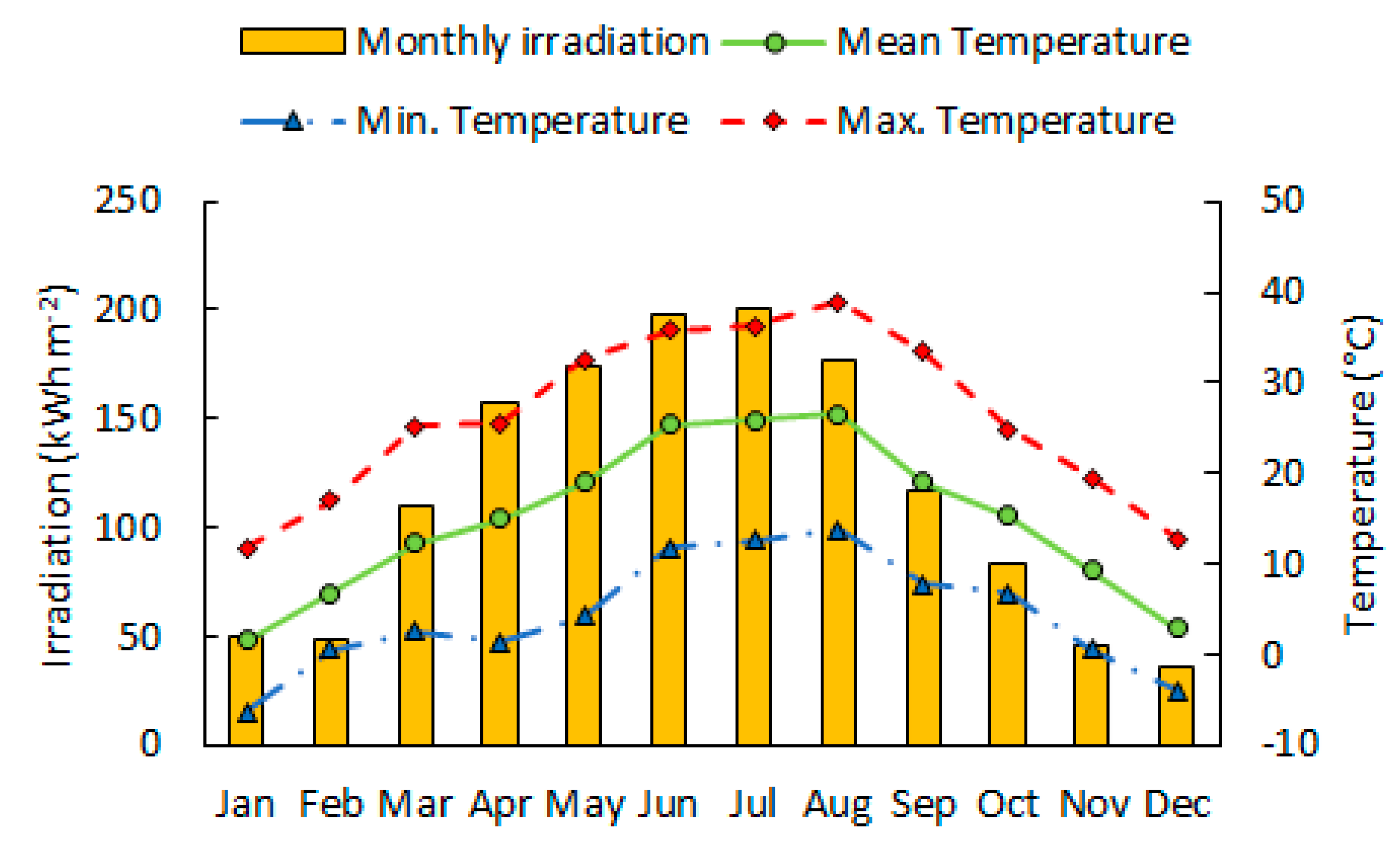
Monthly solar irradiation and outdoor temperatures for Milan [18] are shown in Figure 8. The weather conditions in Milan are characterized by an average daily irradiation on the horizontal plane equal to 3.8 kWh/m², mild cold temperatures during most of winter months and hot temperatures in the central summer months.

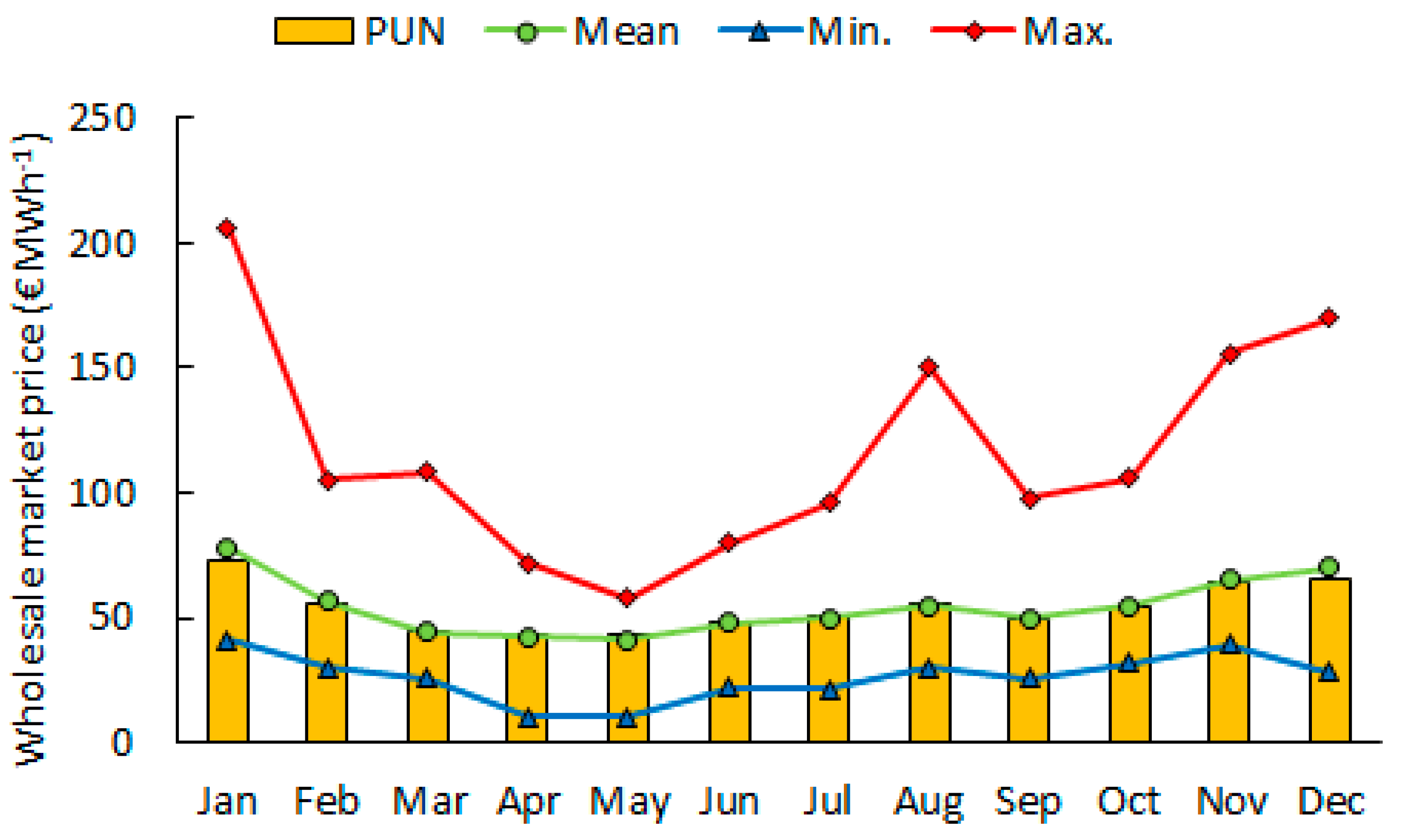
Energy prices on the electricity wholesale market [19] are shown in Figure 9, including the national average selling price and minimum, maximum, mean zonal prices for northern Italy. The maximum selling price deviates significantly from the average selling price, thus showing the potential economic margin deriving from PV electricity sold to the grid. The overall tariff related to the excess electricity sold to or purchased from the grid includes the contribution related to system charges and transmission and distribution costs, which is estimated equal to 55 €/MWh.

Concerning sewage water, its temperature is subject to seasonal variation due to the influence of weather. Based on direct measurements of treated water temperatures in Milano [12], a sinusoidal fluctuation from 13 °C in winter to 23 °C in summer can be assumed. This assumption is also supported by the measurements of the sewage temperature at the DHC in Budapest corrected by the shift between the average ambient temperatures of Budapest and Milano (2.5 K).

4.2. Heating and Cooling Loads

The total floor area of the commercial district is estimated at 12,000 m². Based on the building model input figures (see

Table A3. Building model input figures.

Parameter	Value	Unit
UA room air-outdoor air	26.8	kW/K
UA room air-envelope	120	kW/K
Thermal capacity of room air	87	MJ/K
Thermal capacity of envelope	1448	MJ/K
Occupation density	0.07	p/m2
Internal gain	15	W/m2
Ventilation	1	1/h
Infiltration	0.2	1/h
Solar radiation gain ratio	0.005	-
Comfort hours	8–21	hour
Heating/cooling active hours	4–21	hour
Cooling setpoint temperature	24	°C
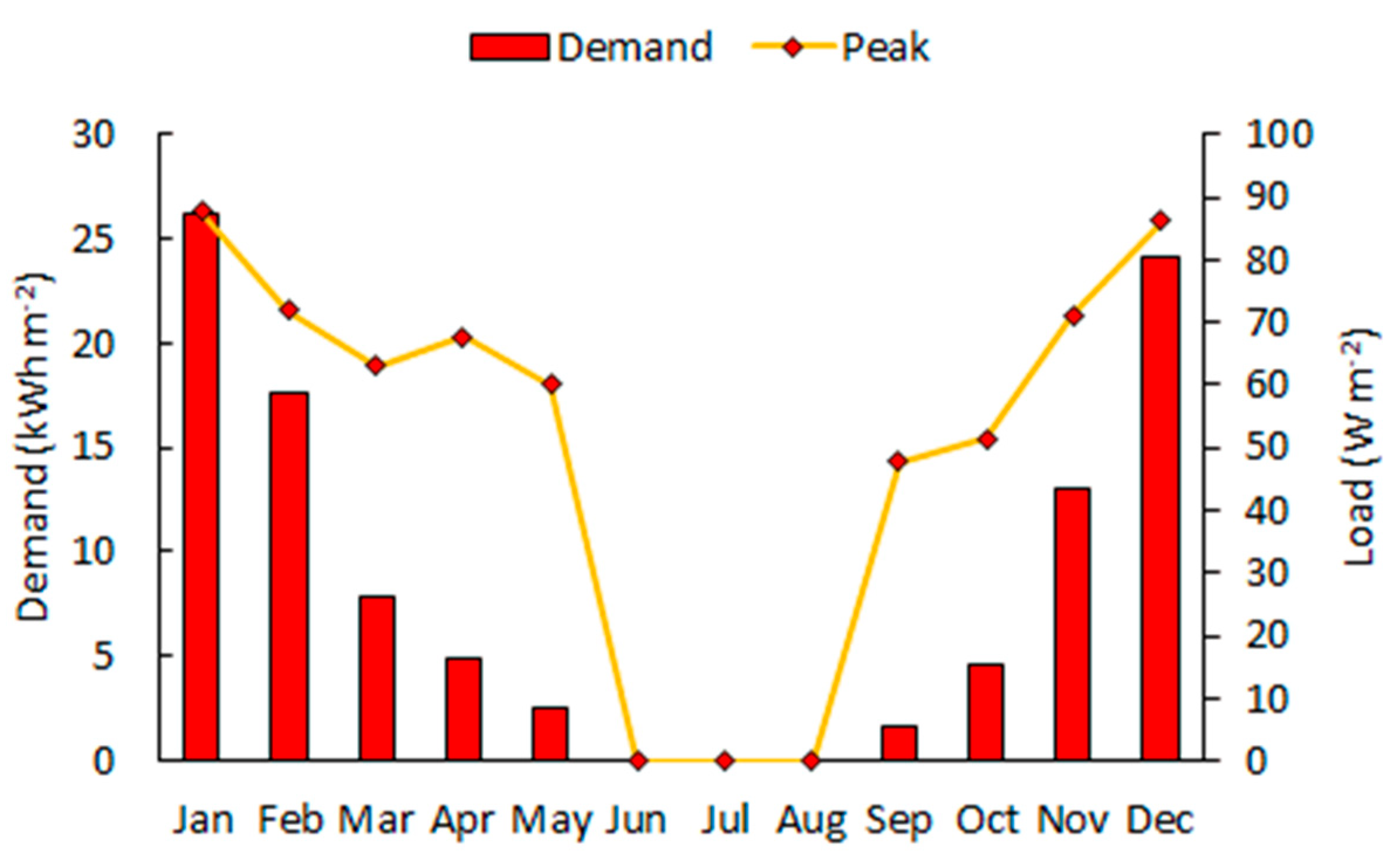
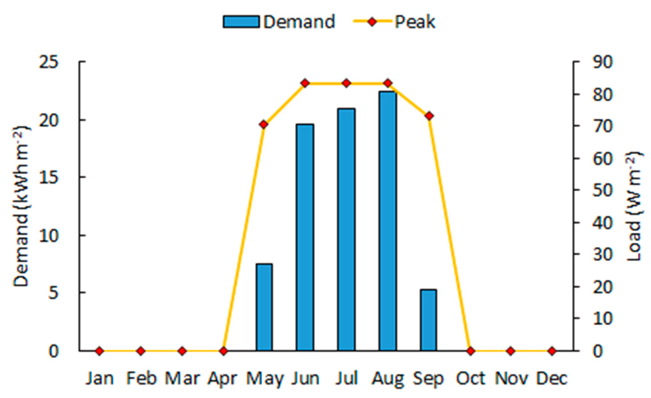
Heating setpoint temperature	22	°C

), heating and cooling hourly loads are calculated. The corresponding monthly values are shown in Figure 10 and Figure 11. The specific annual heating and cooling demands are 104 kWh/m² and 76 kWh/m², while the respective specific peak thermal loads are 87 W/m² and 83 W/m². These values are in line with the typical heating and cooling demands in the commercial sector in northern Italy. The overall heating and cooling annual demands are 1251 MWh and 912 MWh, and the peak loads are respectively 1050 kW_t and 1000 kW_t.

4.3. Plant Sizing

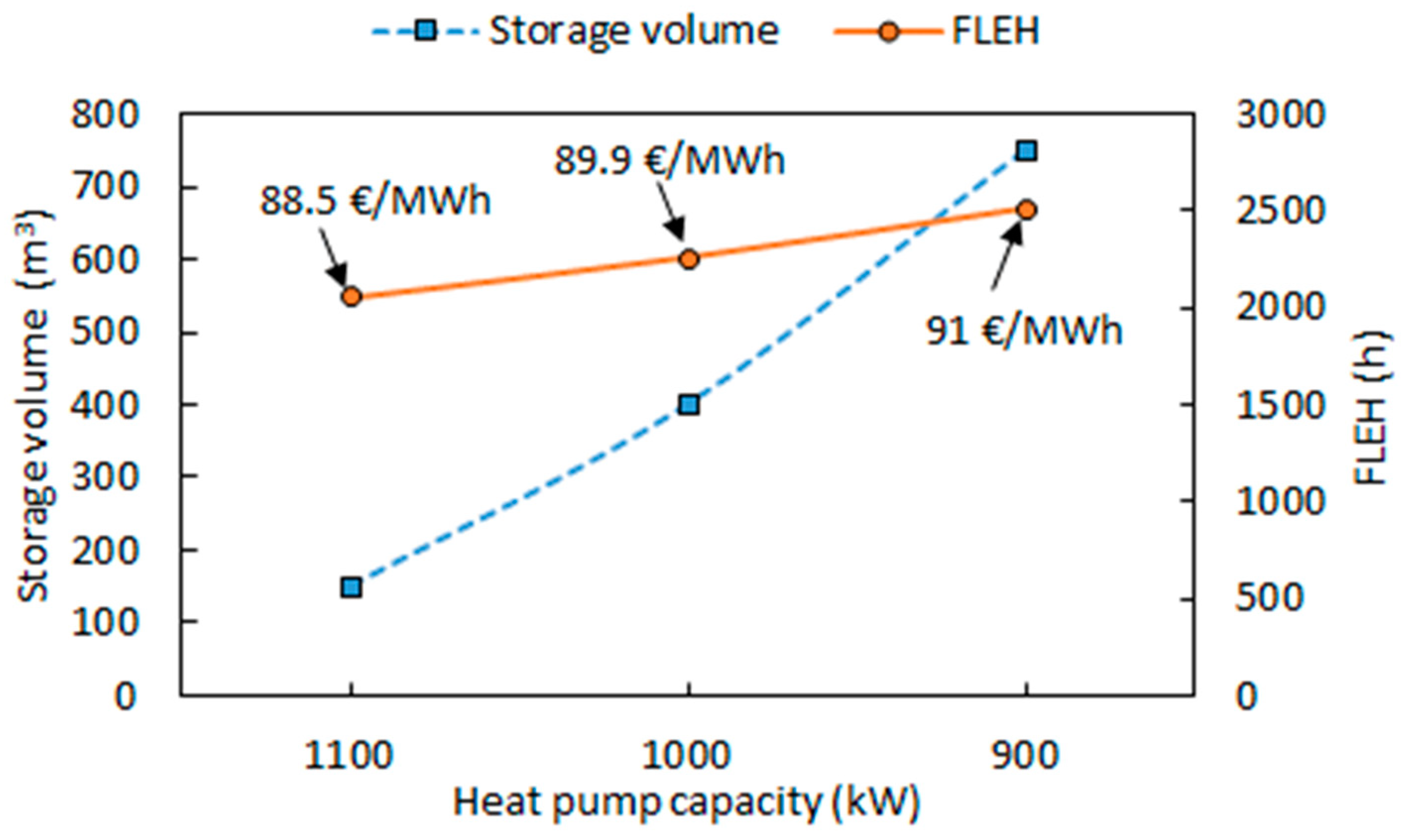
The DHC network supplies heat at 50 °C/40 °C and cool at 6 °C/13 °C. Based on the temperature differences and thermal loads, mass flow rates are derived. The preliminary sizing of the heat pump is performed according to the peak loads. As a first design value, a heat pump of $Q_{cond,nom}$ equal to 1100 kW is selected, and the heat duty of the sewage heat exchanger is determined as the maximum between evaporator heat duty in heating mode and condenser heat duty in cooling mode. Concerning the DHC network, the main design parameters are diameter and length of the pipeline. Pipeline diameter influences pressure drops and, ultimately, the parasitic energy consumption associated to the circulation pump of the DHC network. To limit this consumption, the design pressure drop at the circulation pump is fixed at 350 kPa, of which 50 kPa are associated to heat exchangers. Thus, the pipeline dimeter is selected to meet the net design pressure drop of 300 kPa at the required design volumetric flow rate. The DHC network design parameters are shown in

Table A4. Network design parameters for the reference scenario.

Parameter	Value	Unit
Peak heating load	1050	kW
Peak cooling load	1000	kW
Temperature difference, heating	10	K
Temperature difference, cooling	7	K
Volumetric flow rate	123	m3/h
Pipe length (one way)	1000	m
Water velocity	1.6	m/s
Backbone pipe internal diameter	160	mm
Backbone pipe external diameter	168	mm
Backbone insulation diameter	250	mm
Pressure drop (pipeline only)	300	kPa
Pressure drop (total, including HXs)	350	kPa

. The PV system area is an optimization parameter, since the remuneration of PV electricity sold the grid is penalized if the electricity in excess is larger than the electricity purchased. The optimum is achieved when total electricity exported to the grid is equal to the total electricity imported from grid on a yearly basis.

4.4. Cost Parameters

The estimated specific investment costs [20,21,22] are reported in

Table A5. Specific investment costs.

Item	Cost	Unit	Useful Life (y)	Annuity Factor (2.5%)
Heat storage	$13344V^{-0.595}$	€/m3	40	25.7
Substation	$35$	€/kW	20	16
Pipeline	$600$	€/m	40	25.7
Sewage screening and HX
A) machinery	$3784$	€ h/m3	15	12.7
B) construction	$5016$	€ h/m3	60	31.7
PV plant	$1400$	€/kWp	25	18.9
Screw chiller/heat pump	$150$	€/kWt	15	12.7

, along with the associated useful life and the resulting annuity factor, evaluated at an interest rate of 2.5%. Concerning maintenance, yearly maintenance costs are estimated equal to 1.5% of the investment cost of machineries. Lastly, the cost of each cleaning operation of the sewage heat exchanger is estimated at 500 €, assuming that the cleaning operation requires the work of one specialized technician for ten hours.

4.5. Reference System

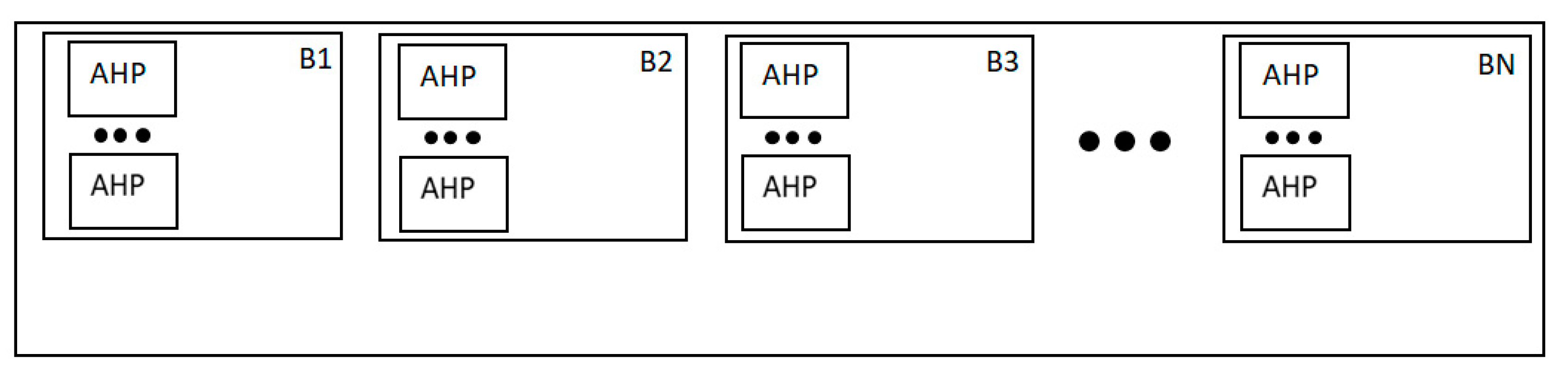
A reference system based on multiple, independent, reversible air-to-water heat pumps of small capacity is chosen as term for comparison with the system of interest (see Figure 12).

The individual heat pumps are assumed to deliver hot water at 50 °C for heating and chilled water at 7 °C for cooling. The specific investment cost of each unit is estimated at 340 €/kWh [23]. Hydraulics and electrical wiring costs are 30% of investment, and yearly maintenance is set to 1.5% of the investment. Since air-to-water units are installed outdoor, useful life is set to 10 years. At 2.5% interest rate, the corresponding annuity factor amounts to 8.97. In the reference scenario, the average cost of electricity for commercial users, equal to 150 €/MWh [24], is used. The overall installed capacity is determined by the peak heating load, since the heating capacity of air-to-water heat pumps is greatly reduced at the heating design condition. The installed heating capacity amounts to 1500 kW_t (at air temperature equal to 7 °C), which corresponds to 1150 kW_t at heating design condition (air temperature equal to −5 °C). The seasonal energy performance in heating and cooling is calculated dividing the heating and cooling hourly loads respectively by the instantaneous values of COP and EER, as provided by the manufacturer of a typical air-to-water heat pump [23]. The calculated seasonal COP and EER achieve respectively 2.41 and 3.27. The costs and the energy performance of the reference system are shown in

Table A6. CAPEX of the reference system.

Item	Cost	Useful Life (y)	Annuity (2.5%)
Air-source HPs (15 × 100 kW)	510,000	10	56,851
Hydraulics and electrical wiring	153,000	10	17,055
Total	663,000		73,906

,

Table A7. Energy performance of the reference system.

Figure	Value	Unit
Annual heating demand	1266	MWh
Annual cooling demand	912	MWh
Annual heating and cooling demand	2178	MWh
Heating demand system level (+5% losses)	1330	MWh
Cooling demand system level (+5% losses)	957	MWh
COP (heating, seasonal)	2.41	-
EER (cooling, seasonal)	3.27	-
Electricity demand	845	MWh

and

Table A8. OPEX of the reference system.

Cost Item	Value (€)
Maintenance (1.5%)	7650
Electricity purchase	126,708
Total	134,358

, while the calculation of its LCOHC, equal to 95.6 €/MWh, is reported in

Table A9. LCOHC of the reference system.

Cost Item	Value (€/MWh)
CAPEX	33.9
OPEX	61.7
total	95.6

.

5. Results

5.1. Parametric Analysis

The main goal of the parametric analysis is to perform an economical optimization of the DHC system by varying design parameters the mostly affect energy performance and life cycle cost. As a starting point, the preliminary size of the heat pump is set in order to satisfy both the heating and the cooling peak loads. Two other main parameters that greatly influence the overall investment cost are the volume of the storage ($V_s$, m³) and the nominal sewage flow rate of the SHX ($F_{shx}$, m³/h). As rule of thumbs, the volume of the storage is set to the volume of water crossing a section of the network in one hour, and the nominal sewage flow rate of the SHX is set equal to two-thirds the nominal flow rate of the heat pump (about 150 m³/h). Moreover, due to the progressive degradation of the SHX performance, periodical cleaning must be scheduled. The condition for cleaning is the maximum percentage reduction of flow passage area, set to a constant limiting value (50%). Lastly, it is decided to exclude the effect of PV during the optimization of heat pump capacity, storage volume and SHX. The base values of the main design parameters are reported in

Table 1. Initial configuration of the system.

Parameter	Value	Unit
Heat pump heating capacity	1100	kWt
Heat storage volume	150	m3
Sewage flow rate	100	m3/h
Reduction of flow passage	50	%

.

The first optimization step (see Figure 13) consists in decreasing heat pump capacity and simultaneously increasing storage volume. With a reduced capacity, the heat pump will work at full load for a larger number of hours, thus the FLEH is expected to increase. At the same time, a larger storage volume will be needed to cover the thermal peak loads. For each value of heat pump capacity, the minimum storage size is found iteratively until the yearly thermal demands are satisfied. It shall be noticed that the size of the sewage heat recovery system is maintained fixed at 100 m³/h.

It is observed that, although all the different configurations are cost competitive with respect to the reference system, the LCOHC increases with decreasing heat pump capacity because the benefit deriving from a smaller heat pump is offset by the cost of a larger storage.

The second step concerns the optimization of the size of the SHX (see Figure 14). Increasing its size while setting the same limiting flow passage area (in absolute terms) has an influence on the frequency of cleaning operations, since in a larger SHX that processes an equal amount of water the operating time needed to reach the critical flow passage area is prolonged. This lowers maintenance cost but also increases investment cost. In fact, cleaning maintenance decreases and LCOHC increases, showing that more frequent cleaning is always more economical than larger SHX size. However, it is also noticed that a larger SHX provides better energy performance with an increased system COP. This is because the heat pump is forced to operate in partial load whenever the sewage flow rate is reduced by effect of the SHX degradation. Therefore, as a best compromise between economic performance and risks associated to frequent cleaning, an optimal SHX size is selected at 110 m³/h.

Lastly, the contribution of PV is considered by progressively increasing the installed peak capacity until the minimum value for LCOHC is obtained. With 480 kWp of installed PV, the LCOHC decreased from 89.9 €/MWh to 79.1 €/MWh.

The final configuration of the system is reported in

Table 2. Final configuration of the system.

Parameter	Value	Unit
Heat pump heating capacity	1100	kWt
Heat storage volume	150	m3
Sewage flow rate	110	m3/h
Reduction of flow passage	55	%
PV capacity	480	kWp

.

5.2. Transient Operation

During the coldest winter days, the heat pump operates for several hours at its maximum heating capacity, as shown in Figure 15, where the profile of the heat supplied by the condenser (Q cnd) is shown, along with the heating load (Q use), for 21st January. The time shift between Q cnd and Q use is due to the thermal capacity of the storage and the pipeline. In the graph, the profile of different temperatures is also shown. T cnd,o and T use,i represent the hot water temperatures at condenser outlet and the user substation inlet, respectively. Their time shift and mean difference are an effect of thermal capacity and heat losses. T use,o, the return temperature at the user substation, is approximately 10 K lower than T use,i, even if the heating load profile varies between 400 kW and 1000 kW. This is the effect of the variable flow rate control strategy of the DHC network. In winter, the sewage water supplied to the SHX (T shx,i) is at about 13 °C. With the SHX clean, the sewage flow rate is high, as demonstrated by the limited temperature drop of about 7 K across the SHX between T shx,i and T shx,o. As consequence, the chilled water temperature leaving the heat pump evaporator T evp,o varies in the range from 2 °C to 6 °C, depending on the heat pump load. The difference between T shx,o and T evp,o is the pinch temperature difference, determined by the effectiveness of the SHX.

The behaviour of the system is investigated also when the SHX is fouled and the sewage water flow rate is reduced with respect to its nominal value (see Figure 16). The heat pump is forced to operate in partial load for the whole day to keep the chilled water in the heat pump evaporator sufficiently far from its freezing point. In this critical condition, storage thermal capacity is essential in order to cover the peak heating load.

Differently from the heating mode operation, during the hottest summer days the heat pump operates only for a few hours at its maximum cooling capacity, as shown in Figure 17, where the profile of the cool supplied by the evaportor (Q evp) is shown, along with the cooling load (Q use), for 27th July. This is due to the substantial difference in the way heating and cooling loads originate. In summer, the sewage is supplied to the SHX at a higher temperature of about 23 °C. With the SHX clean, the sewage flow rate is high, as demonstrated by the limited temperature rise of 10 K across the SHX between T shx,i and T shx,o. As consequence, the hot water temperature leaving the heat pump condenser T cnd,o varies in the range from 35 °C to 38 °C, depending on the load. The difference between T cnd,o and T shx,o is the pinch temperature difference, determined by the effectiveness of the SHX.

When the SHX is fouled, the sewage water flow rate is reduced with respect to its nominal value (see Figure 18) and the heat pump is forced to operate in partial load even when the cooling load is at its peak value to limit the temperature lift between evaporator and condenser. This strategy allows maintaining a good energy performance while limiting the temperature increase of the sewage.

5.3. Energy, Economic and Environmental Performance

The details about the calculation of LCOHC and the energy performance are reported in

Table 3. CAPEX of the DHC system.

Item	Amount (€)	Annuity (€/y)
PV system 480 kWp	672,840	35,628
Heat pump 1100 kwt	165,000	13,001
District H&C network
Pipeline 1 km	600,000	23,319
Storage 150 m3	101,532	3946
Substations 1000 kwt	35,000	2190
Sewage heat recovery 110 m3/h
A) machinery	416,240	32,798
B) construction & installation	551,760	17,416
Electrical connections	80,000	5007
Total	2,622,372	133,306

,

Table 4. Energy performance of the DHC system.

Figure	Value	Unit
Annual heating demand	1251	MWh
Annual cooling demand	912	MWh
Annual heating and cooling demand	2162	MWh
Heating demand including losses	1355	MWh
Cooling demand including losses	922	MWh
Heat pump COP (heating, seasonal)	3.74	-
Heat pump EER (cooling, seasonal)	4.03	-
System COP (heating, seasonal)	3.10	-
System EER (cooling, seasonal)	3.64	-
Electricity demand	634	MWh
PV electricity generation	637	MWh
Electricity exported to grid	360	MWh
Electricity imported from grid	356	MWh

,

Table 5. OPEX and annual benefit of the DHC system.

Cost Item	Value (€)
Maintenance	24,213
SHX cleaning	6500
Electricity purchase	43,169
Electricity sale	−32,264

and

Table 6. LCOHC of the DHC system.

Cost Item	Value (€/MWh)
CAPEX	61.7
OPEX	34.2
Benefits	−16.8
Total	79.1

. The CAPEX contribution to the total costs (i.e. CAPEX annuity plus OPEX) in the LCOHC is about 64%, with the SHX system representing the largest share (37%) of the total annuity cost of the system. Concerning OPEX, the estimated maintenance and cleaning costs are responsible for annual expenses of nearly 31 k€, about 42% of the total operating and maintenance costs. Despite the high investment costs, the overall economic performance is competitive, with a LCOHC of 79.1 €/MWh against 95.6 €/MWh for the reference system. The reasons for this are found in the superior energy performance of the DHC system, with system COP and EER of 3.10 and 3.64, higher than the respective values for the reference system (respectively 2.41 and 3.27), in the higher useful life of the DHC system, and in the largely positive contribution of the PV system that lowers LCOHC by 10.8 €/MWh. If PV is not installed, the superior energy performance of the DHC system alone can justify the investment with a LCOHC of 89.9 €/MWh. In this case, the electricity saving amounts to 211 MWh/y. Considering the carbon intensity of the Italian electric grid, which is estimated in 370 gCO₂/kWh and includes the share of renewable electricity [25], the associated avoided CO₂ emission amounts to 78 tCO₂/y.

6. Conclusions

According to the results of the present research, which are based on the detailed modelling of partial load operation and year-round simulations, a power to heat/cool system comprising sewage heat recovery, heat pump, storage, distribution network with substations, can be competitive with respect to individual, distributed, electricity driven heat pumps. With the addition of large-scale PV, the system can be even more competitive thanks to the remuneration of electricity sold to the grid and the large share of self-consumed PV electricity associated to the heating and cooling.

In the case of interest of this study, a commercial district located in northern Italy, the proposed DHC system can be an attractive solution. The overall LCOHC is 79.1 €/MWh against 95.6 €/MWh for the reference system considered (individual heat pumps). The reasons for this are found in: the superior energy performance of the DHC system, with system COP and EER of 3.10 and 3.64, higher than the respective values for the reference system (respectively 2.41 and 3.27); the longer useful life of the DHC system; and the largely positive contribution of the PV system that lowers LCOHC by 10.8 €/MWh. It shall be noticed that the superior energy performance of the DHC system can justify the investment even in absence of PV, with a LCOHC of 89.9 €/MWh. In this case, the electricity saving and the associated avoided CO₂ emission amount to 211 MWh/y and 78 tCO₂/y, respectively.

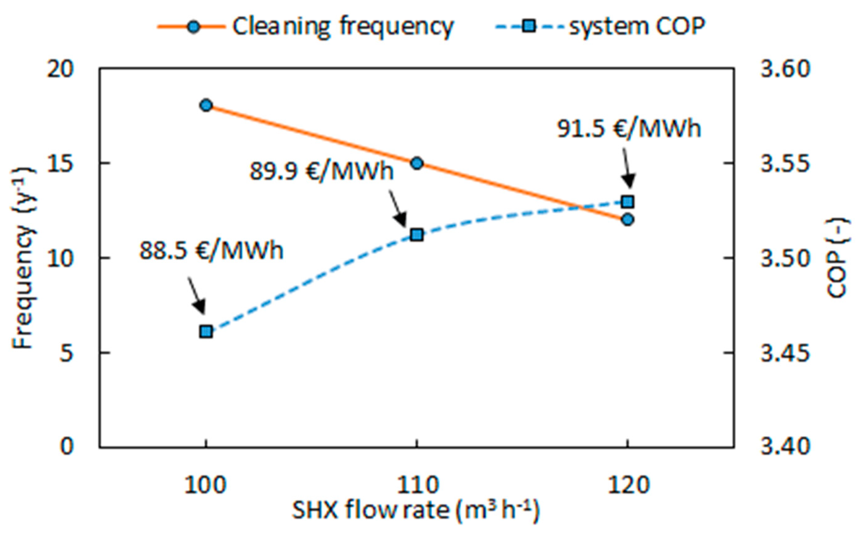
Although the results are specific for the location of interest and the regulation on distributed renewable electricity generation currently in place, they are promising. Commercial districts are interesting targets for DHC since heating and cooling intensity is expected to remain high. With new energy efficiency measures in buildings, cooling is expected to gain more importance than heating. Moreover, sewage is available with continuity of flow in large cities and represents an interesting thermal medium for heat source (in heating) and rejection (in cooling). The coexistence of heating and cooling loads in commercial buildings with sewage availability should be the driver for future researches on the potential of heating and cooling technologies complimented by sewage heat recovery. However, the analysis has also shown that the sewage heat recovery system is a rather expensive technology, and margin should exist to lower the associated investment costs and foster the replication of this solution. Moreover, frequent cleaning operations are needed. Cleaning frequency is tightly linked to sizing and an optimum size of sewage heat recovery system, heat pump and heat storage that allows maintaining cleaning at a manageable, cost-effective frequency must be pursued at design stage.