Abstract
Wind speed prediction is the key to wind power prediction, which is very important to guarantee the security and stability of the power system. Due to dramatic changes in wind speed, it needs high-frequency sampling to describe the wind. A large number of samples are generated and affect modeling time and accuracy. Therefore, two novel active learning methods with sample selection are proposed for short-term wind speed prediction. The main objective of active learning is to minimize the number of training samples and ensure the prediction accuracy. In order to verify the validity of the proposed methods, the results of support vector regression (SVR) and artificial neural network (ANN) models with different training sets are compared. The experimental data are from a wind farm in Jiangsu Province. The simulation results show that the two novel active learning methods can effectively select typical samples. While reducing the number of training samples, the prediction performance remains almost the same or slightly improved.
1. Introduction
Energy is the basic industry of the national economy, which plays an important role in guaranteeing the sustained development of the economy and the improvement of people’s lives. The shortage of fossil energy and its pollution has become the bottleneck of sustainable social and economic development. Sustainability transitions are necessary and long-term processes, which shift socio-technical systems to more sustainable modes of production and consumption. Better transitions can be achieved by adopting effective support policies of renewable energy and making concrete efforts to improve energy efficiency [1,2].
Wind energy is an important renewable energy source with the advantages of large reserves and wide distribution. Small-scale wind turbines are easy to transport and install. They are suitable for remote areas, mountainous areas, and islands [3,4]. As the cleanest source of renewable energy, wind power is rapidly becoming a potential and viable alternative energy source to burning fossil fuels. However, wind power generation has a high volatility and randomness. It may experience voltage fluctuation, even off-grid with large-scale wind power grid integration [5]. An accurate wind power prediction is necessary. Short-term wind speed prediction is the key to the safety and scheduling optimization of power systems [6].
In the prior literature, wind speed prediction methods are often divided into three categories based on different mechanisms: physical methods [7], time series methods [8], and machine learning methods [9,10]. The estimation of the wind speed can be considered as a nonlinear regression problem; therefore, machine learning methods are frequently adopted for short-term wind speed prediction with accurate results [11,12]. In [13], three forecasting techniques were compared: autoregressive moving average with generalized autoregressive conditional heteroskedasticity (ARMA-GARCH), artificial neural network (ANN), and support vector regression (SVR). The results showed that the SVR and ANN, with superior nonlinear fitting, obtained better forecasting accuracy. In [14], ANN was used to predict wind speed. The article used particle swarm optimization to select input parameters to achieve desired results. For machine learning methods, parameter optimization is a problem that needs to be studied. In [15], SVR combined with feature selection was used for wind speed prediction. It validated that SVR was suitable for short-term wind prediction, and that the performance of an SVR model could be improved by adding relevant input features. Machine learning is a data-driven decision or prediction through establishing a model from sample inputs. The forecasting performance also depends on the quantity and the quality of sample inputs used to train the regression and classification model.
Active learning, as a special case of a semi-supervised machine learning method, is used to deal with sample selection. The added new sample is to compensate for deficiencies in existing samples. It selectively queries some useful information to obtain the desired outputs at new data points. In statistics, it is also called optimal experimental design [16]. The active learning methods have often been successfully applied to classification problems [17,18]. In the work of Douak et al. [19], the active learning method was firstly used for wind speed prediction. The results showed that due to the ability to filter out the training samples, active learning could outperform full samples in some cases. However, the active learning method used in the article was based on the sample information and no model information was added. Based on this, two novel active learning algorithms coupled with model information for short-term wind speed forecasting models are proposed in this work. The motivation of this paper is to use the active learning method to predict short-term wind speed by optimizing the training sample sets, which can reduce the complexity of the model and ensure model accuracy. The main contents of the present work are to: 1) select the training samples by using two novel active learning methods, and 2) develop the prediction model for wind speed using ANN and SVR and compare the two active learning methods.
The remainder of this paper is organized as follows. Section 2 presents two novel active learning methods for forecasting wind speed. The experimental data and forecasting indexes are presented in Section 3. The results and performance analysis are discussed in Section 4. Finally, conclusions are drawn in Section 5.
2. Active Learning
The samples play an active role in the active learning process. The active learning method usually restricts the input area, then aims at sampling in the less redundant information input area. The samples that are most conducive to improving the performance of the training model are selected. The quality of training sets can be improved by active learning. The active learning mechanism is generally realized by the “Query” approach [20,21,22]. Firstly, select the initial training sample sets, then learn by some approach and add useful learning samples to the training sample sets. The training sample sets are obtained through continuous learning and optimization.
2.1. Euclidean Distance and Error (EDE-AL)
The first active learning approach (EDE-AL) is proposed by inserting samples that are distant from the current training samples, and removing samples by forecasting error. The Euclidean distances Edl = {Edl,t} (t = 1, 2,…, n) between each sample xl (l = n + 1, n + 2,…, n + m) of the learning subset Ui (i = 1, 2,…, k) and n different current training samples xt (t = 1, 2,…, n) are computed as follows:
After that, for each learning sample xl (l = n + 1, n + 2,…, n + m), the corresponding minimum distance value is considered as the addition criterion:
However, a single distance criterion cannot reflect the validity of samples well. The forecasting errors of the new additional samples are calculated and the samples with lower forecasting errors are removed from the training set.
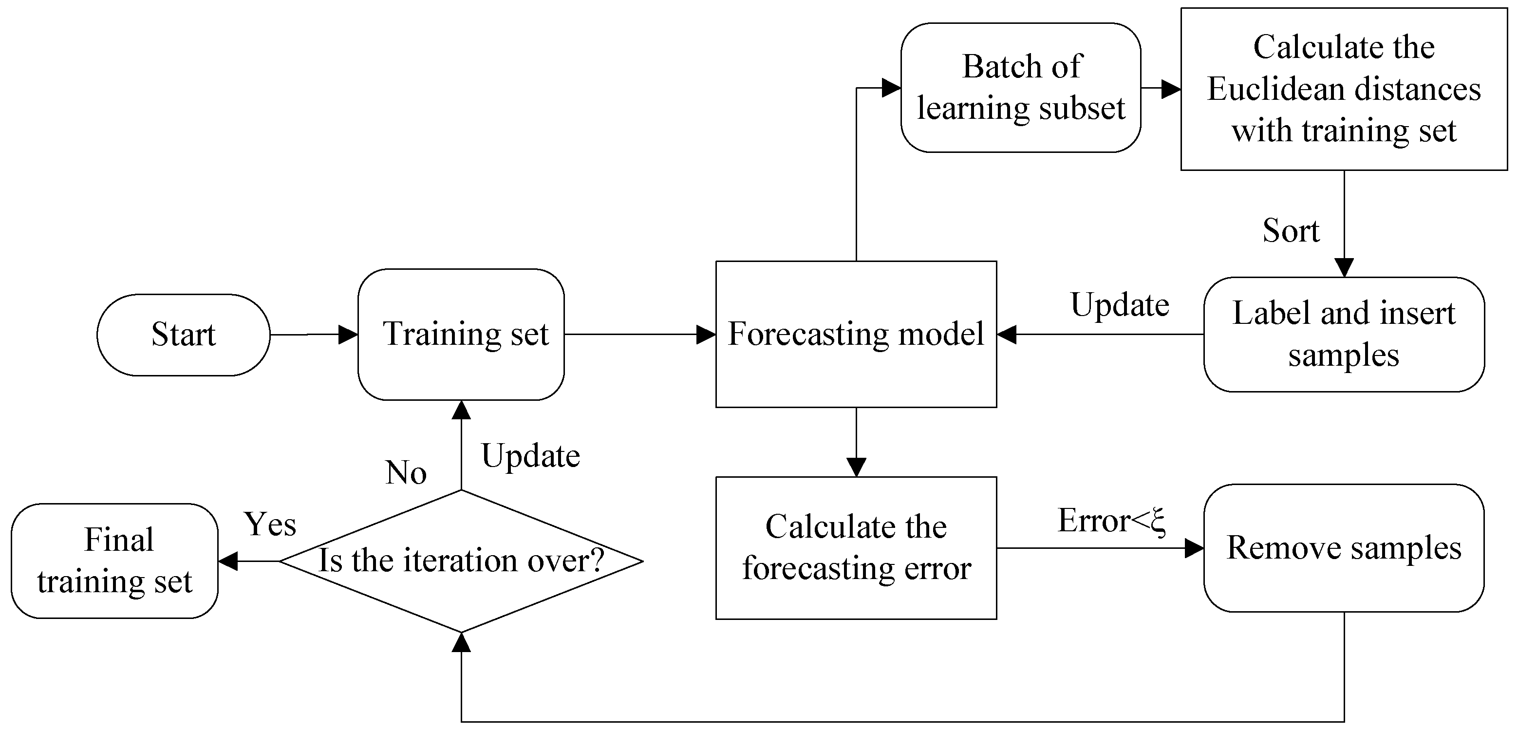
The strategy selects the samples with larger difference from the current training samples, and avoids choosing samples that are not useful for the model. The flow chart of the Euclidean distance combined with the forecasting error algorithm is shown in Figure 1 and summarized as follows:

Figure 1.
The flow chart of the active learning approach by Euclidean distance and error (EDE-AL).
- Step (1) Define the initial training samples xt (t = 1, 2,…, n) and the learning subset Ui (i = 1, 2,…, k);
- Step (2) Compute the Euclidean distances Edl = {Edl,t} (t = 1, 2,…, n) from the n different training samples xt (t = 1, 2,…, n) for each sample xl (l = n + 1, n + 2,…, n + m) of the learning subset;
- Step (3) Define the sample similarity as fED(l) = −min{Edl};
- Step (4) Label and insert the N most distant samples to the training set and update the forecasting model;
- Step (5) Calculate the forecasting errors of the new N training samples and remove samples with errors less than the threshold ξ;
- Step (6) Reestablish the model to predict the next learning subset until the iteration stops.
2.2. Support Vector Regression (SVR-AL)
In machine learning, the SVR algorithm is a supervised learning model used for regression analysis. The objective of SVR is to maximize the margin of separation and to minimize the misclassification error [23]. The SVR defines a loss function that ignores errors, which are situated within a certain distance of the true value. The function is often called ε-intensive loss function [24]. Figure 2 shows an example of a one-dimensional linear regression function with an ε-intensive band.
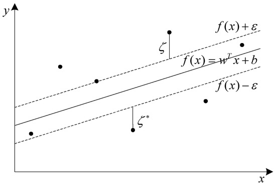
Figure 2.
One-dimensional linear regression with an epsilon intensive band.
So, the SVR optimization problem [25] is as follows:
where w is weight vector, C is a constant, and L is loss function
The above formula can be described by introducing slack variables , to measure the deviation of samples outside the ε-insensitive zone. Thus, SVR is formulated as minimization of the following function
Introducing Lagrange multipliers , , , and , the corresponding Lagrangian function can be written as
This in turn leads to the optimization problem
Introducing the kernel function, the above formula is written as
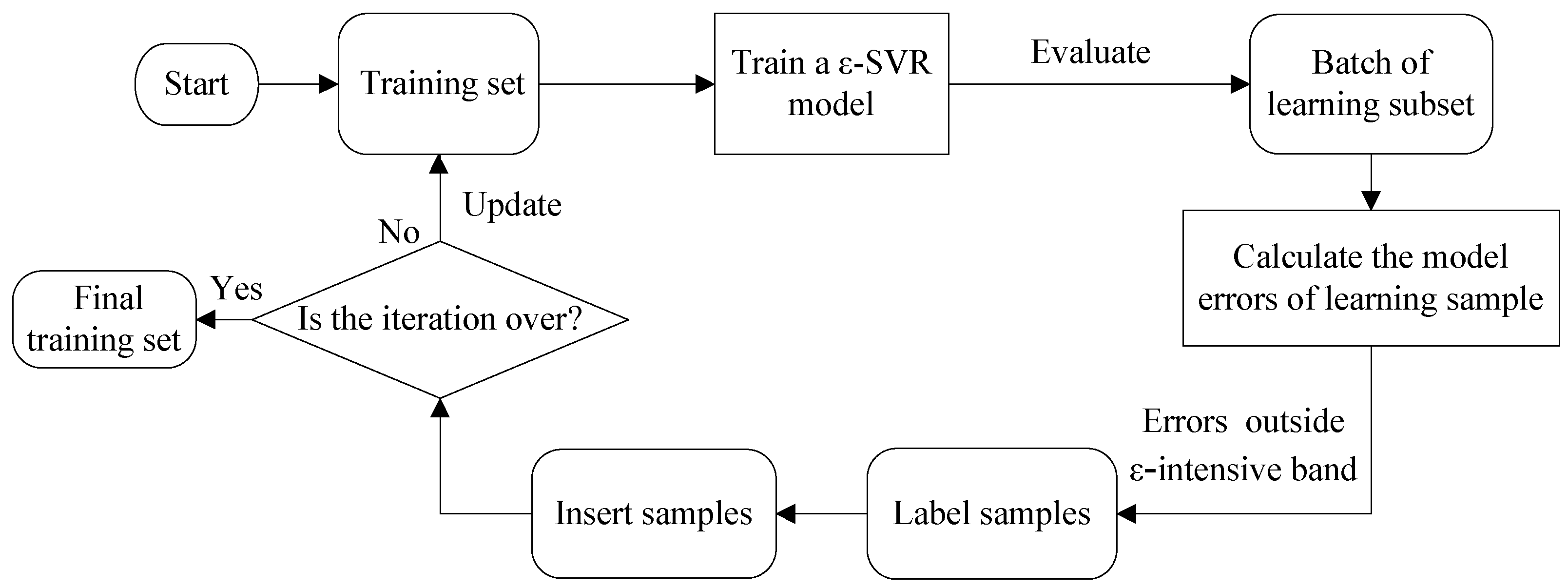
Uncertainty sampling is the main strategy of active learning methods. Geometrically, the sample errors outside ε-intensive bands have great uncertainty and are important to the final design of the model. The proposed strategy selects the samples with uncertainty information. The flow chart of the SVR-AL algorithm is shown in Figure 3 and summarized as follows:
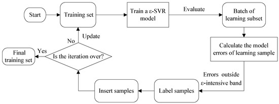
Figure 3.
The flow chart of the active learning approach by support vector regression (SVR-AL).
- Step (1) Define the initial training samples xt (t = 1, 2,…, n) and the learning subset Ui (i = 1, 2,…, k);
- Step (2) Establish an ε-SVR model by using training samples, and calculate the model error of each sample xl (l = n + 1, n + 2,…, n + m) of the learning subset;
- Step (3) Label and insert the samples with model errors outside the ε-intensive band into the training set;
- Step (4) Update the training set and reestablish the ε-SVR model to predict the next learning subset until the iteration stops.
3. Materials and Experiment
3.1. Wind Speed Data Sets
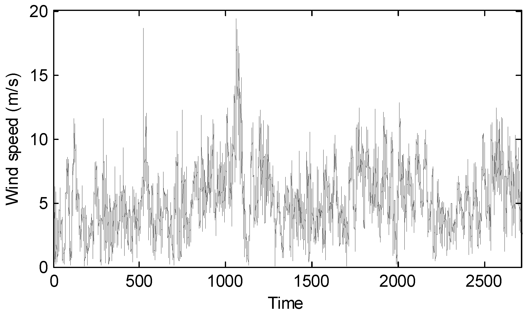
The wind speed data were collected from a wind farm in Jiangsu Province in China. The acquisition equipment is a low-wind-speed wind turbine FD-77 with 1.5 MW rated power. The turbine is composed of three blades with a diameter of 77 m and a sweep area of 4657 m2. The collected wind information included real-time wind direction and speed, 5-min average wind speed, and standard deviation.
The 30-min average wind speed was calculated and used in the experiment from 1 June 2011 to 30 July 2011. There were 2729 groups of data. The first 2000 data were used as a training set and the remaining 729 data were for testing. The typical samples were selected from the training set. Therefore, the training set was divided into an initial training set and learning subsets. The first 100 data were used for the initial training set and then each of 100 samples was a learning subset. The final training set was used to train the models for short-term wind speed prediction, and the testing set was used to compare the performance of the two active learning strategies. Figure 4 displays the wind speed time series. Table 1 shows the descriptive statistics of different wind speed datasets.
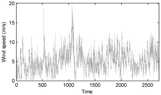
Figure 4.
The wind speed data in Jiangsu wind farm.

Table 1.
Descriptive statistics of wind speed datasets (m/s).
3.2. Model Selection
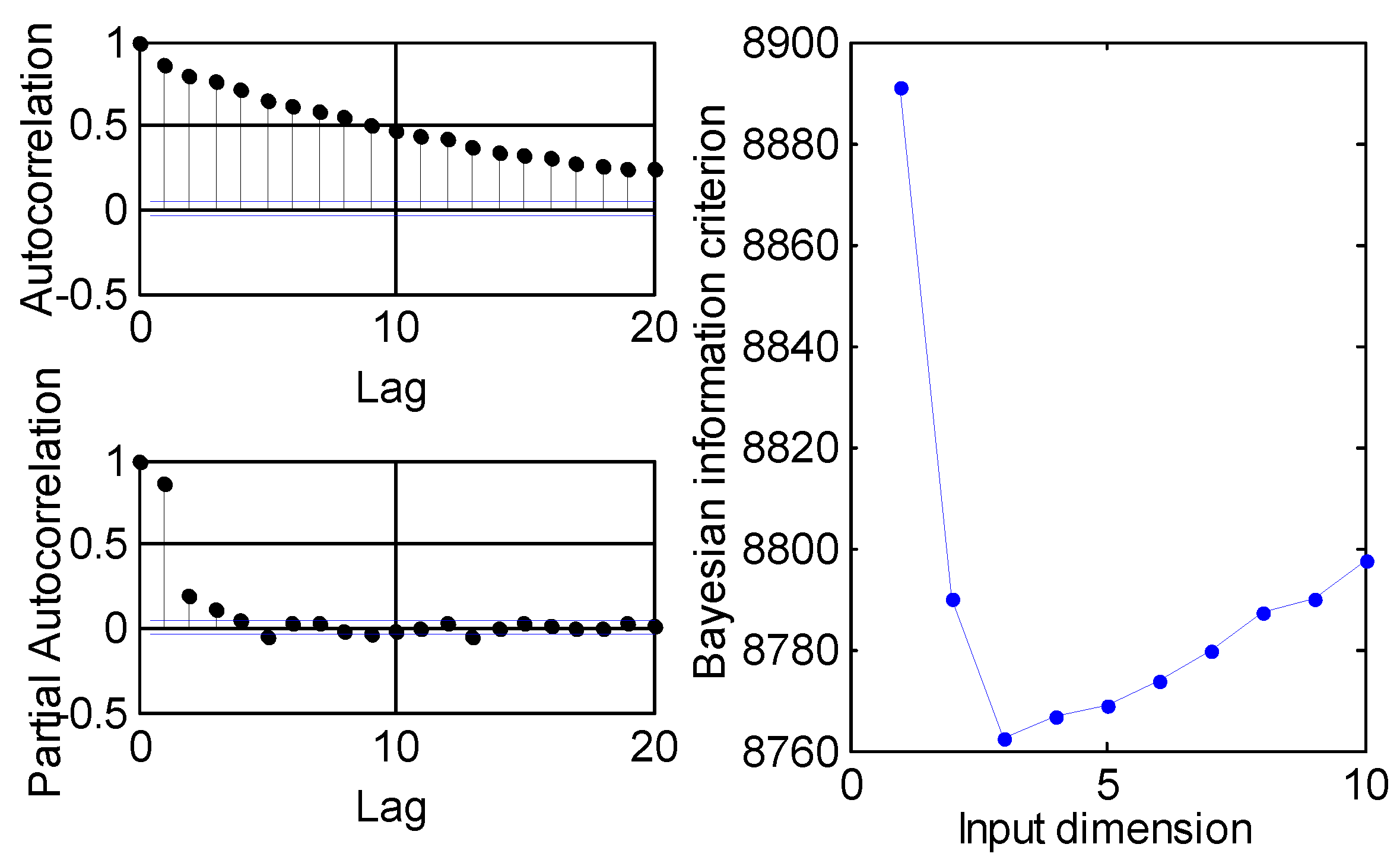
Model selection selects a certain structural statistical model from a set of given data. If the input dimension is too small, the input information is not enough and the prediction accuracy will be reduced. If the input information is redundant, the complex prediction model will also reduce the prediction accuracy [26]. The criterion function method is to determine the degree of approximation of the original data based on the residual value. Bayesian information criterion (BIC) is a criterion for model selection and the model with the lowest BIC is preferred. In this paper, the BIC function method was used to determine the model input dimension. The autocorrelation function (ACF) and partial autocorrelation function (PACF) were also used to identify the input dimension. The PACF is zero at lag p + 1 and greater, so the appropriate lag is the one beyond which the partial autocorrelations are all zero. According to the result of PACF and BIC criterion (Figure 5), the input dimension of the model was 3.
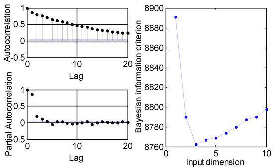
Figure 5.
The result of input dimension selection.
3.3. Prediction Models
The ANN and SVR were used to develop the prediction models for short-term wind speed. The multilayer perceptron (MLP) is one of the most popular ANN algorithms [27]. In this study, MLP was used with an input layer, a hidden layer, and an output layer. There were 3 input nodes, 6 hidden-layer nodes, and 1 output node. The transfer function on the hidden layer was a sigmoid function and the training algorithm was Levenberg-Marquardt.
The SVR is a popular non-linear modeling tool. The SVR maps the input data into a high dimensional feature space via a kernel [28]. In this study, a radial basis kernel was used for SVR, and the gradient optimization method was used to determine two important parameters: the penalty coefficient and the width of the RBF kernel function.
The models are evaluated synthetically using the following evaluation criteria. The main variables in this paper are shown in the Table 2.
Table 2.
The description of the main variables.
(1) root mean square error (RMSE)
(2) mean absolute error (MAE)
(3) mean absolute percentage error (MAPE)
where and are the measured and predicted wind speed, respectively, at time t, and M is the number of test data.
4. Results and Discussion
In order to better verify the effectiveness of the two proposed active learning methods, the random selection of a similar number of samples was used for comparison. The model was used for 1-step ahead (30 min) and 4-step ahead (2 h) wind speed prediction. The prediction results combining different models and different training sets are shown in Table 3 and Table 4. From Table 3 and Table 4, it can be seen that the number of training samples were both reduced by half by using two proposed active learning methods, and the performance was similar to the all training samples model. Comparing the results of different models, the persistence model had the worst performance and the SVR model was more suitable for wind speed prediction than the ANN model.
Table 3.
1-step ahead (30 min) prediction of short-term wind speed with different sample sets. ANN is artificial neural network. SVR is support vector regression.
Table 4.
4-step ahead (2 h) prediction of short-term wind speed with different sample sets.
Table 4 shows the results of the 1-step ahead (30 min) prediction; it can be seen that the RMSE with all training samples was the best. This means that the model could be trained more adequately with all training samples. However, the ANN model with the typical samples selected by EDE-AL could obtain a similar RMSE and a relatively better MAPE and MAE. At the same time, the MAE and MAPE by the SVR model with SVR-AL sample sets were lowest. The performances of the two active learning methods were better than that of the similar number of random training samples. Compared to the performance of all training sample set, the performances of two active learning methods were similar or slightly worse. The numbers of training samples were reduced by about 60%. Two active learning methods combined with different models had different performances. In conclusion, these two methods significantly reduced the training samples and ensured model accuracy.
Table 4 shows the results of 4-step (2 h) ahead prediction. The RMSE, MAE, and MAPE were poorer than 1-step ahead prediction. Compared to the all training samples, the numbers of training samples by EDE-AL and SVR-AL were reduced by 34 percent. Meanwhile, the two active learning methods outperformed the random method. The performance discrepancy between the two active learning methods was not obvious.
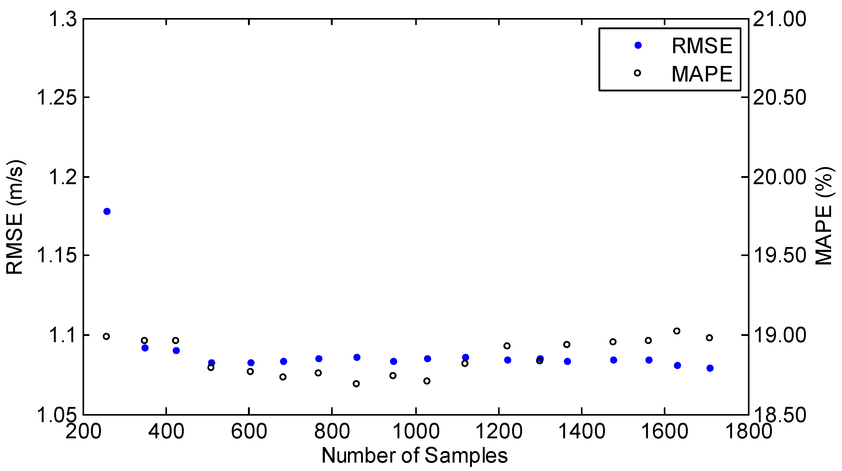
Figure 6 and Figure 7 show the 1-step ahead prediction results by two active learning methods combined with SVR models for short-term wind speed.
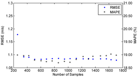
Figure 6.
1-step ahead prediction results of the support vector regression (SVR) model by EDE-AL with ξ = 0.54 and different N values.
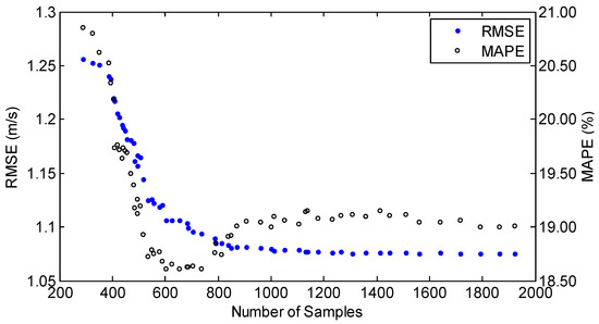
Figure 7.
1-step ahead prediction results of SVR model by SVR-AL with different ε values.
For EDE-AL, two parameters needed to be determined. The larger the N, the more samples were labeled and added. The larger the ξ, the more samples were removed. When the forecasting errors of samples were less than half of the RMSE of all training sample sets, we argued that the samples were useless for the model. Therefore, ξ was chosen to be half of the RMSE of all training sample sets and N was variable. From Figure 6, it can be seen that the changes of RMSE and MAPE were moderate. When the number of training samples was 847, the MAPE was minimal and RMSE was relatively large. Therefore, the point at 680 was selected with relatively small values of RMSE and MAPE at the same time.
For SVR-AL, the number of additional samples gradually increases as ε becomes smaller. From Figure 7, it can be seen that the RMSE gradually decreased as the number of samples increased. However, the MAPE between 600–800 was significantly less than that of the all training sample set. The samples outside the ε-insensitive zone generally fluctuated greatly. Due to the addition of these samples, the marginal samples had better predictions. More intermediate samples were added as ε became smaller. Therefore, the MAPE decreased first and then increased.
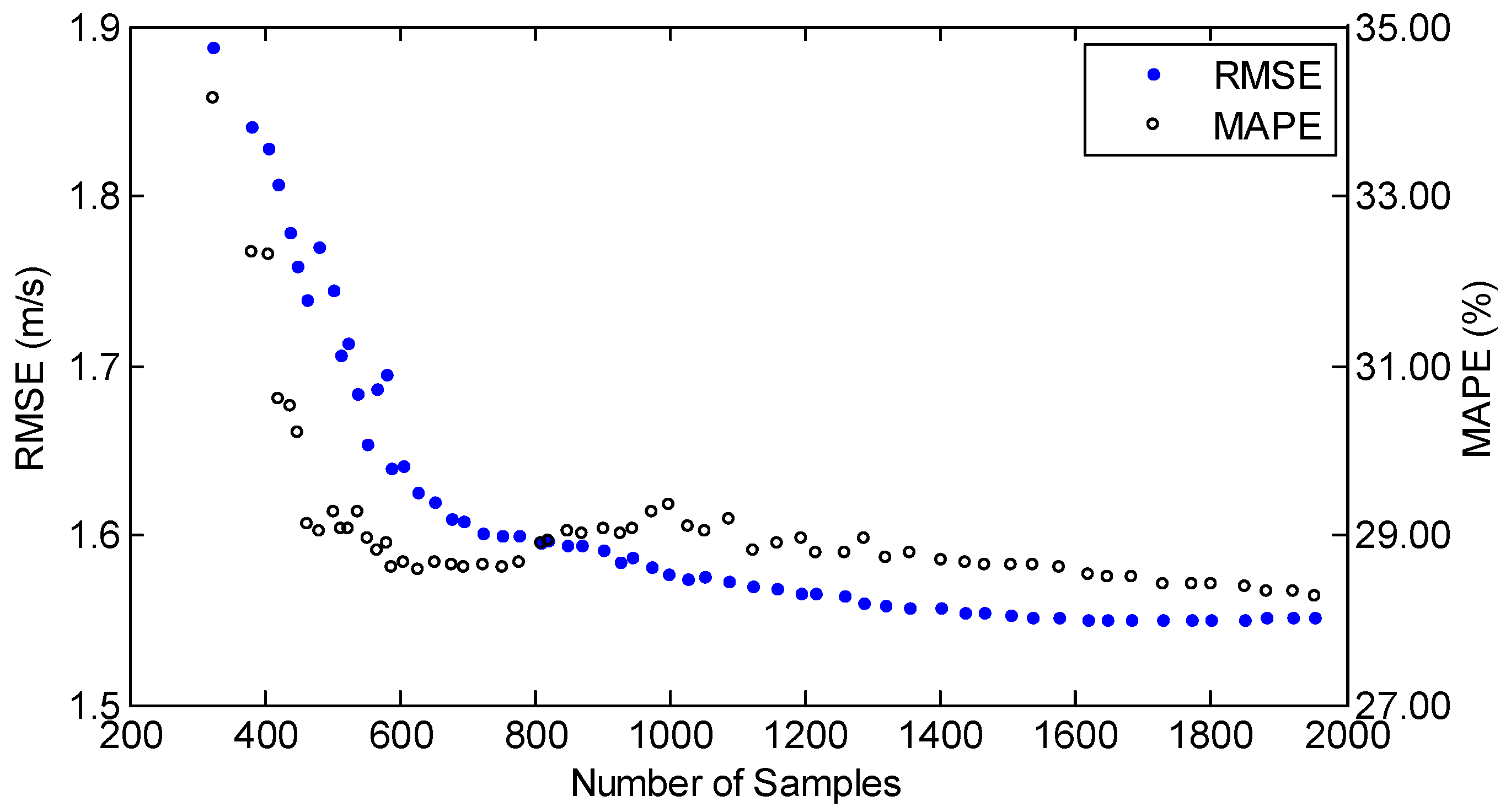
Figure 8 and Figure 9 show the 4-step ahead prediction results by two active learning methods combined with SVR models for short-term wind speed. Compared with 1-step ahead prediction results, the performance of 4-step ahead prediction was poor and the trends of RMSE and MAPE were consistent.
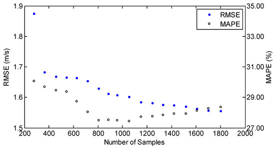
Figure 8.
4-step ahead prediction results of the SVR model by EDE-AL with ξ = 0.79 and different N values.
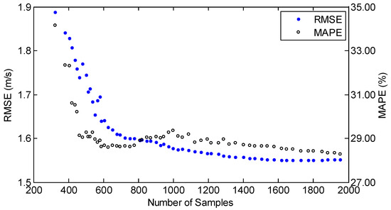
Figure 9.
4-step ahead prediction results of the SVR model by SVR-AL with different ε values.
5. Conclusions
Active learning was used to select samples for short-term wind speed prediction in this study. Starting from the initial training set, the proposed method selected typical samples from a large number of samples. Two novel active learning methods using model information to label and add samples were proposed in this study. The ANN and SVR models combined with two novel active learning methods were investigated for 1-step (30 min) and 4-step (2 h) ahead wind speed prediction. The results showed that the EDE-AL and SVR-AL had better performance than the random approach. Compared with all the training samples, the selected samples by the proposed methods were significantly reduced, while ensuring model accuracy.
Author Contributions
J.Y. and X.Z. contributed equally to this work. H.W. and K.Z. proposed the concept of this research and provided overall guidance. J.Y. and X.Z. worked in the design of two active learning methods and the simulations.
Funding
This work was supported by the National Natural Science Foundation of China (Grant No. 61773118 and Grant No. 61703100).
Conflicts of Interest
The authors declare no conflicts of interest.
Abbreviations
Abbreviations in this manuscript are summed up as follows:
| ANN | Artificial neural network |
| SVR | Support vector regression |
| MLP | Multilayer perceptron |
| EDE-AL | Active learning approach by Euclidean distance and error |
| SVR-AL | Active learning approach by support vector regression |
| BIC | Bayesian information criterion |
| ACF | Autocorrelation function |
| PACF | Partial autocorrelation function |
| RMSE | Root mean square error |
| MAE | Mean absolute error |
| MAPE | Mean absolute percentage error |
References
- Ponta, L.; Raberto, M.; Teglio, A.; Cincotti, S. An agent-based stock-flow consistent model of the sustainable transition in the energy sector. Ecol. Econ. 2018, 145, 274–300. [Google Scholar] [CrossRef]
- De Filippo, A.; Lombardi, M.; Milano, M. User-Aware electricity price optimization for the competitive market. Energies 2017, 10, 1378. [Google Scholar] [CrossRef]
- Jung, J.; Broadwater, R.P. Current status and future advances for wind speed and power forecasting. Renew. Sustain. Energy Rev. 2014, 31, 762–777. [Google Scholar] [CrossRef]
- Zhou, J.; Sun, N.; Jia, B.; Peng, T. A novel decomposition-optimization model for short-term wind speed forecasting. Energies 2018, 11, 1752. [Google Scholar] [CrossRef]
- Li, G.; Shi, J.; Zhou, J. Bayesian adaptive combination of short-term wind speed forecasts from neural network models. Renew. Energy 2011, 36, 352–359. [Google Scholar] [CrossRef]
- De Giorgi, M.G.; Campilongo, S.; Ficarella, A.; Congedo, P.M. Comparison between wind power prediction models based on wavelet decomposition with least-squares support vector machine (LS-SVM) and artificial neural network (ANN). Energies 2014, 7, 5251–5272. [Google Scholar] [CrossRef]
- Howard, T.; Clark, P. Correction and downscaling of NWP wind speed forecasts. Meteorol. Appl. 2010, 14, 105–116. [Google Scholar] [CrossRef]
- Carta, J.A.; Ramírez, P.; Velázquez, S. A review of wind speed probability distributions used in wind energy analysis: Case studies in the Canary Islands. Renew. Sustain. Energy Rev. 2009, 13, 933–955. [Google Scholar] [CrossRef]
- Liu, D.; Niu, D.; Wang, H.; Fan, L. Short-term wind speed forecasting using wavelet transform and support vector machines optimized by genetic algorithm. Renew. Energy 2014, 62, 592–597. [Google Scholar] [CrossRef]
- Liu, H.; Tian, H.; Li, Y.; Zhang, L. Comparison of four Adaboost algorithm based artificial neural networks in wind speed predictions. Energy Convers. Manag. 2015, 92, 67–81. [Google Scholar] [CrossRef]
- Ak, R.; Fink, O.; Zio, E. Two machine learning approaches for short-Term wind speed time-series prediction. IEEE Trans. Neural Netw. Learn. Syst. 2016, 27, 1734–1747. [Google Scholar] [CrossRef]
- Han, Q.; Wu, H.; Hu, T.; Chu, F. Short-term wind speed forecasting based on signal decomposing algorithm and hybrid linear/nonlinear models. Energies 2018, 11, 2796. [Google Scholar] [CrossRef]
- Cincotti, S.; Gallo, G.; Ponta, L.; Raberto, M. Modeling and forecasting of electricity spot-prices: Computational intelligence vs classical econometrics. AI Commun. 2014, 27, 301–314. [Google Scholar]
- Ren, C.; An, N.; Wang, J.; Li, L.; Hu, B.; Shang, D. Optimal parameters selection for BP neural network based on particle swarm optimization: A case study of wind speed forecasting. Knowl.-Based Syst. 2014, 56, 226–239. [Google Scholar] [CrossRef]
- Kong, X.; Liu, X.; Shi, R.; Lee, K.Y. Wind speed prediction using reduced support vector machines with feature selection. Neurocomputing 2015, 169, 449–456. [Google Scholar] [CrossRef]
- Cohn, D.A.; Ghahramani, Z.; Jordan, M.I. Active Learning with Statistical Models. J. Artif. Intell. Res. 1996, 4, 705–712. [Google Scholar] [CrossRef]
- Cohn, D.; Atlas, L.; Ladner, R. Improving Generalization with Active Learning. Mach. Learn. 1994, 15, 201–221. [Google Scholar] [CrossRef]
- Tuia, D.; Ratle, F.; Pacifici, F.; Kanevski, M.; Emery, W. Active learning methods for remote sensing image classification. IEEE Trans. Geosci. Remote. 2009, 47, 2218–2232. [Google Scholar] [CrossRef]
- Douak, F.; Melgani, F.; Benoudjit, N. Kernel ridge regression with active learning for wind speed prediction. Appl. Energy 2013, 103, 328–340. [Google Scholar]
- Zliobaite, I.; Bifet, A.; Pfahringer, B.; Holmes, G. Active learning with drifting streaming data. IEEE Trans. Neural Netw. Learn. Syst. 2014, 25, 27–39. [Google Scholar] [CrossRef]
- Huang, S.; Jin, R.; Zhou, Z. Active learning by querying informative and representative examples. IEEE Trans. Pattern Anal. 2014, 36, 1936–1949. [Google Scholar] [CrossRef] [PubMed]
- Gal, Y.; Islam, R.; Ghahramani, Z. Deep Bayesian Active Learning with Image Data. Available online: https://arxiv.org/abs/1703.02910 (accessed on 8 March 2017).
- Chen, Y.; Xu, P.; Chu, Y.; Li, W.; Wu, Y.; Ni, L.; Bao, Y.; Wang, K. Short-term electrical load forecasting using the Support Vector Regression (SVR) model to calculate the demand response baseline for office buildings. Appl. Energy 2017, 195, 659–670. [Google Scholar] [CrossRef]
- Zhou, X.; Jiang, T. An effective way to integrate ε-support vector regression with gradients. Expert Syst. Appl. 2018, 99, 126–140. [Google Scholar] [CrossRef]
- Ma, J.; Theiler, J.; Perkins, S. Accurate on-line support vector regression. Neural Comput. 2003, 15, 2683–2703. [Google Scholar] [CrossRef] [PubMed]
- Vrieze, S.I. Model selection and psychological theory: A discussion of the differences between the Akaike information criterion (AIC) and the Bayesian information criterion (BIC). Psychol. Methods 2012, 17, 228–243. [Google Scholar] [CrossRef] [PubMed]
- Azimi, R.; Ghofrani, M.; Ghayekhloo, M. A hybrid wind power forecasting model based on data mining and wavelets analysis. Energy Convers. Manag. 2016, 127, 208–225. [Google Scholar] [CrossRef]
- Santamaria-Bonfil, G.; Reyes-Ballesteros, A.; Gershenson, C. Wind speed forecasting for wind farms: A method based on support vector regression. Renew. Energy 2016, 85, 790–809. [Google Scholar] [CrossRef]


© 2019 by the authors. Licensee MDPI, Basel, Switzerland. This article is an open access article distributed under the terms and conditions of the Creative Commons Attribution (CC BY) license (http://creativecommons.org/licenses/by/4.0/).