1. Introduction
The current worldwide energy transition from conventional to renewable energy sources already proves and even more forecasts the expansion of photovoltaic systems to new and diverse locations. On a global scale, we are rapidly approaching the so-called “Terawatt-scale Photovoltaics” era, which indicates the surpass of 1 TW of installed capacity of photovoltaic (PV) systems and highlights an important milestone for the PV industry [
1]. This milestone is also boosted by the decrease in prices of the PV technologies, which are already the cheapest source of electricity in many countries of Europe [
2].
However, this diversification is presenting some constraints in terms of financial and technical risks, due to the unclear response of PV modules and materials under different climate conditions. The financial risks are related to the estimation of the long-term energy yield, mainly due to degradation rate calculations and solar resource variability, as represented by calculations of Levelized-Cost-Of-Electricity (LCOE) for PV systems. The technical risks are related to the failure modes prone to occur for different Bill-of-Materials (BOM) and Balance-of-System (BOS) under different climatic stresses which will vary from location to location. For example, while in deserts the risk of sand-storms is high, in highlands wind gusts and snow loads can damage the PV installations. Important findings and calculation methods about the climatic triggers of degradation modes under different climate zones have been presented in [
3,
4,
5,
6,
7,
8,
9,
10,
11]. Irradiation, temperature, and humidity have been identified as the main degradation precursors, leading to different degradation mechanisms depending on the stress level in each climate zone. In qualitative terms, some generalizations can be made by climate: in tropical climates, the combination of high humidity and high temperature is stated as being the harshest for PV reliability, where the PV modules are prone to delamination, corrosion or Potential-Induced-Degradation (PID). Desert and steppe climates stimulate degradation modes, such as encapsulant discoloration, backsheet chalking or delamination. Temperate, cold and polar climates typically present low degradation due to the low climatic stress, but modules are prone to fast power drops due to hail, storms or snow loads inducing cell cracks, glass cracks and interconnect breakage. In quantitative terms, Jordan et al. have been the pioneers in the degradation rate assessment under different climate conditions [
4], but the complexity of the issue does not yet allow the conclusion of a generalized estimation model per climate zone. The synergy of climate stressors makes the estimation and prediction of the degradation rates (i.e., expressed as a reduction of the power per year, %/a) not trivial, given that not only different module types react differently regarding the climate but also that material interactions will behave differently [
6].
Studies at a global scale present the mapping of PV performance indicators (e.g., performance ratio and energy yield) using different Geographic Information Systems (GIS) datasets and approaches [
12,
13,
14]. Regarding the long-term operation of PV systems, usually this issue is simplified by considering a typical value (i.e., 0.5%/a for crystalline PV modules), also stated on manufacturer performance warranties. However, it is known that the impact of climate on material properties and energy production will vary over time and location. Interesting approaches to calculate the degradation rates have been proposed in references [
10,
15]. Both models consider as main climate degradation factors the average temperatures, temperature changes, humidity, and ultraviolet (UV) irradiation, which is in line with indoor testing and standards for PV reliability. However, those models have not been applied at global scale and a PV degradation mapping has not been published so far.
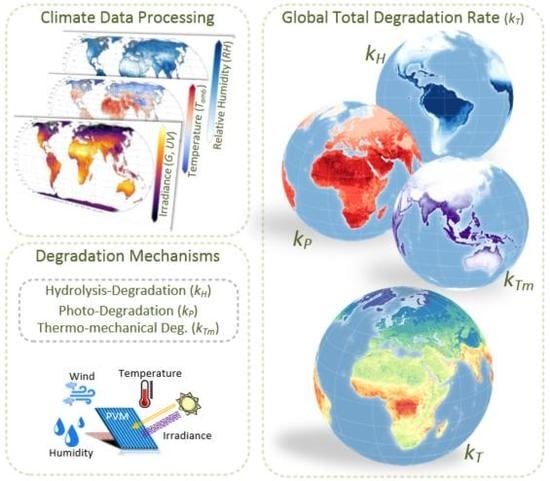
In this paper, the ERA5 climate reanalysis dataset [
16] is processed to extract and further to model the essential climate variables for the study of PV degradation (temperature, humidity, and UV irradiation). The estimated climate data is compared and validated with real ground-measurements taken from different sources [
17,
18,
19]. Then, the module temperature and degradation rates are estimated globally. Using the Köppen-Geiger-Photovoltaic (KGPV) climate classification [
12], the spatial distribution of degradation rates in view of climate zones is evaluated. Then, the temporal evolution of degradation rates compared with the global increase in ambient temperature is presented. The global mapping of degradation mechanisms and total degradation rates are provided, together with a categorization of degradation rates in Europe and worldwide.
2. Climate Data Processing
The studies over large geographical regions can be made by processing GIS data estimated from Numerical Weather Predictions (NWP) including satellite or reanalysis models [
20]. Even though satellite-based estimations can be more accurate than the reanalysis-based ones, the advantage of the second is the possibility to extract all the essential variables together in the same dataset, without gaps and identical timestamps.
One of the latest datasets released is the “ERA5” created by the European Centre for Medium-Range Weather Forecasts (ECMWF). In comparison with previous datasets (e.g., ERA-Interim), ERA5 provides a spatial resolution of 31 km and temporal resolution of hourly data from 1979 [
16]. Also in the literature, the improvement on the accuracy of the global horizontal irradiance (
) is reported [
20].
Although not all variables required are directly available from the ERA5, we calculate the missing local climate variables, wind speed (), relative humidity (), and UV irradiance (), using existing models.
2.1. Local Climate Variables
While high wind speed (
) can increase mechanical loads on the PV installation [
21] and be a trigger of further degradation processes, we use it only to estimate the PV module temperature (
) due to the related cooling effect on materials. The
is calculated and height-corrected according to Equations (1) and (2) [
22,
23], where
and
are the vector components of the wind,
is the height from ground which the wind is modelled in the ERA5 dataset, and
is the assumed height of the PV modules equal to 2 m. The 2 m height assumed is in accordance with the height of modelled ambient temperature (
) and dew point temperature (
) given by the ECMWF.
The relative humidity (
) is also not extracted directly from ERA5, so it is estimated using Equations (3) and (4). The saturation water vapor pressure (
) over water and ice is calculated using Buck’s Formula [
24,
25] from the dew point temperature (
) and ambient temperature (
).
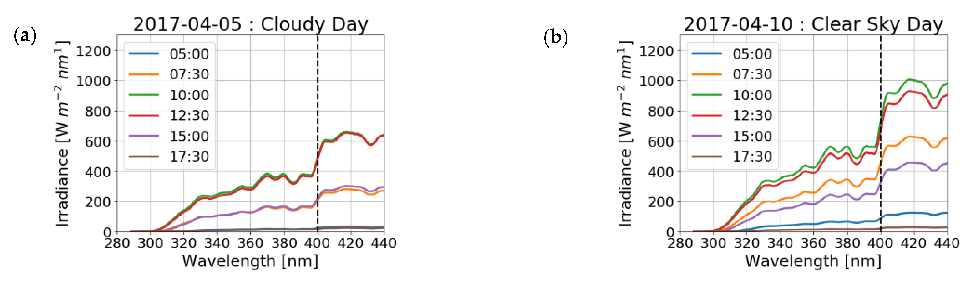
UV irradiance given in the ERA5 dataset covers a wavelength range up to 440 nm. However, this variable is usually referred for wavelengths below 400 nm. This distinction can cause large differences of the estimated UV irradiation. For example, measurements in Ljubljana, Slovenia lead to an overestimation of 45% of the energy in the UV part (see
Figure 1).
For this reason, we neglect the
irradiance data given by ERA5, and model it up to 400 nm using a method proposed in ref. [
26] and expressed in Equations (5)–(8), which is based on the clearness index (
) and the global horizontal irradiance (
). The
is calculated by dividing the
and the top-of-atmosphere irradiance extracted from ERA5. Unfortunately, the lack of valid measurements disallows that we validate the model worldwide.
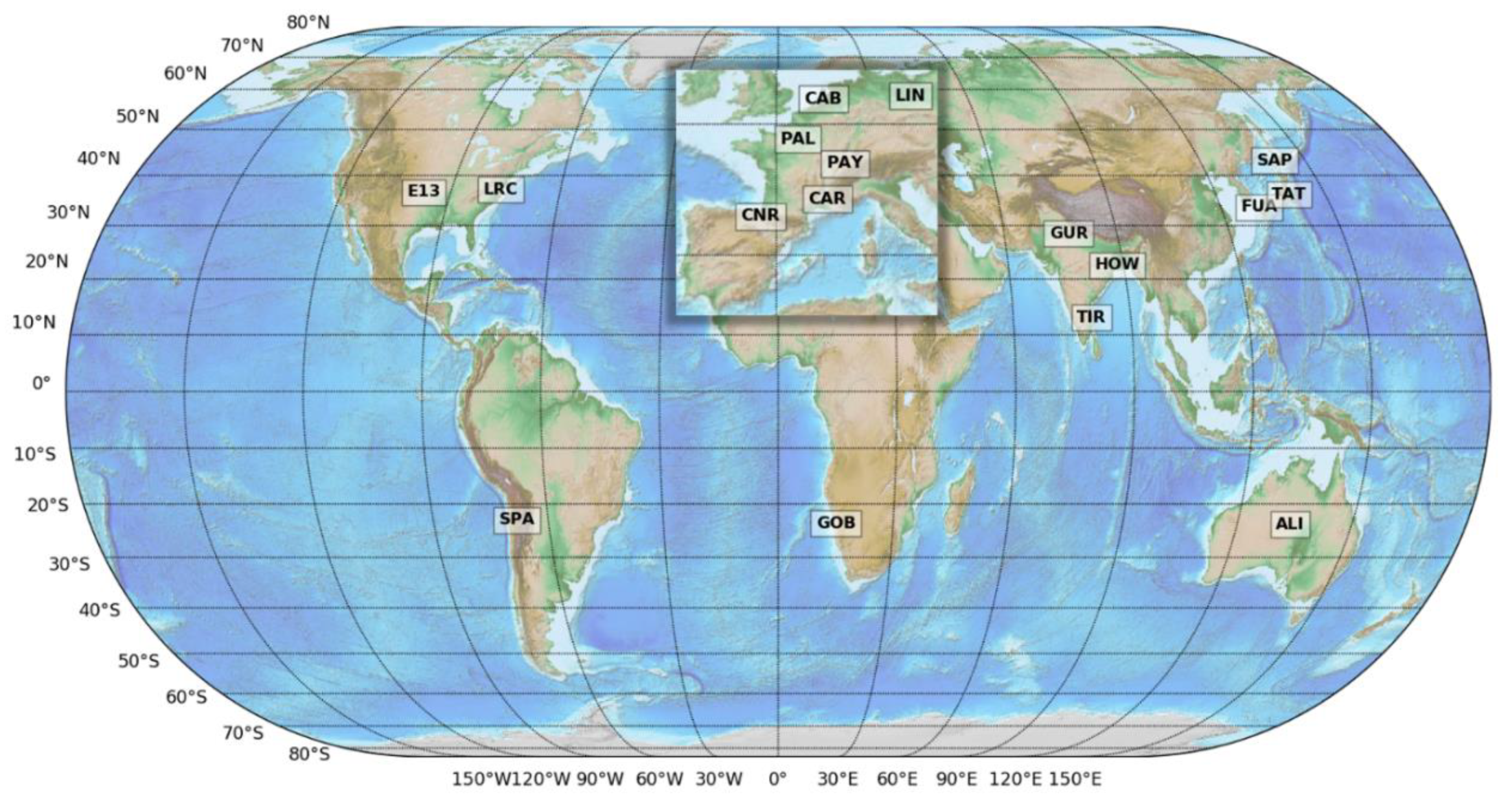
The GIS data extracted and computed is compared with 15 ground meteorological stations involved in the World Radiation Monitoring Center - Baseline Surface Radiation Network (WRMC-BSRN) [
17], one station in Alice Springs, Australia provided by the Desert Knowledge Australia (DKA) Solar Centre [
18] and one station in the Atacama Desert provided by Universidad de Chile [
19]. The station locations are shown in
Figure 2 and more details are presented in
Table A1 in the
Appendix A. At these stations,
,
, and
are measured. The comparison is carried out on a daily average resolution for the years 2016, 2017, and 2018, except for the Chilean station where the time frame ranges from 2010 to 2014. We use the inverse distance weighting (IDW) as interpolation method [
27] to calculate the estimated values at specific location reducing the geographical mismatch between measured and computed values.
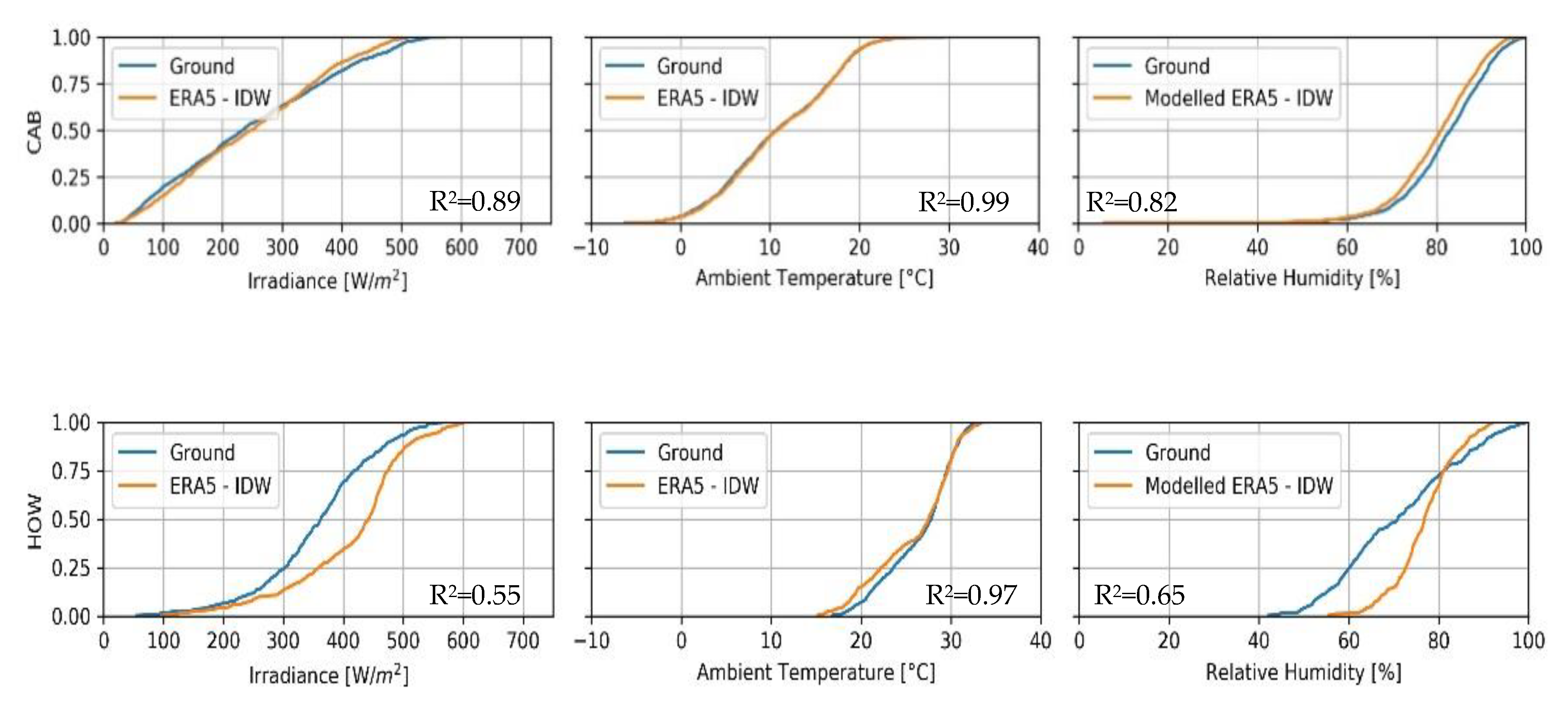
The time-series for each location are compared by the cumulative distribution function (CDF) and the coefficient-of-determination (R
2). In
Figure 3, locations with high and low accuracy are presented, while the rest of the locations are presented in
Table A2 in the
Appendix A. For example, on one hand, data in Cabauw (The Netherlands) show almost perfect fitting for the three variables (
,
, and
), evidencing that ERA5 can be used as synthetic data in some locations. On the other hand, in Howrah (India), the accuracy of
and
is low but could be improved with a post-processing algorithm, e.g., ref. [
28].
An excellent agreement of was noticed possibly because of the high number of observational data in ERA5. and also show good performance even though they are purely modelled.
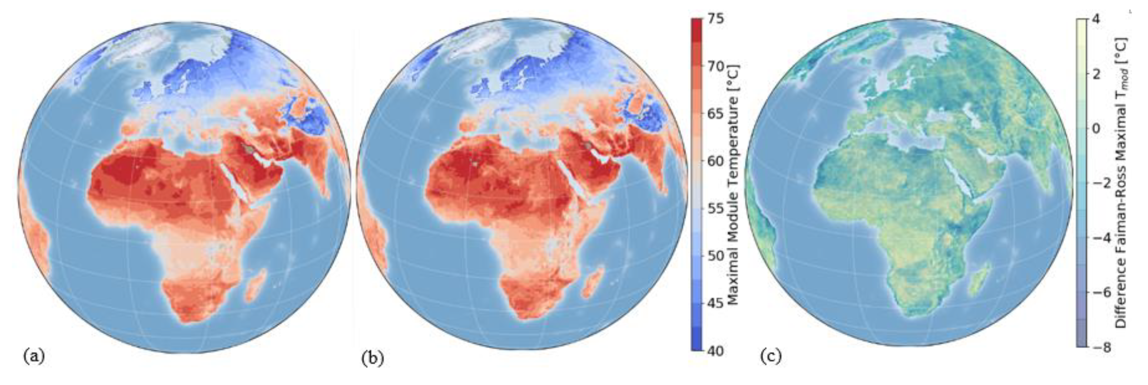
2.2. Operating Conditions of PV Modules
One of the most important climatic loads to analyze the degradation is the PV module temperature (
). Typically this variable is estimated by using the Ross model [
29], which is a function of the ambient temperature, irradiance and the Ross coefficient (
) as presented in Equation (9). However, a higher accuracy of
estimations under different climate conditions for crystalline silicon PV modules can be achieved by using the Faiman model (see Equation (10)) [
22,
30]. In
Figure 4, a visual comparison of the estimated
is illustrated. The main differences are presented in areas with high wind speed where the cooling effect will be taken into account when using the Faiman model.
Further calculations in this paper are based on the Faiman model to estimate the PV module temperature as a function of the
,
, and
, considering
equal to 26.9 W/m
2/°C and
equal to 6.2 Ws/m
3/°C [
23], which are typical values reported for c-Si PV modules in the open-rack mounting configuration.
3. Spatial Distribution of PV Degradation Rates
Degradation mechanisms will be triggered not only from one individual degradation factor but due to a combination of them. In ref. [
10], three degradation processes are defined and empirically expressed due to the combination of climate degradation factors: Hydrolysis-degradation (
related to the effect of temperature and humidity, photo-degradation (
) depends on temperature, humidity and UV irradiance, and thermo-mechanical-degradation (
) due to high temperature and temperature differences. The models are presented in Equations (11) to (14):
where the parameters are:
| : Hydrolysis degradation rate (%) | : effective relative humidity |
| : Photo-degradation rate (%) | : integral UV dose (kW/m²) |
| : Thermomechanical degradation rate (%) | : average module temperature |
| : Total degradation rate (%) | : upper module temperature |
| : Boltzmann constant (8.62 × 10⁻⁵) | : lower module temperature |
| : Activation Energy for Hydrolysis degradation (eV) | : temperature difference |
| : Activation Energy for Photo-degradation (eV) | : model parameter that indicates the impact of RH on power degradation. |
| : Activation Energy for Thermomechanical degradation (eV) | : model parameter that indicates the impact of UV dose on power degradation. |
| : Pre-exponential constant for Hydrolysis degradation | : model parameter that indicates the impact of on power degradation. |
| : Pre-exponential constant for Photo-degradation | : Cycling rate |
| : Pre-exponential constant for Thermomechanical degradation | : normalization constant of the physical quantities (a−2/%) |
The degradation mechanisms are quantified by using the fitting coefficients published in ref. [
10] for a high-performance monocrystalline silicon PV module installed in the open-rack mounting configuration.
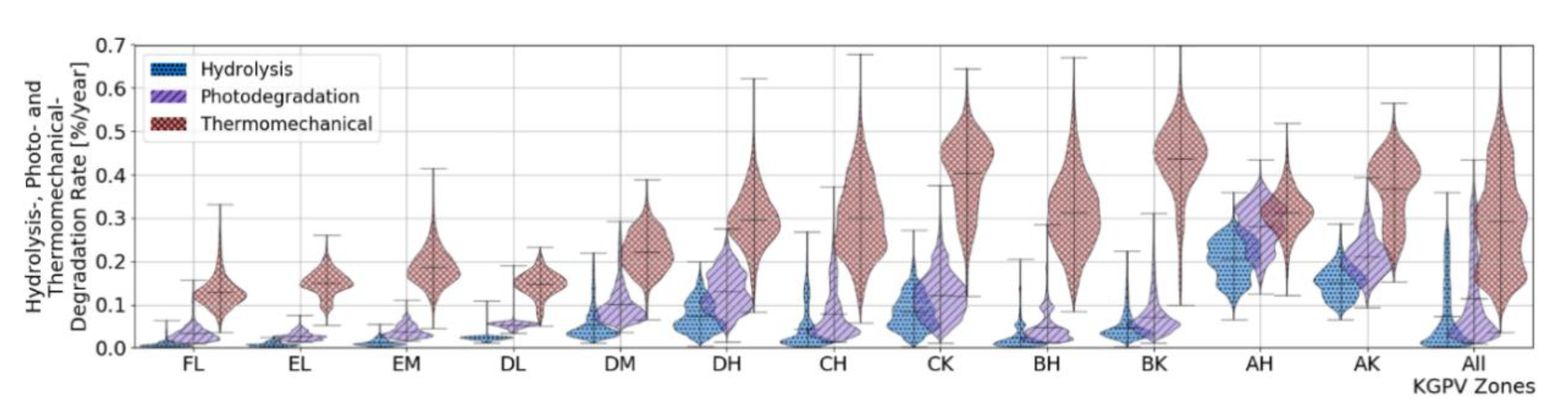
Further on, the calculated degradation rates can be directly related to climate zones. To simplify the spatial distribution analysis of degradation rates, we use the Köppen-Geiger-Photovoltaic (KGPV) scheme proposed in ref. [
12] to compare the climate zones in terms of annual degradation rates, as shown in
Figure 5 and
Figure 6. Each KGPV climate zone is defined by two letters, the first one implies the relation of temperature and precipitation (
TP-zones) and the second is related to the irradiation level, as
H-zones. The definition of each letter is as follows:
| Temperature-Precipitation (TP) Zones | Irradiation (H) Zones |
| : Tropical climate | : Very high irradiation |
| : Desert climate | : High irradiation |
| : Steppe climate | : Medium irradiation |
| : Temperate climate | : Low irradiation |
| : Cold climate | |
| : Polar climate | |
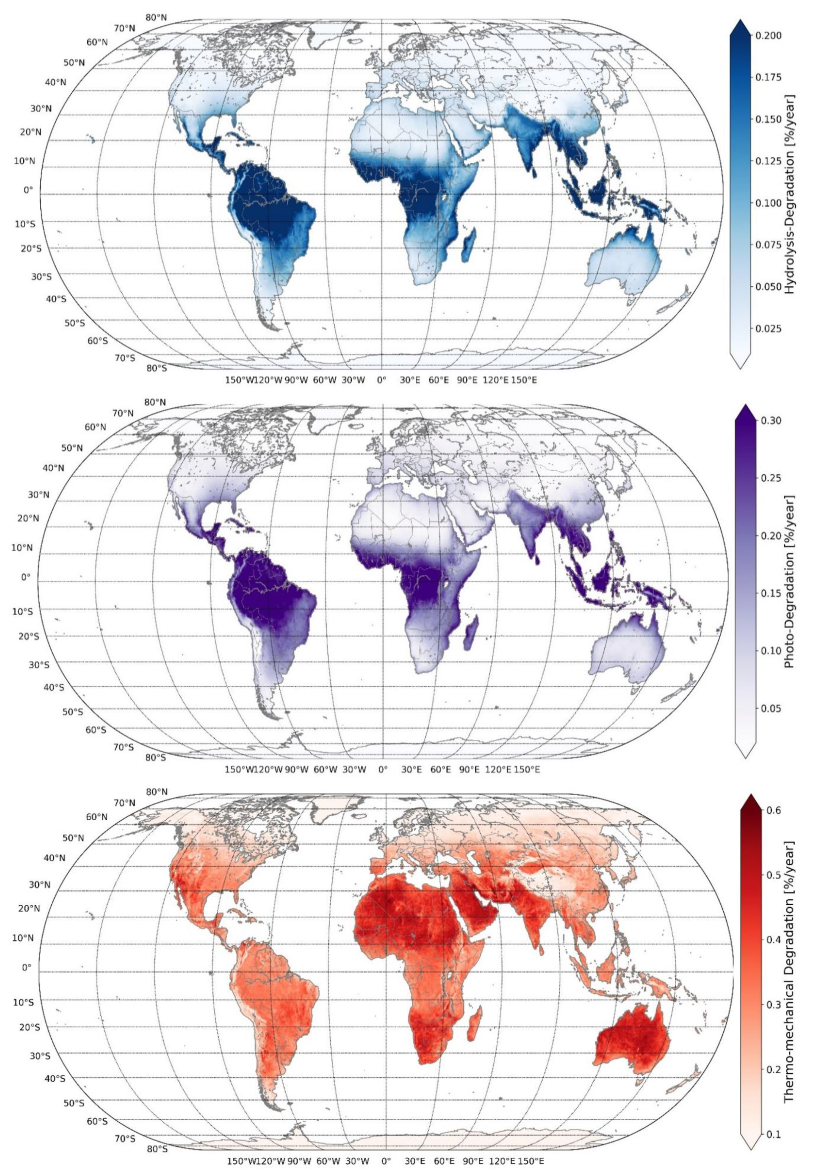
Hydrolysis-degradation presents the smallest contribution in almost all the KGPV zones, but is considerably higher for the tropical climates (AH and AK), which zones are related to high precipitation levels (humid areas) and temperature levels. This process can provoke moisture ingress leading to delamination of polymers or corrosion of solder bonds [
31].
Photo-degradation has the second-highest contribution to the total degradation rate. This indicator combines the humidity, temperature, and UV irradiance impacting the PV module. The impact is similar to hydrolysis-degradation but higher in terms of absolute values due to the process triggered by UV irradiation. For desert areas, even though the UV irradiation is high, the low humidity in the air decreases the estimated damage of the PV cells due to this mechanism. The photo-degradation is considerable high in tropical zones (AH and AK) due to the high climatic stresses of all variables (temperature, humidity, and UV irradiation).
Thermo-mechanical degradation exhibits the highest contribution to the total degradation rate in all zones, except in the AH zone, where the temperature variations are minimal. This parameter is affected by seasonal temperature cycling (the difference between the maximum and minimum temperature of the year) and also the annual average maximum ambient temperature.
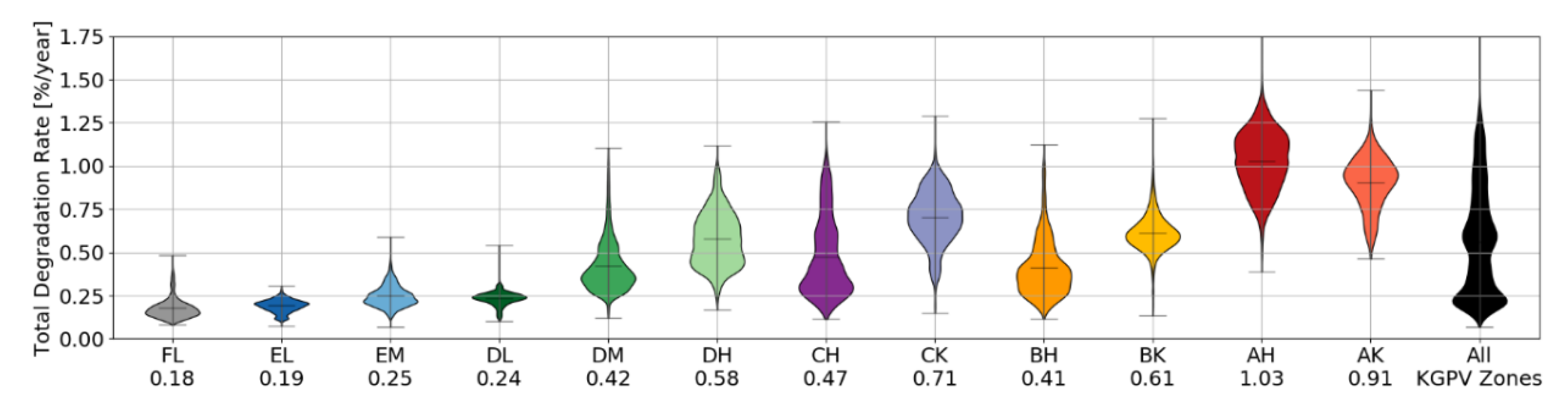
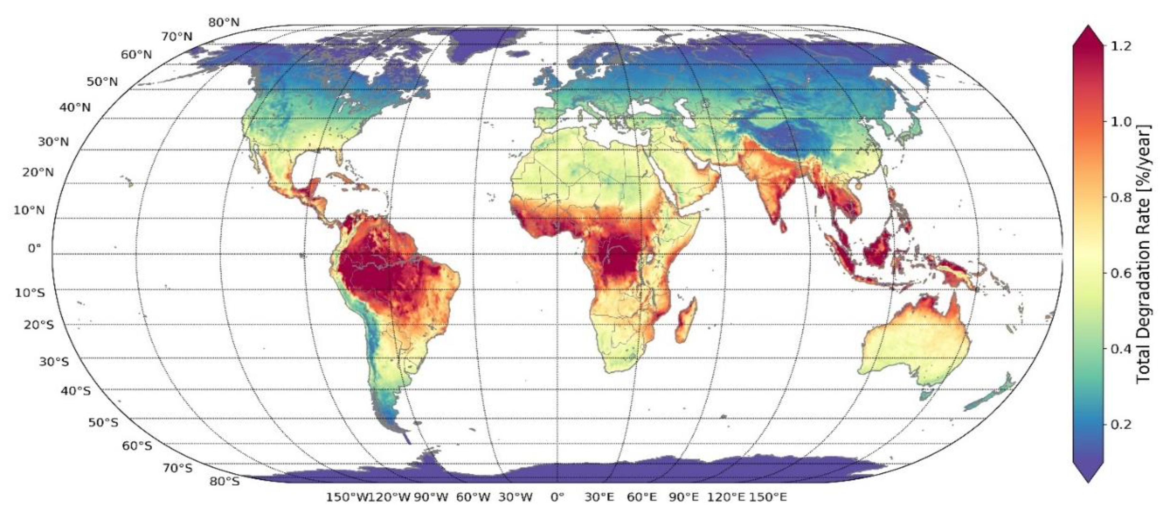
The total degradation rates calculated by the combination of the previous three degradation mechanisms Equation (13) are also evaluated per each KGPV climate zone. In accordance with the literature [
6], the highest degradation rate is identified in tropical areas (hot and humid). Interestingly, the AK (tropical with very high irradiation) presents lower degradation than the AH (tropical with high irradiation), due to lower photo-degradation contribution (related to lower humidity).
The steppe climate has higher humidity than the deserts and therefore, the total degradation rate is increased by higher hydrolysis-degradation and photo-degradation. As expected CK (steppe with very high irradiation) might be more stressful for PV modules than CH (steppe with high irradiation), due to higher UV irradiation.
Temperate climates (DM and DH) result in average degradation rates of 0.42%/a and 0.58%/a, respectively. Those climate zones are predominant in Europe, and their values are in accordance with the typical 0.5%/a degradation rate assumed along within the PV community. However, the spread of the values can range around ± 0.3%/a in the temperature zones across Europe.
Cold and polar areas present average degradation rates around or below 0.2%/a. In real operating conditions, we expect higher values due to external degradation factors, such as snow accumulation over the PV systems or mechanical loads due to wind gusts which are not included in the calculations as yet.
Desert areas exhibit similar average degradation rates than temperate areas. In absolute climate values, desert areas are hotter and dryer than temperate areas. However, in the relative contribution of degradation mechanisms, the high thermomechanical stress together with low hydrolysis and photo-degradation makes the average similar to the moderate climate stressors of the temperate climate. In real operating conditions, external degradation factors, such as soiling might increase the degradation rate if taken into account, but the degradation presented here assumes only gradual and non-reversible degradation processes.
4. Mapping of Degradation Mechanisms and Total Degradation Rate
The worldwide mapping of the degradation mechanisms (hydrolysis-degradation, photo-degradation and thermomechanical-degradation) are presented in
Figure A1 in the
Appendix B. As mentioned before, the simulations are based on the degradation model developed in ref. [
10], and coefficients fitted for a specific PV module (high-performance mono-crystalline silicon PV module). The climate datasets used were extracted, modelled and averaged from the ERA5 reanalysis dataset for the years 2016, 2017, and 2018.
Figure A2 in the
Appendix B shows the calculated worldwide degradation rate combining the three degradation mechanisms based on the main climate degradation factors.
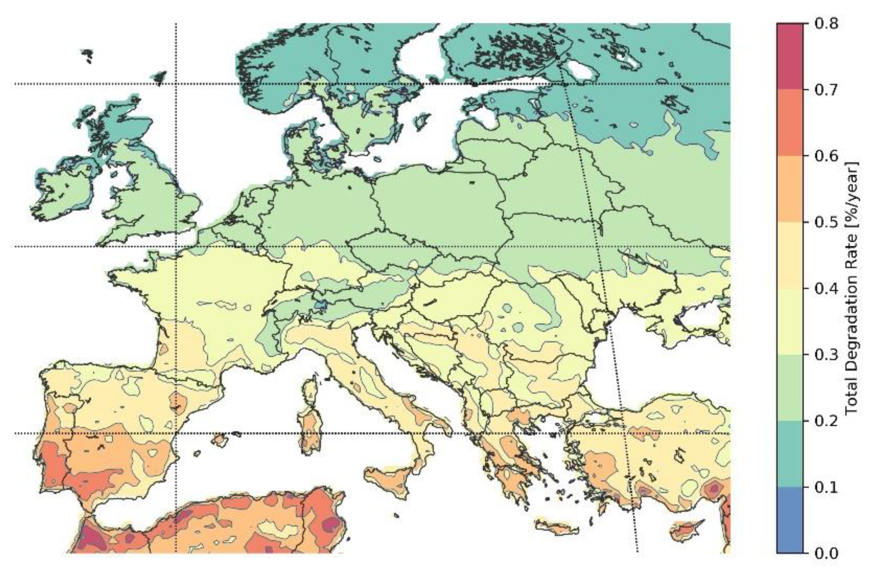
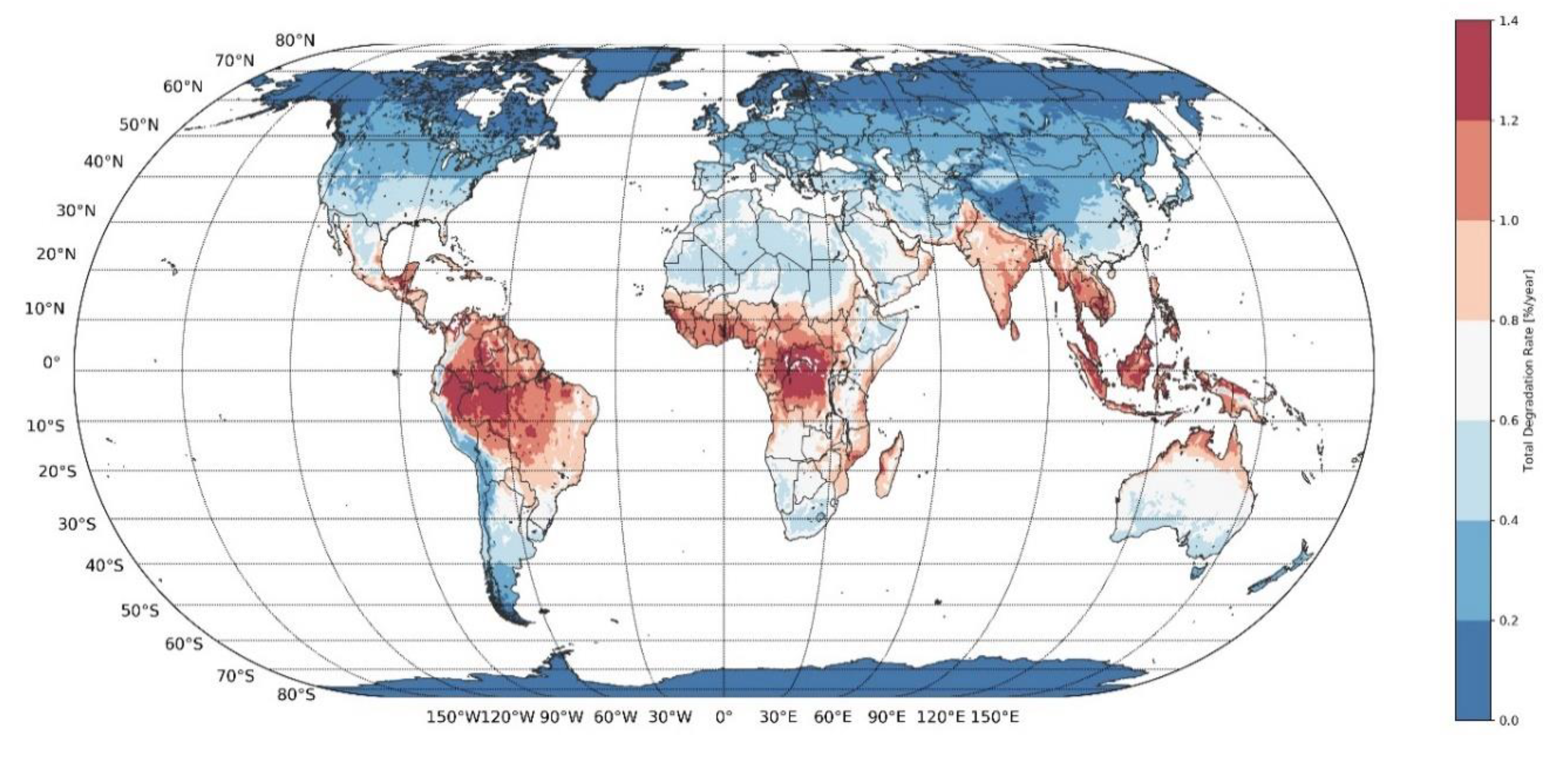
To facilitate the visualization and possible use of our degradation maps, we categorize the locations into bins of 0.2%/a ranging from 0% to 0.8%/a for Europe and ranging from 0% to 1.4%/a around the World. The categorized maps are shown in
Figure 7 and
Figure A3, respectively. The total degradation rates could reach 0.8%/a in the hottest areas of the south of Spain and Portugal for Europe, and globally the highest degradation rates (above 1.4%/a) are identified in locations next to the equator line.
5. Uncertainty over Time-Temporal Evolution
The temporal evolution of the climate also might be a factor to consider while estimating the degradation rates of PV modules. In ref. [
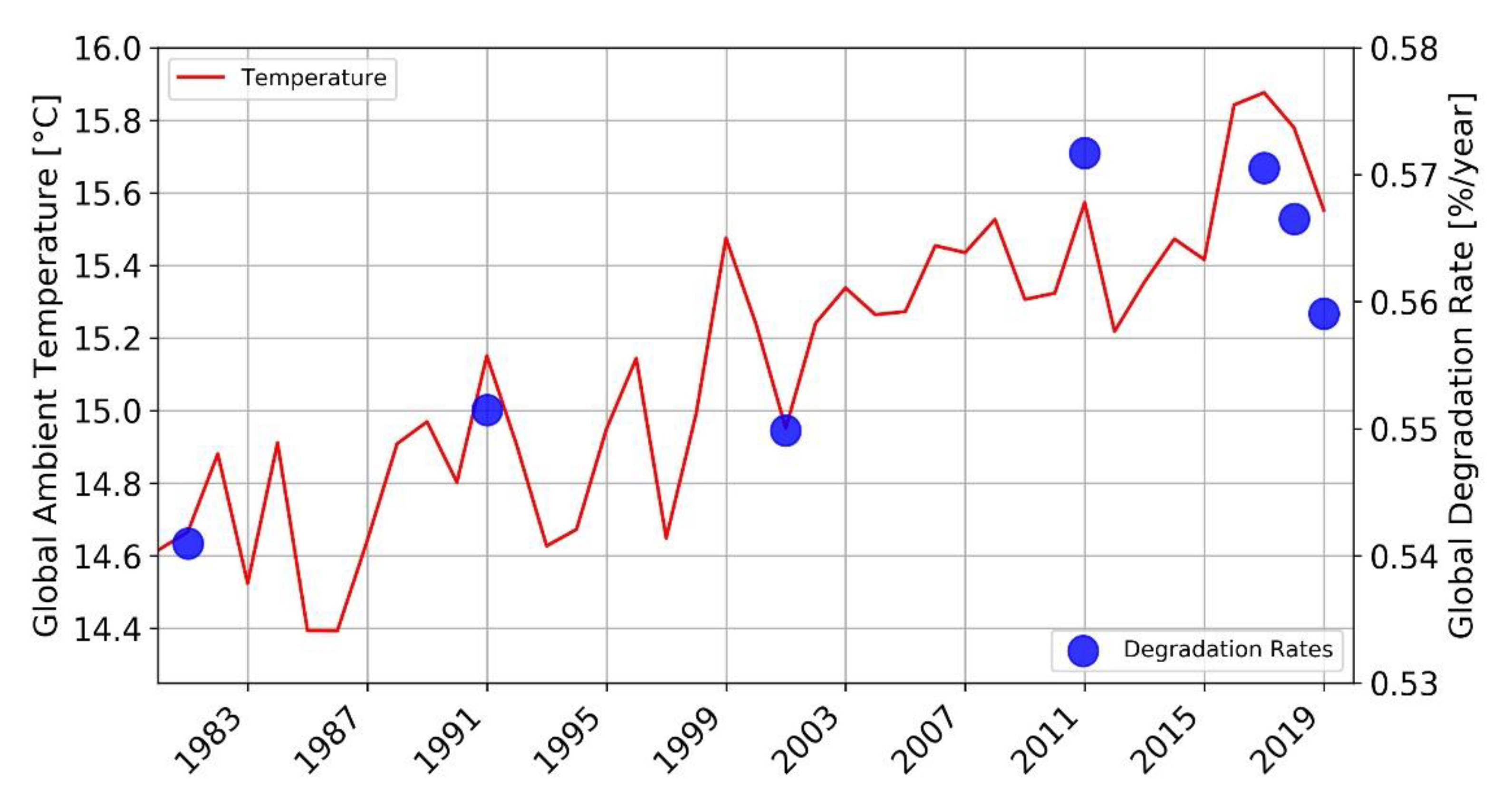
12] the decrease of the Performance Ratio due to climate change effect is already reported. Hereby, the annual degradation rates are simulated for the PV module described previously, using historical data from ERA5. For convenience in terms of computational resources, degradation rates based on hourly data are calculated only for the years 1980, 1990, 2000, 2010, 2016, 2017, and 2018. The ambient temperature is extracted for every year from 1979 to 2018.
In
Figure 8, the evolution of the ambient temperature and degradation rates is shown. The global calculations represent the average values for land-surface between the Latitudes −60° and 60°. We notice that an increase in the ambient temperature also increases the degradation of the PV modules over time.
6. Discussions
The used degradation model currently takes into account pure climate degradation factors and it does not include temporal or external degradation factors or failure modes such as light-induced degradation (LID), light and elevated temperature degradation (LeTID), potential-induced-degradation (PID) or mechanical damage due to wind or snow loads. Neither the underperformance due to soiling or snow covering is considered. Also, the final results of total degradation rates represent the value at steady conditions (for example, after LID). The calculations presented in this paper are related to a specific monocrystalline silicon PV module, and the values could be different for devices with different BOM but we expect the trend to remain the same for all crystalline silicon technologies.
The correlation with the KGPV climate zones shows a good agreement with the literature. Tropical climates are again presented as the harshest for PV modules due to the high humidity and high temperature. Desert and steppe climates present high degradation rates due to high daily temperature changes, even excluding soiling. Under no consideration of wind and snow loads, the temperate, cold and polar climates present low degradation rates.
Even though the results are coherent, some climate and degradation modelling topics need further investigation: (1) lack of UV irradiation measurements spread around the world does not allow a representative validation of models, (2) moisture ingress and related triggering of degradation processes, such as corrosion or delamination, need to be understood for different interactions of materials, and (3) the understanding of degradation mechanisms under high UV irradiance and extremely low humidity exposure.
Despite the current limitations, the average degradation rates calculated agree with the typical values used in manufacturer warranties and developers, showing that in the worst case (e.g., tropical climates) an average degradation of 1%/a can offer more than 20 years of performance above 80%, and the global average degradation rate of 0.5%/a could promise a lifetime operation of 40 years. Additionally, the mapping and results presented can give a new perspective of the climatic stresses worldwide when considering the installation of PV modules at different locations. Also, the high resolution of the GIS data, including ambient temperature, UV irradiation and humidity, together with the module operating temperature, helps to identify relevant variables for PV systems where measured data is not available. The degradation mechanisms and the total degradation rates calculated for the land-surface are available as
Supplementary Materials attached to this article.
7. Conclusions
In this paper, we used the ERA5 climate reanalysis dataset for the modelling of PV degradation mechanisms and total degradation rates worldwide. We demonstrated that by extracting the ambient and dew point temperature, the relative humidity can be estimated at any location. Also, by extracting the global and top-of-atmosphere irradiances, the ultraviolet irradiance was estimated. Then, the extracted and modelled variables (temperature, irradiance, and humidity) were combined to compute the degradation of PV modules in terms of photo-degradation, hydrolysis-degradation, and thermo-mechanical-degradation. The quantification of each degradation mechanism allowed us to estimate the total degradation rate globally for a specific monocrystalline silicon PV module.
To validate the estimation of climate variables, we extracted the time series of 17 ground measurement stations from the World Radiation Monitoring Center - Baseline Surface Radiation Network (WRMC-BSRN), Desert Knowledge Australia (DKA) Solar Centre, and Universidad de Chile which include ambient temperature, global horizontal irradiance and relative humidity. The cumulative distribution function and coefficient-of-determination (R2) were calculated to prove the good agreement between the ground measurements and the modelled data from ERA5 interpolated using the Inverse-Distance-Weighting method. For the validation, we considered daily average values from 2016 to 2018.
In terms of global spatial distribution, we found a clear correlation between the Köppen-Geiger-Photovoltaic (KGPV) climate classification and the estimated degradation rates. In the temperate zones of Europe, the average degradation rate is in accordance with the typical degradation rate of 0.5%/a considered widely by the PV community, however, this value can vary around ± 0.3%/a for a specific year.
From our calculations, thermomechanical degradation is the harshest for the studied PV module in nearly all climate zones, presenting the highest impact in very high irradiation zones, such as CK, BK, and AK. Photo-degradation and hydrolysis-degradation show similar global spatial distribution, but the former is higher since it also comprises UV irradiation as a degradation factor.
The temporal evolution of the degradation rates is directly correlated with the global ambient temperature and it is evidence that climate change could impact the long-term performance of PV systems.
We developed new maps for degradation mechanisms and the total degradation rate for the studied PV module which can be directly integrated as a new layer over the KGPV climate classification map and provide a rapid understanding of performance and degradation globally. However, due to the high uncertainty in the real degradation rate of PV systems (solar resource, methodology of calculation, quality of operational data, bill-of-materials of PV modules, etc.), the maps are presented as a guide to identify possible risk areas in terms of climate stress but not to give quantified degradation rates for specific locations for any PV module or PV system.

 ,
, 


