An Enhanced Two-Stage Grid-Connected Linear Parameter Varying Photovoltaic System Model for Frequency Support Strategy Evaluation

Abstract

Securing a future sustainable decarbonised economy involves moving towards a system with rising penetration levels of distributed photovoltaics (PVs) within the low voltage distribution network (LVDN). This power system evolution is displacing conventional generators and has resulted in a decline in inertia that is essential for frequency stability. Emerging network codes require PV generators to maintain a scheduled curtailed active power (CAP) reserve for under-frequency contingencies. In this paper, the development, verification and application of an enhanced, two-stage grid-connected, state-space, linear parameter varying (LPV) PV system model is presented. The LPV model provides accurate and efficient modelling for PV systems over the wide range of operating points associated with curtailed active power and is suitable for power systems with large numbers of distributed PV systems capable of frequency support in the LVDN, to be simulated within reasonable simulation times. In addition, the LPV model can be used to investigate voltage rise due to reverse active power. The model performance is evaluated using recorded experimental data with step changes in irradiation and active power curtailment. The measured data is generated from a power hardware in the loop (PHIL) testbed. The model’s performance is investigated on an adapted radial European LVDN benchmark with several distributed PV systems to present some of the challenges, opportunities and benefits. Step changes in solar irradiation are used to evaluate the dynamic behaviour of the LPV model compared to a discrete-time electromagnetic transient (EMT) model. A frequency droop control characteristic for frequency support is demonstrated. The results show a computational burden reduction of 132:1 compared to the EMT model and demonstrate the voltage rise due to reverse active power from providing frequency support during under-frequency contingencies.

1. Introduction

Electricity generation using low carbon technologies such as solar PV and wind turbine systems is beginning to play an essential part in achieving a sustainable decarbonised economy. Over the past decade, PV module prices have dropped by 79% leading to an exponential growth from a globally installed capacity of 6GW in 2006 to 638GW in 2019 [1,2,3]. In this transition, the existing electricity network is evolving towards a decentralised infrastructure with the decline of large fossil-fuelled conventional generators and the proliferation of millions of small geographically distributed PV systems, presenting multiple challenges to system operators [4]. One of the main challenges relates to the displacement of conventional synchronous generators that exhibit high inertia. As inertia decreases frequency stability also decreases, making the system response less robust to a disturbance [5].

With increased penetration of these renewable energy sources, they are very diverse and capable of providing grid support functionality needed to handle these challenges for frequency stability [4]. In order to allow maximum renewable generation in theory, it will be desirable for all renewable energy systems to provide grid support functionality. New controls incentivised by policy systems will be needed to maintain frequency stability [6,7].

Currently, PV systems operate at maximum power point (MPP) producing the maximum power available from the PV array using a maximum power point tracker (MPPT) controller. Frequency stability with declining system inertia can be maintained with the use of fast frequency support from renewable energy sources to slow the rate of change of frequency (RoCoF) and limit the frequency zenith/nadir during frequency transients [8]. In such scenarios with high penetration levels of renewable energy, various frequency support techniques can be implemented from wind turbines, energy storage systems (ESS) and PVs [7,9,10,11,12,13]. A typical PV system has no rotational inertia and minimal energy storage. Therefore, to provide grid support services in the form of active power curtailment for inertial and primary frequency support, the system must be capable of operating below its MPP. This also includes the capability of maintaining a curtailed active power reserve that can be dispatched during under frequency events [14,15,16]. In single-stage PV systems, curtailed active power reserves are achieved by enhancing the DC/AC converter control [15]. In two-stage PV systems, the DC/DC controller has to be adapted [17]. The curtailed active power reserve for primary frequency support is primarily delivered using a droop response (P(f) characteristic) and inertial response (IR) controller [17,18,19,20]. Alternative methods over size the DC-link capacitor and use it as an energy buffer [21], but this is still limited to short delivery times. At present, without any additional investment in ESS, it is more economically attractive for PV system enhancement to implement frequency support [21,22].

The evolution of the grid requires an evaluation of frequency support strategies with large numbers and high penetration of distributed PV systems feeding the LVDN as shown in Figure 1. This evaluation requires modelling of a large scale system with accurate analysis of voltage and active/reactive power control algorithms using smart PV systems [23]. The conventional approach for this analysis using a full EMT modelling approach for the PV systems would be very slow. An alternative approach to reduce computational resources and maintain accuracy for fast transient events is to model the PV systems with linear, average PV system models expressed in the dq0 reference frame [24,25,26,27]. Due to linear approximation of the highly nonlinear behaviour of the PV array generator [28] and step-up DC/DC converter [29] these models are only accurate in the region of the chosen linearisation point (normally maximum power point operation) for a specific irradiation and temperature. Operating points distant from the linearisation point are poorly represented by the linear model. Implementing grid support services in the PV system by curtailing active power results in the PV system operating point ranging over a wide array of values which cannot be represented accurately in a single linear model. In order to capture the nonlinear system behaviour over the wide operating range associated with frequency support services, a linear parameter varying (LPV) framework provides an attractive solution to represent a non-linear system as a combination of multiple linear models where at each instance in time a single LTI model is selected to describe the system behaviour [30].

This paper presents the development of an LPV PV system model to accurately capture the steady-state and dynamic response of a two-stage PV system capable of operating away from maximum power point (MPP) for under-frequency contingencies. To the author’s knowledge, this is the first presentation of an LPV model of a two-stage PV system. The development of an LPV model is significant for simulation-based investigations of large networks with multiple distributed PV systems that otherwise would be time-consuming and computationally expensive using detailed switching EMT models. The LPV model is an addition to previous work modelling a comprehensive linear state-space two-stage (LSS) PV system [27]. In that work, the PV system is linearised around a single equilibrium point at MPP, offering fast and accurate modelling. However, the LSS model is only valid for a very limited operating range with curtailed active power (CAP) near the equilibrium point of linearisation. In order to extend this operating range to anticipate the range required for frequency support services, multiple linear models are combined in the LPV model. The model is derived from an EMT model and both are validated using recorded experimental data for dynamic and steady-state performance at several solar irradiation intensities with an active power reserve. The recorded experimental data was created using a scaled PV system with a power hardware in the loop: real-time simulator (RTS).

The LPV PV system model is implemented on an altered radial European LVDN benchmark with low synchronous inertia to investigate the impact of declining system inertia and implement possible frequency support solutions [17,19]. The network is comprised of a steam turbine generator, eight network loads and seven 32 kWp distributed PV systems at each load centre to represent 100% penetration. Instead of using load perturbations [15,17,19,21], the effect of variable solar irradiation is used to assess the effectiveness of a droop controller response to offset adverse impacts at high penetration levels.

The development of the LPV PV system model, its validation with experimental data and its application in a distribution network are presented as follows. A description of the two-stage PV system under investigation is presented in Section 2. The development of the LPV model is described in Section 3. A comparison between the experimental measurements and the created LPV model are discussed in Section 4. In Section 5 the LV distribution network under investigation is described and the operation of the created LPV model is evaluated for both frequency response and voltage transients for various step changes in irradiation. The LPV model’s dynamic and steady-state response is compared with the full EMT model from which it is derived. The conclusions are outlined in Section 6.

2. PV System

The two-stage PV system under investigation is presented in Figure 2a. The system comprises of a PV array, step-up DC/DC converter, DC/AC converter, an LCL filter configuration and controllers. The red outlined section represents the PV system components and controllers derived as an equivalent state-space model in [27]. The PV array is represented by the equivalent single diode circuit model equations [31]. The instantaneous operating voltage of the array is used to solve the array current using iterative methods such as the Newton–Raphson method [32,33]. Grid support services for frequency support are implemented using the control structure, as shown in Figure 2b. At any time, the value of curtailed active power (CAP) $P_{cap}$ for power reserve can be a constant predefined by the network operator or dynamically updated as required. Based on the measured frequency, the frequency support controller (FSC) determines $P_{fs}$ which for under frequency is the portion of $P_{cap}$ delivered to the grid and for over frequency is the portion of $P_{cap}$ curtailed from maximum power point grid delivery. This results in an instantaneous curtailed active power for the PV system of $P_{ic}=P_{cap}-P_{fs}$. Based on this instantaneous curtailed active power, the active power reference for the PV system is $P_{ref}=P_{mpp}-P_{ic}$. The active power controller as shown Figure 2b can operate at MPP ($P_{mpp}$) or operate below MPP with an instantaneous curtailed active power. As the PV array power is a non-linear function of the operational voltage $v_{pv}$, it is difficult to predict the maximum power available at any instance, and when operating with a curtailed capacity, this can be achieved at voltages below and above the maximum power point voltage on the P-V curve. Also, this relationship continuously changes with variations in irradiance and panel temperature. Therefore, a PI controller regulating power is not effective as power does not increase linearly with duty cycle [14]. For this reason, the active power controller regulates the operating voltage $v_{pv}$ rather than power. Traditional maximum power point tracking methods such as perturb and observe (P&O) and incremental conductance (IC) do not require a measurement input of irradiation and temperature. To implement grid support services, as proposed in this work, it is essential to measure these meteorological parameters so alternative MPP techniques are considered. The approach adopted is to generate 2D look-up tables (LUTs) that use these measured inputs to determine the PV array maximum power $P_{mpp}$. A 3D LUT provides a voltage reference $v_{pvref}$ for the PV array [16]. The LUT method permits regulation of the PV array power to a given reference power $P_{ref}$. The maximum power available $P_{mpp}$ is calculated using a 2D LUT dependent on irradiation (G) and temperature (T). A 3D LUT provides a voltage reference $v_{pvref}$ for the PV array [16]. The reference voltage for the PV array $v_{pvref}$ is a function of the power reference $P_{ref}$, irradiation (G) and temperature (T). For operations other than the calculated points, the data is interpolated using trilinear interpolation. The LUT data is generated offline using the PV panel parameters from NREL System Advisor Model (SAM) [34] and solving the transcendental equation for a single PV panel over the expected operating space. The addition of panels in series or parallel changes the operating voltage $v_{pvref}$ ($v_{pvref}=v_{pvref}·N_s$) and the power reference $P_{ref}\left(P_{ref}=\frac{P_{ref}}{N_s·N_p}\right)$. In a physical implementation the 3D LUT and DC/DC controller will set PV operating voltage $v_{pvref}$. Continuous comparison of the modelled and measured PV array output power will allow the PV plant operator to identify faults and partial shading effects and notify the network operator. The model presented here does not implement this function and would also require further development to include partial shading effects.

2.1. PV System Modelling

In modelling the PV system there are several approaches that can be taken as shown in Figure 3. Each method has its own advantages and disadvantages related to simulation speed and accuracy. At the top level, the EMT model represents a component level system description that includes discrete switching devices that require the generation of PWM signals. In this work, these signals are generated at 10 kHz and require a 1 μs sampling time to provide a 1% duty cycle resolution. The system controllers use a 30 μs sampling time and data is recorded every 60 μs. The PHIL model uses a sampling time of 30 μs for both the controllers and the recording of data. In this case, the PWM signals are generated external to the simulation environment using a gate array. While the EMT model provides the most detailed information for comparison to the PHIL model, it imposes a large computational burden. In order to increase simulation speed and maintain a high level of accuracy, the switching device behaviour can be averaged over a switching period, creating an average model. This eliminates the need for a small sampling step time to generate the PWM signals and allows the use of variable step solvers that allow for increased sampling steps at steady-state operation. The computational burden can be further reduced by linearising the nonlinear average model. The linear model is time-invariant and is suitable for controller design, stability analysis and parametric sensitivity analysis and yields accurate results over a limited operating range near the equilibrium point [27]. This operating range is extended using the LPV model framework containing multiple linear models. In this work, the linear and LPV models are compared to the EMT model; the sampling time and data recording is reduced to 300 μs with a linear model sampling time of 3 ms which provides 27 samples in a step response of 80 ms for the PV system. The solvers are applied with both a maximum step size and relative tolerance of 0.003. The effect of different data logging sampling times used in the EMT model has an insignificant impact on simulation time.

2.2. PV System EMT Model

The developed EMT model of the three-phase PV system is shown in Figure 4. The model is used as the basis for derivation of the linear state-space PV system model’s differential equations and provides a reference for comparison. The parasitic losses related to non-ideal passive components are incorporated as resistor elements, derived from measurements and measured experimental data. The switching devices (IGBTs and diodes) are shown in red to display losses and are modelled as ideal switches with characterised losses depicted as a comparable voltage source [27].

3. LPV Model Development

In this section, an LPV model for the two-stage PV system is developed. The concept of LPV modelling is based on the traditional gain-scheduling framework [35]. In gain-scheduling, the non-linear system model is linearised at several operating points of interest resulting in a collection of local linear time-invariant (LTI) models. For each linear model, an LTI controller is designed. These controllers are then interpolated to create a global control solution for the non-linear system model [30]. The interpolation function is called the scheduling function and depends on the current operating point of the system. The changes in the operating point are described by an introduced signal called the scheduling signal ($\rho$). The parameters of the controller now depend on the varying scheduling signal. The controllers are now parameter varying.

Using the gain scheduling approach, an LPV model is created using the framework shown in Figure 5 by using a finite gridded domain of linear state-space models from several equilibrium points. Initially the LPV model is developed using the equivalent averaged time-invariant PV system differential Equations (1) and (2) in terms of z states $x(t)\in {\mathbb{R}}^z$, k inputs $u(t)\in {\mathbb{R}}^k$, q output measurements $y(t)\in {\mathbb{R}}^q$ related by n first-order state derivatives $\dot{x}$ for continuous-time systems, $t\in \mathbb{R}$ where $f_{pv}$ is the vector of PV system functions containing n differential equations, y is the system output measurements and h is the vector of output functions.

$$\dot{x}=f_{pv}(x,u)$$

(1)

$$y=h(x,u)$$

(2)

The linear time-invariant (LTI) state-space representation of (1) and (2) in continuous time is represented by (3) and (4) for $t\ge t_0$ and the initial conditions, $x(t_0)$, where A is the state matrix $A\in {\mathbb{R}}^{z\times z}$, B is the input matrix $B\in {\mathbb{R}}^{z\times k}$, C is the output matrix $C\in {\mathbb{R}}^{q\times z}$ and D is the feed-forward matrix $D\in {\mathbb{R}}^{q\times k}$.

$$\dot{x}(t)=Ax(t)+Bu(t)$$

(3)

$$y(t)=Cx(t)+Du(t)$$

(4)

The main advantage of using a linear parameter varying system $S(\rho )$ instead of an LTI system model is the ability to account for dynamic changes using a time-varying scheduling signal $\rho (t)$, this allows for system analysis and controller design subject to time-varying trajectories. The scheduling signal is a function $\rho =f(y,r)$ of the independent variables y and external signals r, this time variation is not known in advance but it is a measurable quantity at each instance in time. These independent variables are referred to as scheduling parameters. The LPV system is described as an array of parameter-dependent linear systems, whose state space representation depends on the scheduling parameters. The scheduling parameters are described as freely varying parameter values in the region P, $\rho \in \mathbb{P}$. The scheduling parameters chosen for the PV system are irradiation and instantaneous curtailed active power (G, $P_{ic}$), where $P_{ic}=P_{cap}-P_{fs}$. The LPV equivalent of a nonlinear system is presented in (5) and (6).

$$\dot{x}(t)=A(\rho (t))x(t)+B(\rho (t))u(t)$$

(5)

$$y(t)=C(\rho (t))x(t)+D(\rho (t))u(t)$$

(6)

3.1. Linearisation

The linear equations are obtained from the non-linear differential equations by using the first order terms of Taylor’s expansion series (7) [29] from an equilibrium point $(x_e,u_e)$ by solving each derivative of the vector $f_{pv}(x_e,u_e)=0$ where $x_e$ is the vector of equilibrium points for each state variable, $u_e$ is the vector of equilibrium points for each input, $(\delta u=u-u_e$, $\delta x=x-x_e)$ denotes the variation from the equilibrium points and $\nabla f_{pv}$ is the gradient of $f_{pv}$ evaluated at $(x_e,u_e)$.

$$f_{pv}(x,u)=f_{pv}(x_e,u_e)+\nabla f_{pv}{{|}_{(x_e{u}_e)}\delta x+\nabla f_{pv}|}_{(x_e{u}_e)}\delta u$$

(7)

Linearising the PV system about a single equilibrium point yields the linear state-space model (8) and (9), these linear models are used for the LPV framework as shown in Figure 6b:

$$\delta \dot{x}=A\delta x+B\delta u$$

(8)

$$\delta y=C\delta x+D\delta u,$$

(9)

where

$$\begin{array}{c}\hfill \delta y=y-y_e,A={\delta }_x{f}_{pv}(x_e,u_e),B={\delta }_x{f}_{pv}(x_e,u_e),C={\delta }_{x}h(x_e,u_e),D={\delta }_{x}h(x_e,u_e).\end{array}$$

The LPV model is created by using a finite gridded domain of linear state-space models from several equilibrium points $(x_e^i,u_e^i)$. The collection of LTI models describes the behaviour of the nonlinear system throughout the scheduling space P. Each model is a local approximation that describes the nonlinear system for small deviations. The entire set of LTI models $(x_e^i,u_e^i)\in P$ yields a linear parameter-dependent linearisation (${\rho }_e$). A regular grid is chosen to schedule between local LTI models, as shown in Figure 6b. The scheduling parameters’ irradiation and instantaneous curtailed active power (G, $P_{ic}$) define the local model.

3.2. Interpolation of Grid Points

For scheduling parameters of irradiation G and instantaneous curtailed active power $P_{ic}$ that are located on-grid locations, as shown in Figure 6a, the LTI model circled in blue best describes the operating dynamics at that instance. Using these scheduling parameters, a linear parameter-dependent system $S{\rho }_e$ is capable of locally describing the nonlinear model (10) and (11).

$$\delta \dot{x}=A({\rho }_e)\delta x+B({\rho }_e)\delta u$$

(10)

$$\delta y=C({\rho }_e)\delta x+D({\rho }_e)\delta u$$

(11)

When the scheduling parameter values ${\rho }_e$ are located off their grid locations as shown in Figure 6b, the scheduling function uses inverse distance weighted (IDW) interpolation of the 2$n_{\rho }$ nearest neighbouring LTI models in the scheduling space, where $n_{\rho }$ is the number of scheduling parameters. The nearest LTI models are obtained using the k-nearest neighbours (k-NN) algorithm by solving the Euclidean distance from the scheduled model ${\rho }_e$ as shown in Figure 6b. The IDW interpolation is based on the constant nodal function (12) where matrices $A_i$, $B_i$, $C_i$, $D_i$ are interpolated as weighted sums, $n_m$ is the number of nearest models ($n_m=2n_{\rho }$) and $w_i$ is the weight assigned to each $n_m$ LTI model. The inverse distance weighted method is influenced most by the nearest model and less by the more distant models. The total sum of the weights is equal to one (13). Weights are calculated using (14) where $h_i$ is the distance from the scheduled model to the weighting LTI model and $h_j$ is the distance from the scheduled model to the nearest $n_m$ LTI models.

$$A({\rho }_e)=\sum _{i=1}^{n_m}{w}_i{A}_i,B({\rho }_e)=\sum _{i=1}^{n_m}{w}_i{B}_i,C({\rho }_e)=\sum _{i=1}^{n_m}{w}_i{C}_i,D({\rho }_e)=\sum _{i=1}^{n_m}{w}_i{D}_i$$

(12)

$$\sum _{i=1}^{n_m}{w}_i=1,w_i\ge 0$$

(13)

$$w_i=\frac{h_i}{{\sum }_{j=1}^{n_m}{h}_j}$$

(14)

The LPV model is a family of LTI models linearised at various inputs of irradiation and reserve power (G, $P_{ic}$) so that each has their unique equilibrium points for states x, inputs u and outputs y that depend on these linearisation inputs. Taking this into account, the LPV model is extended to include the offsets in the state, input and output ($\dot{x}$, x, u and y) variables. Using the equilibrium offsets, the LPV model in (10) and (11) is represented by (15) and (16), which is an affine form of the LPV system:

$$\delta \dot{x}=A({\rho }_e)\delta x+B({\rho }_e)\delta u+[\delta \overline{\dot{x}}({\rho }_e)-A({\rho }_e)\delta \overline{x}({\rho }_e)-B({\rho }_e)\delta \overline{u}({\rho }_e)]$$

(15)

$$\delta y=C({\rho }_e)\delta x+D({\rho }_e)\delta u+[\delta \overline{y}({\rho }_e)-C({\rho }_e)\delta \overline{x}({\rho }_e)-D({\rho }_e)\delta \overline{u}({\rho }_e)],$$

(16)

where $\delta \overline{\dot{x}}({\rho }_e)$, $\delta \overline{x}({\rho }_e)$, $\delta \overline{u}({\rho }_e)$ and $\delta \overline{y}({\rho }_e)$ are offsets from the equilibrium points of irradiation and the instantaneous curtailed active power (G, $P_{ic}$) for $\dot{x}$, x, u and y at the scheduling function ${\rho }_e=f(G,P_{ic})$.

3.3. LPV PV System Model

The LPV PV system model is a linear system array approximation of the time average system dynamics. The PV system consists of a 1.25 kWp array made up of five series Conergy PH 250 Wp multi-crystalline panels. All PV system parameters are given in [27]. The PV system consists of 25 states and is considered to be of low complexity and can be efficiently solved without the need for truncation (the number of scheduling variables is at most 2 or 3 for this size system) [36].

The percentage error in output active power for a single LTI model linearised at 550 W/m² operating over the expected operating range with active power curtailment is shown in Figure 7 with a zoomed section over the operating range of 400– 1000W/m², this emphases how a single models accuracy varies with curtailed active power. The percentage error is calculated using (17) where $P_{EMT}$ is the output active power of a full EMT model, and $P_{LSS}$ is output active power of a single linear state space model. The single model remains accurate when operating off MPP within –3.2% to +0.5% in the range of 800–1000 W/m² with a curtailed capacity of 500 W (40%). While operating at 600 W/m² for the same curtailed capacity, an error of 16% exists and further increases as irradiation lowers. The operating range of the model can be extended by using multiple linear models linearised at various operating conditions.

$$P_{error}=\frac{P_{EMT}-P_{LSS}}{P_{EMT}}\times 100$$

(17)

As an example, Figure 8 shows the (P-V) characteristic curve evaluated at various irradiation levels at a constant temperature of 25 °C, MPP operation is highlighted on the knee of each curve by the dashed magenta line. The nonlinear curve for MPP voltage can be captured by using several linearised models. Three models linearised at [100, 550, 1000] W/m² using (7) are shown in Figure 9.

Increasing the number of linear models reduces the error highlighted in Figure 9 and provides a more accurate representation of output active power. Figure 10 shows how the percentage output error decreases for MPP operation using a total of up to 20 linear models, linearised in the range of 100 to 1000 W/m² with even spacing. A zoomed section over the operating range of 400–1000 W/m² shows that maximum error is 3% for a single model and the error rapidly decreases with just two models to 0.75%. In total, 10 linear models are chosen for changes in irradiance as the benefits above 10 models are minimal.

In order to capture the full operating envelope for this particular application, additional models are required for the inclusion of active power curtailment. Figure 11 shows how the PV array voltage varies for active power curtailment at 550 W/m² with a constant temperature of 25 °C. Depending on the irradiation level and active power curtailment, the operating range of the PV array varies widely, making it difficult for a single scheduling parameter to capture the expected operational range as shown in Figure 12.

Increasing the number of linear models for active power curtailment is shown in Figure 13 for a constant irradiance of 550W/m². This shows how the percentage output active power error decreases with an increasing number of linear models. The percentage error of the LPV model is calculated using (18) where $P_{LPV}$ is output active power of the LPV model. For active power curtailment, the maximum error in output active power decreases rapidly with an increasing number of models from 54.8% for a single model to 5.6% for two models and 0.2% for six models with an active power curtailment in the range of 0–500W. The zoomed section in Figure 13 shows how rapid the error decreases when using three or more models with a curtailed capacity in the range of 0–500W. From these results, six linear models are chosen to capture the PV systems’ operating points when operating off MPP in the range of 0–500W.

$$P_{errorlpv}=\frac{P_{EMT}-P_{LPV}}{P_{EMT}}\times 100$$

(18)

A combination of linear models for irradiation and active power curtailment is shown in Figure 14 for constant irradiation of 550 W/m² with a fixed number of six linear models for active power curtailment. For irradiation, various numbers of linear models are chosen (1, 2, 5, 10, 60), this gives a maximum combination of 120 linear models. The difference in simulation time from a single model to 120 models is small, and the most significant constraint in expanding the number of models applied is model generation time. From these results, considering model generation and accuracy, 60 linear state-space models were chosen for use with a regular grid, as shown in Figure 6. The scheduling parameter values irradiation G and instantaneous curtailed active power $P_{ic}$ consist of 10 and six values, respectively. The gridded array contains a linear state-space model at every combination of G and $P_{ic}$.

4. Model Validation

An experimental hardware testbed (EHT) as shown in Figure 15 was built to assess the EMT and LPV models. The measured experimental data is compared against the LPV model for dynamic and steady-state response. The testbed was built to emulate a scaled PV system with a power rating of 1.25kWp. All system parameters remain the same for both the EMT and EHT models as described in [27].

Results

The results in this section are used to assess the accuracy of the developed LPV model against an experimental hardware testbed, a single linear state-space (LSS) model linearised at 500 W/m² with 0 W curtailed and a full EMT switching PV system model simulated in MATLAB. All models receive step changes in irradiation, as shown in Figure 16 with a constant temperature profile. An active power curtailment of 300 W with unity power factor ($Q_{ref}=0\mathrm{VAr}$) is applied at 3.5 s to demonstrate the capability of active power curtailment for frequency support. The power curtailment is achieved by making the PV array operating voltage exceed the MPP voltage, as shown in Figure 17 where $v_{pvref}$ is the reference voltage to achieve active power curtailment and $v_{pvrefmpp}$ is the reference voltage for maximum power point operation. Operating at the right-hand side of the P-V curve in this way is preferred for improved dynamic performance, increased converter efficiency and controller robustness [14].

The active power extracted from the PV array is shown in Figure 18. All models generate similar steady-state operating values for PV array power as the PV array uses the equivalent single diode circuit model equations [31] and solves for array current based on the instantaneous operating voltage [32,33]. The active power output for all models is shown in Figure 19. Once operating off MPP with a reserve of 300 W the accuracy of the LSS model starts to decline as the irradiation decreases. The LSS model is unable to capture the full operation of the PV system with an active power reserve. The LPV model produces similar dynamics and steady-state operation for various irradiances with active power curtailment when compared to both the measured experimental data and EMT model. This validates the capability of the LPV model to capture the entire operation of a PV system for active power curtailment.

When operating at MPP, the duty cycle of the step-up DC/DC varies non-linearly by 2.15% as shown in Figure 20. As with Figure 9, the linearised model accuracy can be improved by including several linear models with three models linearised at (100, 550, 1000) W/m² as shown in Figure 20. Operating with a curtailed active power as required for GSS, the duty cycle has a broader range of nonlinear variation of 7.8%, as shown in Figure 21. The data for CAP 0 W is the same as Figure 20 while the effect of increasing levels of active power curtailment results in the high variation in duty cycle. The DC/AC converter for the same operation presents a linear relationship between the duty cycle and the output active power for control of both active and reactive power as shown in Figure 22 and Figure 23 respectively. These results show the non-linearity of the DC/DC step-up converter duty cycle variation over the full irradiation range and indicate that this may result in significant steady-state errors in a linearised model.

5. Network Simulations

The purpose of the developed LPV PV system model was to enable system-level simulations and its usefulness was tested on a radial LVDN. Two different scenarios are investigated:

• Maximum power point tracker (MPPT) operation with no frequency support provided.
• A P(f) droop characteristic for frequency support.

The results are validated against a full EMT model of the LVDN. The network disturbance considered focuses on the impact of variations in solar irradiation and all loads remain constant. Step changes in solar irradiation are used for dynamic performance characterisation. Two irradiation profiles are used, as shown in Figure 24 and Figure 25 for over and under frequency events. The temperature profile of the PV array is constant for all analyses (25 °C).

5.1. Three-Phase Network Description

The impact of increasing PV system penetration is analysed on a modified radial, 20 nodes symmetrical three-phase commercial CIGRE European LVDN benchmark [37]. The network consists of seven distributed load centres totalling 217.8 kW. The LVDN is modified by including a steam turbine generator and by adding seven PV systems (7 × 32 kW) at each distributed load centre to represent 100% penetration. The modified one-line diagram of the European LVDN is shown in Figure 26. The detailed parameters of the distribution line are given in

Table 1. Network parameters.

Conductor	Size	R at 50 °C	X	Length
ID	mm2	Ω/km	Ω/km	m
OH1	19 × 70 mm2	0.491	0.2716	60
OH2	7 × 25 mm2	1.320	0.3066	60
OH3	7 × 16 mm2	2.016	0.3197	60

[37]. As the lengths of the distribution lines are short, the capacitance is small and considered negligible.

The LVDN is modified by replacing the slack bus with a steam turbine generator, as shown in Figure 26. This provides a controllable system with a realistic performance for low inertia networks, allowing for the evaluation of high penetrations of PV with and without frequency support strategies on frequency dynamics. Since frequency dynamics are the primary objective, a single synchronous generator provides the full operating range of loads.

The electrical generator in this study is described by a sixth-order dq state-space model. The model takes into account the field circuit and a single equivalent damper winding [38]. A steam turbine is used to represent the prime mover without a reheat steam turbine as shown in Figure 27 and governor based on TGOV1 [39,40]. The model is characterised by the steam turbine, the main steam control valve and the control valve limits ($V_{max}$ and $V_{min}$). The steam turbine and the main steam control valve are described by first-order transfer functions with time constants $T_{tur}$ and $T_{va}$ respectively. The governor regulates the turbine’s mechanical power ($P_{mac}$) into the synchronous generator based on the combined angular velocity (ω_m) and the generator power set-point ($P_{gensetpoint}$) with droop characteristic ($R_{droop}$). The droop characteristic provides primary frequency support speed regulation allowing for even generator load sharing based on each generators reference. A 4% droop characteristic is chosen as the default [41]. Restoration of the system frequency to the nominal value of 50 Hz after an event causing an increase or decrease in load requires a supplementary control action in the form of a secondary controller that adjusts the generator power set-point $P_{gensetpoint}$ from the scheduled power $P_{sch}$. The automatic generator controller (AGC) is initiated 30 s after a frequency excursion outside the controller limits as shown in Figure 27. As the secondary frequency controller is not the focus of this work, an additional integral controller is added to speed up system restoration when the frequency is below 50.1 Hz or above 49.9 Hz after a frequency excursion. This addition controller reduces the overall time window for which the simulation must be run to demonstrate the various responses. Typically, primary frequency control responds within 30 s and secondary frequency control responds in a range of 5 s up to 10 minutes after the change in frequency [41].

The generator’s terminal voltage is regulated using a static excitation system based on an IEEE Type ST1C voltage source [42,43] rectifier exciter as shown in Figure 28 with limited exciter voltage ($V_{amax}$ and $V_{amin}$). The voltage regulator gain and the excitation system time constant are expressed by $K_a$ and $T_a$, respectively. The transient gain of the system is reduced by implementing a feedback gain expressed by the rate feedback gain ($K_f$) and the rate feedback time constant ($T_f$). Parameter values are given in p.u. in

Table 2. Network generator parameters.

Paramater	Value	Paramater	Value	Paramater	Value
$T_{va}$	5ms	$T_{tur}$	0.5s	$k_i^{gov}$	0.58
$k_p^{gov}$	2.62	$k_i^{s2}$	0.075	$T_f$	20ms
$T_a$	1ms	$k_a$	350	$k_f$	1ms
$k_i^{s1}$	0.025

.

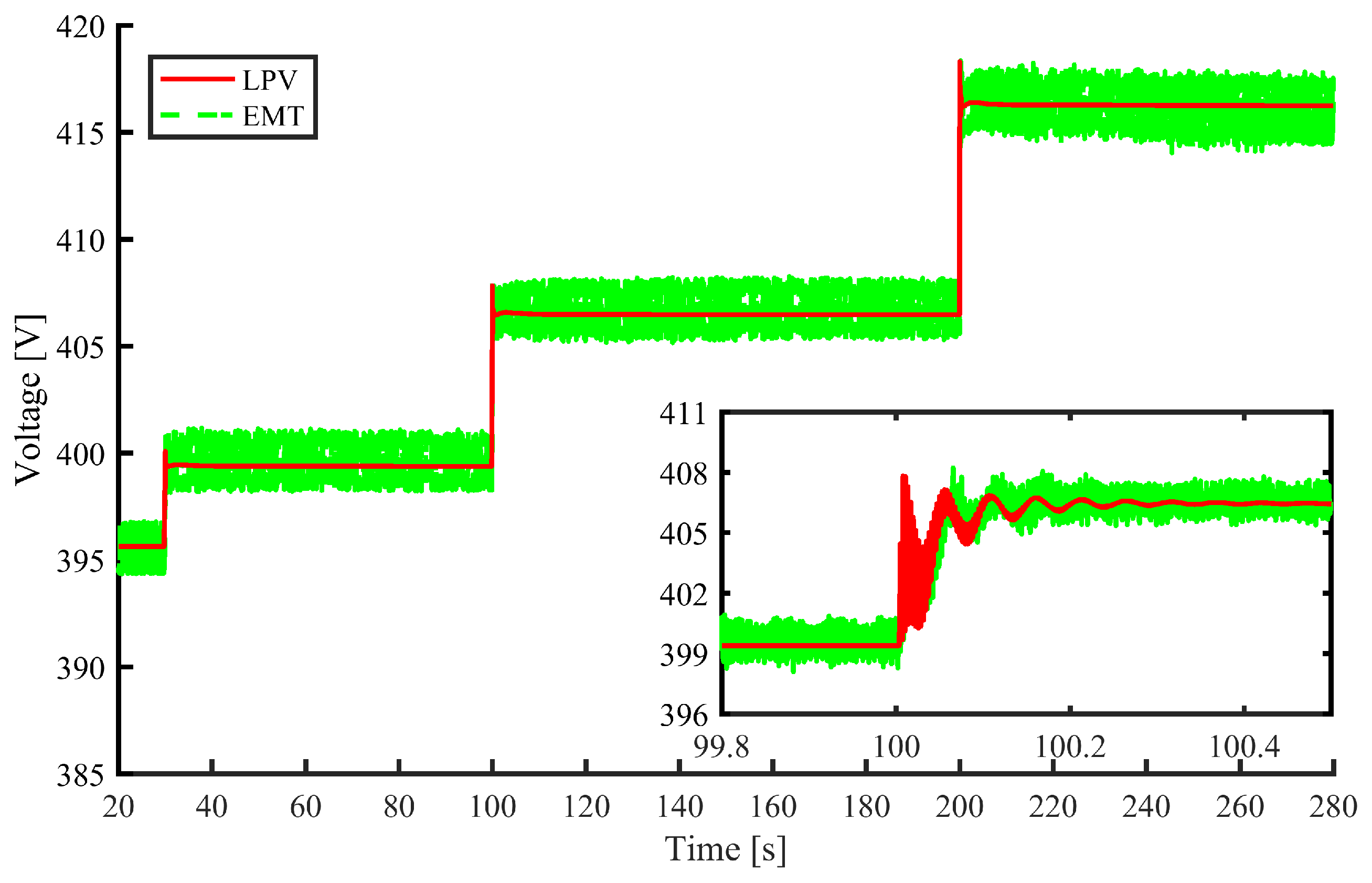
5.2. Response to Increasing Solar Irradiation

The LPV model’s accuracy for over frequency events is evaluated in this section. The step changes in solar irradiation that increase generation by 10, 20 and 30% of rated capacity at constant temperature are shown in Figure 24. The droop characteristic for over frequency events is in the range of 50.2 to 51 Hz (1.6% droop). If the frequency is higher than 51 Hz the PV system fully curtails active power generation.

The system frequency response for the PV with an MPPT controller only and no frequency support is shown in Figure 29. When the PV systems are operating with an MPPT controller, the objective is to deliver as much active power as possible. Since each PV system has a fast dynamic response, the generator is unable to respond quickly enough to balance the system active power demand causing the frequency to rise. As a result, a maximum frequency excursion of 53.9 Hz and a RoCoF of 2.4 Hz/s occurs (exceeding rated limits) for a sudden increase of generation equivalent to 30% of capacity.

The system frequency response for the droop controller is shown in Figure 30. The implementation of droop control alone from each PV system provides sufficient frequency support by maintaining frequency within limits, reducing the maximum frequency deviation by 79% (53.9 to 50.8Hz). Using the droop controller does not reduce the initial RoCoF.

The voltage at bus 17 is measured to assess model accuracy and voltage rise due to increasing solar irradiation. Bus 17 is chosen due to the distance from the generator and low local load to demonstrate worst-case voltage rise due to reverse active power flow. The voltage at bus 1 is regulated to 400 V. The voltage at bus 17 is shown in Figure 31 and Figure 32 for MPPT and droop control respectively. As solar irradiation increases, PV active power generation becomes larger than local load demand resulting in reverse-active power flow, causing voltage rise. The sudden increase in voltage rise in Figure 31 and Figure 32 is due to the step increase in solar irradiation and the fast response of the PV system. The transient response in Figure 32 is due to the droop controller working from a feedback loop using frequency. The event occurs before the controller responds, and active power cannot be curtailed until frequency increases. It can be seen in Figure 32 that the voltage settles briefly before active power is curtailed. Perhaps a Q(f) or P(Q) characteristic dependent on RoCoF could limit these voltage transients [44].

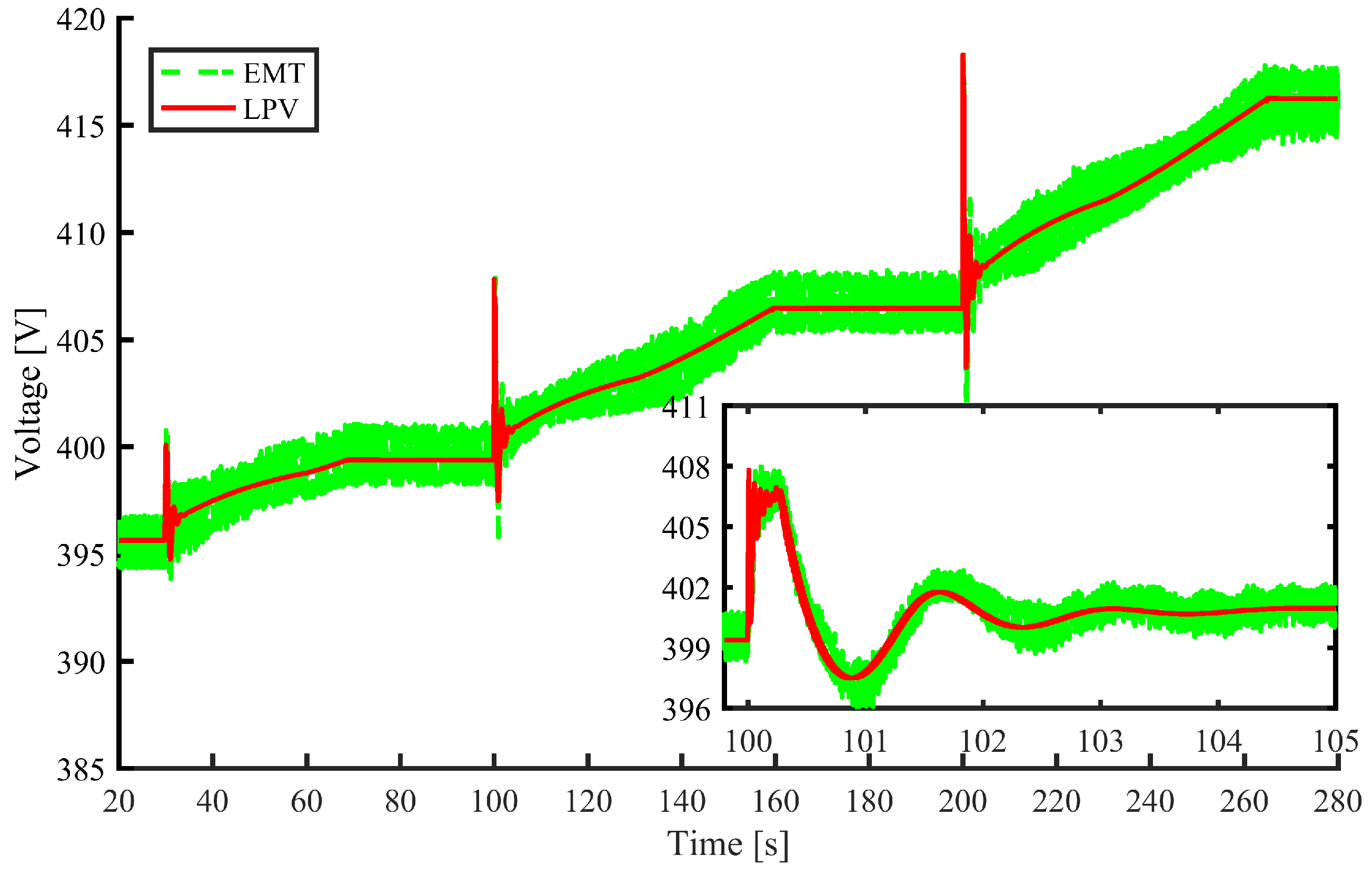
5.3. Response to Decreasing Solar Irradiation with Active Power Reserves

The LPV model’s accuracy for under frequency events is evaluated in this section. The output is compared against an EMT model for step changes in irradiance. The step changes in solar irradiation decrease generation by 10, 20 and 30% for a constant temperature using the irradiation profile as shown in Figure 25. The droop characteristic of under frequency events is in the range of 49.8 Hz to 49 Hz (1.6% droop). If the frequency is less than or equal to 49 Hz, the PV system operates at maximum power. Once system frequency is above 49.8 Hz, all PV systems operate with the specified curtailed active power reserve of 16% for the droop controller.

The system frequency response for the PV with an MPPT controller only and no frequency support is shown in Figure 33. When each PV system operates with an MPPT, the maximum frequency deviation is 4.5 Hz, and a RoCoF of 2.77 Hz/s occurs for a sudden loss of PV generation equivalent to 30%.

The system frequency response for the droop controller is shown in Figure 34. For a sudden loss of PV generation equivalent to an imbalance of 30% with each PV system operating with a droop controller, the maximum frequency deviation is 2.24 Hz which is a 50.22% reduction compared to MPPT operation. The droop controller, however, does not reduce the system RoCoF.

The loss of PV generation due to decreasing irradiation causes bus voltage to fall. The voltage at bus 17 is shown in Figure 35 and Figure 36. Without frequency support from each PV system, the voltage at bus 17 falls nearly instantly for each step decrease in solar irradiation. The implementation of the droop controller dampens the fall in voltage by delivering active power locally from an active power reserve. Active power plays an essential role in voltage regulation, where the network line’s R/X ratios are high; this is especially true for LVDNs. The voltage profile at each bus can also be further improved by implementing a Q(V) droop controller offsetting the reactive component [45].

In summary, the results presented in this section show the validation of the LPV PV model for frequency support investigation and the potential of frequency support control with low synchronous inertia systems. The model was validated by comparing the dynamic performance with a full EMT switching model in MATLAB, as shown in Figure 29, Figure 30, Figure 31, Figure 32, Figure 33, Figure 34, Figure 35 and Figure 36. From these time-domain simulations, the dynamic behaviour was assessed using system frequency and bus voltage. The LPV and EMT PV system models produce similar system responses and steady-state values for both increasing and decreasing step changes in irradiation with frequency support controllers. A summary of the simulation times and computational burden reduction between the EMT, average and LPV model is shown in Figure 37. The simulation time on average was reduced by 99.2%, from 37 h to 0.28 h; this is a computational burden reduction of 132:1 between the EMT and LPV model. These results demonstrate the benefits of the LPV PV model when investigating a high penetration of distributed PV systems in a large scale distribution network. Another advantage of this model is the ability to investigate bus voltage, which could violate voltage limits due to reverse active power when providing active power to support frequency.

6. Conclusions

In this paper, a linear parameter varying (LPV) model of a two-stage grid-connected PV system was introduced with flexible active power control for frequency support. The model builds on previously published work [27] to formulate a fast and accurate model, suitable for power system studies with increasing penetration levels of PV. The function of the LPV model is to accurately capture the non-linear behaviour of a two-stage PV system over the wide range of operating points associated with curtailed active power for GSS. The LPV model is validated with curtailed active power using recorded data from an experimental hardware testbed (EHT). The dynamic and steady-state performance at multiple emulated step changes in irradiation is assessed. The potential of the LPV model and the effectiveness frequency support using a P(f) droop control for PV systems were simulated on a 20 node isolated modified European LVDN with low synchronous inertia and compared against a full EMT switching model. These simulations demonstrate that the LPV model can emulate the behaviour of an EMT model with comparable dynamics and steady-state running values with a reduction in simulation time by 132:1.

References

1. Sawin, J.L.; Seyboth, K.; Sverrisson, F.; Rana, A.; Murdock, H.E.; Fabiani, A.; Adam, B. Renewables 2017 global status report. In Advancing the Global Renewable Energy Transition; REN21: Paris, France, 2017; p. 45. [Google Scholar]
2. SolarPower Europe. Global Market Outlook For Solar Power: 2018–2022. Available online: http://www.solarpowereurope.org (accessed on 21 February 2019).
3. McCrone, A. Clean Energy’s Decade Nearly Gone, and Its Decade Ahead. BloombergNEF. 2019. Available online: https://about.bnef.com (accessed on 31 October 2019).
4. Kroposki, B.; Johnson, B.; Zhang, Y.; Gevorgian, V.; Denholm, P.; Hodge, B.M.; Hannegan, B. Achieving a 100% Renewable Grid: Operating Electric Power Systems with Extremely High Levels of Variable Renewable Energy. IEEE Power Energy Mag. 2017, 15, 61–73. [Google Scholar] [CrossRef]
5. Tielens, P.; Van Hertem, D. The relevance of inertia in power systems. Renew. Sustain. Energy Rev. 2016, 55, 999–1009. [Google Scholar] [CrossRef]
6. REserviceS. Economic Grid Support Services by Wind and Solar PV. Available online: https://www.reservices-project.eu/wp-content/uploads/REserviceS-authors-correction.pdf (accessed on 1 September 2019).
7. Rahmann, C.; Castillo, A. Fast frequency response capability of photovoltaic power plants: The necessity of new grid requirements and definitions. Energies 2014, 10, 6306–6322. [Google Scholar] [CrossRef]
8. EirGrid and SoNi. RoCoF Alternative & Complementary Solutions Project. Available online: http://www.eirgridgroup.com/site-files/library/EirGrid/DS3-RoCoF-Alternatives-Solutions-Project-Phase-2-Overview-Final.pdf (accessed on 1 September 2019).
9. Delille, G.; François, B.; Malarange, G. Dynamic frequency control support by energy storage to reduce the impact of wind and solar generation on isolated power system’s inertia. IEEE Tran. Sustain. Energy 2012, 3, 931–939. [Google Scholar] [CrossRef]
10. Nguyen, G.; Minh, T.; Kenko, U. A two-level control strategy with fuzzy logic for large-scale photovoltaic farms to support grid frequency regulation. Control. Eng. Pract. 2017, 59, 77–99. [Google Scholar] [CrossRef] [Green Version]
11. Dreidy, M.; Mokhlis, H.; Saad, M. Inertia response and frequency control techniques for renewable energy sources: A review. Renew. Sustain. Energy Rev. 2017, 69, 144–155. [Google Scholar] [CrossRef]
12. Seneviratne, C.; Ozansoy, C. Frequency response due to a large generator loss with the increasing penetration of wind/PV generation—A literature review. Renew. Sustain. Energy Rev. 2017, 57, 659–668. [Google Scholar] [CrossRef]
13. Tamrakar, U.; Shrestha, D.; Maharjan, M.; Bhattarai, B.; Hansen, T.; Tonkoski, R. Virtual Inertia: Current Trends and Future Directions. Renew. Sustain. Energy Rev. 2017, 7, 654. [Google Scholar]
14. Batzelis, E.I.; Kampitsis, G.E.; Papathanassiou, S.A. Power Reserves Control for PV Systems with Real-Time MPP Estimation via Curve Fitting. IEEE Trans. Sustain. Energy 2017, 8, 1269–1280. [Google Scholar] [CrossRef]
15. Xin, H.; Liu, Y.; Wang, Z.; Gan, D.; Yang, T. A new frequency regulation strategy for photovoltaic systems without energy storage. IEEE Trans. Sustain. Energy 2013, 4, 985–993. [Google Scholar] [CrossRef]
16. Hoke, A.; Shirazi, M.; Chakraborty, S.; Muljadi, E.; Maksimovic, D. Rapid Active Power Control of Photovoltaic Systems for Grid Frequency Support. IEEE J. Emerg. Sel. Top. Power Electron. 2017, 5, 1154–1163. [Google Scholar] [CrossRef]
17. Nanou, S.I.; Papakonstantinou, A.G.; Papathanassiou, S.A. A generic model of two-stage grid-connected PV systems with primary frequency response and inertia emulation. Electr. Pow Syst. Res. 2015, 127, 186–196. [Google Scholar] [CrossRef]
18. Hernández, J.C.; Bueno, P.G.; Sanchez-sutil, F. Enhanced utility-scale photovoltaic units with frequency support functions and dynamic grid support for transmission systems. IET Renew. Power Gener 2017, 11, 361–372. [Google Scholar] [CrossRef]
19. Craciun, B.I.; Kerekes, T.; Sera, D.; Teodorescu, R. Frequency support functions in large PV power plants with active power reserves. IEEE J. Emerg. Sel. Top. Power Electron. 2014, 2, 849–858. [Google Scholar] [CrossRef]
20. Alsharafi, A.S.; Besheer, A.H.; Emara, H.M. Primary Frequency Response Enhancement for Future Low Inertia Power Systems Using Hybrid Control Technique. Energies 2018, 11, 699. [Google Scholar] [CrossRef] [Green Version]
21. Fang, J.; Li, H.; Tang, Y.; Blaabjerg, F. Distributed Power System Virtual Inertia Implemented by Grid-Connected Power Converters. IEEE Trans. Power Electron. 2017, 33, 8488–8499. [Google Scholar] [CrossRef] [Green Version]
22. Zarina, P.P.; Mishra, S.; Sekhar, P.C. Exploring frequency control capability of a PV system in a hybrid PV-rotating machine-without storage system. Int. J. Electr. Power Energy Syst. 2014, 60, 258–267. [Google Scholar] [CrossRef]
23. Hariri, A.; Faruque, M.O. A Hybrid Simulation Tool for the Study of PV Integration Impacts on Distribution Networks. IEEE Trans. Sustain. Energy 2017, 2, 648–657. [Google Scholar] [CrossRef]
24. Patsalides, M.; Efthymiou, V.; Stavrou, A.; Georghiou, G.E. A generic transient PV system model for power quality studies. Renew. Energy 2016, 89, 526–542. [Google Scholar] [CrossRef]
25. Baimel, D.; Belikov, J.; Guerrero, J.M.; Levron, Y. Dynamic Modeling of Networks, Microgrids, and Renewable Sources in the dq0 Reference Frame: A Survey. IEEE Access 2017, 5, 21323–21335. [Google Scholar] [CrossRef]
26. Belikov, J.; Levron, Y. Comparison of time-varying phasor and dq0 dynamic models for large transmission networks. Int. J. Electr. Power Energy Syst. 2017, 5, 65–74. [Google Scholar] [CrossRef]
27. Levis, C.; O’Loughlin, C.; O’Donnell, T.; Hill, M. A comprehensive state-space model of two-stage grid-connected PV systems in transient network analysis. Int. J. Electr. Power Energy Syst. 2019, 110, 441–453. [Google Scholar] [CrossRef]
28. Villalva, M.G.; de Siqueira, T.G.; Ruppert, E. Voltage regulation of photovoltaic arrays: Small-signal analysis and control design. IET Power Electron. 2010, 3, 869–880. [Google Scholar] [CrossRef]
29. Seddik, B.; Iulian, M.; Iulana, B.A. Power Electronic Converters Modelling and Control: With Case Studies; Springer: London, UK, 2014; p. 454. [Google Scholar]
30. Tóth, R. Modeling and Identification of Linear Parameter-Varying Systems an Orthonormal Basis Function Approach. Ph.D. Thesis, Delft University of Technology, Delft, The Netherlands, 2008; p. 382. [Google Scholar]
31. Villalva, M.G.; Gazoli, J.R.; Filho, E.R. Comprehensive Approach to Modeling and Simulation of Photovoltaic Arrays. IEEE Trans. Power Electron. 2009, 24, 1198–1208. [Google Scholar] [CrossRef]
32. Ayop, R.; Tan, C.W. A comprehensive review on photovoltaic emulator. Renew. Sustain. Energy Rev. 2017, 80, 430–452. [Google Scholar] [CrossRef]
33. Di Fazio, A.R.; Russo, M. Photovoltaic generator modelling to improve numerical robustness of EMT simulation. Electr. Power Syst. Res. 2012, 83, 136–143. [Google Scholar] [CrossRef]
34. NREL. System Advisor Model (SAM). Available online: https://github.com/NREL/SAM/tree/develop/deploy/libraries (accessed on 2 August 2018).
35. Helmersson, A. Methods for Robust Gain Scheduling. Ph.D. Thesis, Linköping University, Linköping, Sweden, 1995; p. 238. [Google Scholar]
36. Luspay, T.; Péni, T.; Gőzse, I.; Szabó, Z.; Vanek, B. Model reduction for LPV systems based on approximate modal decomposition. Int. J. Numer. Meth. Eng. 2018, 113, 891–909. [Google Scholar] [CrossRef] [Green Version]
37. CIGRE. Benchmark Systems for Network Integration of Renewable and Distributed Energy Resources; Task Force C6.04; REN21: Paris, France, 2014; p. 119. ISBN 9782858732708. [Google Scholar]
38. IEEE Power & Energy Society. Technical Report IEEE Std 1110-2002. In IEEE Guide for Synchronous Generator Modeling Practices and Applications in Power System Stability Analyses; IEEE: New York, NY, USA, 2003; p. 81. [Google Scholar]
39. Kundur, P. Power System Stability and Control; McGraw-Hill Education-Europe: New York, NY, USA, 1994; p. 1167. ISBN 9780070359581. [Google Scholar]
40. NEPLAN AG. Turbine-Governor Models, Standard Dynamic Turbine-Governor Systems in NEPLAN Power System Analysis Tool; NEPLAN: CH-8700 Küsnacht (ZH), Switzerland, 2013; p. 98. [Google Scholar]
41. EirGrid. EirGrid Grid Code, Version 7.0; Available online: http://www.eirgridgroup.com/site-files/library/EirGrid/GC_VERSION_7_PUBLISHED.pdf (accessed on 1 September 2019).
42. IEEE Standards. IEEE Recommended Practice for Excitation System Models for Power System Stability Studies; IEEE std 4215-1992; IEEE: Piscataway, NJ, USA, 1992; p. 51. [Google Scholar]
43. IEEE Power & Energy Society. IEEE Recommended Practice for Excitation System Models for Power System Stability Studies; IEEE Std 421.5-2016 (Revision of IEEE Std 421.5-2005); IEEE: Piscataway, NJ, USA, 2016; p. 207. [Google Scholar]
44. Hou, X.; Sun, Y.; Yuan, W.; Han, H.; Zhong, C.; Guerrero, J.M. Conventional P-ω/Q-V Droop Control in Highly Resistive Line of Low-Voltage Converter-Based AC Microgrid. Energies 2016, 9, 943. [Google Scholar] [CrossRef] [Green Version]
45. Liu, X.; Cramer, A.M.; Liao, Y. Reactive power control methods for photovoltaic inverters to mitigate short-term voltage magnitude fluctuations. Electr. Power Syst. Res. 2015, 127, 213–220. [Google Scholar] [CrossRef]
Figure 1. Future network.
Energies 12 04739 g001
Figure 2. (a) Two-stage photovoltaic (PV) system; and (b) active power controller for frequency support.
Energies 12 04739 g002
Figure 3. PV system model flowchart.
Energies 12 04739 g003
Figure 4. Three-phase PV system model.
Energies 12 04739 g004
Figure 5. Linear parameter varying (LPV) model framework.
Energies 12 04739 g005
Figure 6. (a) Scheduling parameters with on-grid locations; and (b) scheduling parameters with off-grid locations using inverse distance weighting interpolation.
Energies 12 04739 g006
Figure 7. Power error for a single model with curtailed active power (CAP).
Energies 12 04739 g007
Figure 8. PV array P-V curve for various irradiation levels.
Energies 12 04739 g008
Figure 9. PV array operating voltage ( v p v ) with linearised models operating at maximum power point (MPP).
Energies 12 04739 g009
Figure 10. Active power error for MPP operation.
Energies 12 04739 g010
Figure 11. PV array voltage at 550 W/m2 with curtailed active power.
Energies 12 04739 g011
Figure 12. PV array voltages with curtailed active power (0–500 W).
Energies 12 04739 g012
Figure 13. Output active power error with different numbers of LTI models for active power curtailment at 550 W/m2.
Energies 12 04739 g013
Figure 14. Combination of LTI models for output active power with six models for active power curtailment.
Energies 12 04739 g014
Figure 15. Experimental hardware testbed.
Energies 12 04739 g015
Figure 16. Irradiance and temperature profile.
Energies 12 04739 g016
Figure 17. PV array voltage reference with curtailed active power.
Energies 12 04739 g017
Figure 18. PV array power with active power curtailment.
Energies 12 04739 g018
Figure 19. Active power output with active power curtailment.
Energies 12 04739 g019
Figure 20. Step-up converter duty cycle for MPP operation.
Energies 12 04739 g020
Figure 21. Step-up converter duty cycle with curtailed active power.
Energies 12 04739 g021
Figure 22. DC/AC converter duty cycle with curtailed active power for active power control.
Energies 12 04739 g022
Figure 23. DC/AC converter duty cycle with curtailed active power for reactive power control (0 VAr).
Energies 12 04739 g023
Figure 24. Increasing solar irradiance profile.
Energies 12 04739 g024
Figure 25. Decreasing solar irradiance profile.
Energies 12 04739 g025
Figure 26. Low voltage European network benchmark.
Energies 12 04739 g026
Figure 27. Steam turbine and governor with primary and secondary controllers.
Energies 12 04739 g027
Figure 28. IEEE Type ST1C rectifier exciter.
Energies 12 04739 g028
Figure 29. PV systems operating with a maximum power point tracker (MPPT) controller.
Energies 12 04739 g029
Figure 30. PV systems operating with a droop controller.
Energies 12 04739 g030
Figure 31. Bus 17 voltage with each PV system operating with a MPPT controller.
Energies 12 04739 g031
Figure 32. Bus 17 voltage with each PV operating with a droop controller.
Energies 12 04739 g032
Figure 33. System frequency with each PV system operating with a MPPT controller.
Energies 12 04739 g033
Figure 34. System frequency with each PV system operating with a droop controller.
Energies 12 04739 g034
Figure 35. Bus 17 voltage with each PV operating with a MPPT controller.
Energies 12 04739 g035
Figure 36. Bus 17 voltage with each PV operating with a droop controller and 9.9 kW reserve.
Energies 12 04739 g036
Figure 37. PV system simulation models’ computation reduction.
Energies 12 04739 g037