Effects of Local Electricity Trading on Power Flows and Voltage Levels for Different Elasticities and Prices

Abstract

Local electricity trading is a concept that allows active electricity trading between consumers, producers and/or prosumers located in a local low voltage distribution grid. The concept should provide added value to the participants and accelerate the democratization, decarbonization and decentralization of the power sector. The effects of local electricity trading on voltage levels in distribution grids are just in the early stage of research, together with the possible means of control, market design, market-clearing approaches and integration of the local electricity trading within the electricity markets. The aim of this work is to contribute to the research by examining if near real-time local electricity trading can be implemented in a distribution grid without time-consuming security-constrained unit commitment calculations for the observed time horizon and without security-constrained economic dispatch calculations for each trading period. Moreover, this work investigates if the implementation of local electricity trading can contribute to the avoidance of unpredictable and unfavorable consumption/production patterns, which can appear in the distribution grid due to the random behavior of a large number of participants. It is analyzed if a contribution to the maintenance of the voltages and currents within limits can be achieved that way. The method for simulation of a local electricity market and analysis of power flows and voltage levels is presented. The auction-based local electricity trading is simulated and applied on the modified IEEE European Low Voltage Test Feeder where the effects of local electricity trading on power flows and voltage levels are studied for boundary elasticities and prices of demand and supply offering curves. It is shown that the local electricity trading has potential to incentivize active participation of prosumers, which can lead to better demand/supply balancing at the local level and to a decrease of voltage fluctuations.

1. Introduction

The declining costs of installation of distributed renewable energy sources (RESs) [1] and distributed storage systems (DSS) [2], development of information and communication technology (ICT) [3], and rise of the citizens’ desire to actively participate in decision making and decarbonization of the energy system [4] have enabled the development of innovative business models and energy management systems in the power sector. Local electricity trading (LET) at local energy markets (LEM) is a concept that should allow electricity trading between different peers (decentralized generation, prosumers, consumers) [5] in local distribution grid [6] and that way provide value-added to the participants, accelerate the integration of RESs, improve the grid stability and potentially provide auxiliary services to the rest of the power system [7,8]. In doing so, LEMs can be organized as peer-to-peer (P2P) electricity trading, electricity trading through a mediator, or combination of P2P electricity trading and trading through a mediator [5].

However, many questions and challenges still have to be explored to accelerate the implementation of LET concept in practice and in wider scope [9,10,11]. LEMs can be organized just as a business layer or can include network constraints in trading mechanisms [5]. Further, the inclusion of advanced ICT and control mechanisms can transform distribution grids to smart microgrids [7]. Part of the power system is considered a microgrid if three conditions are met [12]: (1) the resources and loads within that microgrid are operated in harmonization with each other; (2) it is possible to locate the internally interconnected part of the power system around which clear electrical boundaries can be drawn and (3) microgrid can connect and disconnect from the main grid. Management and control of LET to remain under network constraints and to further contribute to the stability in distribution grid and grid-connected microgrids is an area where additional research is needed [5,9,11,13].

In modern distribution grids and grid-connected microgrids, the installed capacity of distributed energy resources (DERs) usually refers to inverter-based photovoltaic (PV) systems and battery energy storage systems (BESSs) [14]. Frequency is mainly maintained by the utility grid so, when assessing stability issues in distribution networks and grid-connected microgrids, the frequency and the rotor angle stability are usually not considered [14].Those issues are prominent when analyzing the operation of the power system at a larger scale [15] or islanded microgrids [14]. Most important stability issues in grid-connected microgrids are related to voltage stability [14]. At the same time, current flow constraints of the power lines have to be respected [16]. Voltage stability issues can further be classified into small disturbance stability and transient stability. Researches of small disturbances mainly focus on influences of droop gains and load fluctuation, and researches of transient stability focus on influences of large disturbances, such as short-circuit fault, dynamic response of DERs, contribution of DERs to fault current, and the power flow issues of microgrids [14]. The timeframes of stability and control issues in microgrids are various (from milliseconds to minutes/hours), while the time units for energy exchange at electricity markets are usually not lower than 15 min, and the near-continuous trading is considered in cases when energy is dispatch every 5 min [17]. Therefore, energy trading timeframes correspond to the timeframe of tertiary control in microgrids [18]. Thus, when microgrid control functions are observed from the market design perspective, electricity trading can contribute to economic dispatch, unit commitment, optimal power flow and Volt/VAr control, while the other control functions can be additionally regulated by the grid codes [19] that define obligations for primary and secondary control in microgrids, by the auxiliary services markets [20], additional control loops [21] and/or by the energy management systems [22].

The overview of existing research that investigates the effects of LET on distribution grid, and means of supervision and management of LET under network constraints, is provided below. Zhang et al. [10] foresaw the external role of DSOs to accept or reject orders in the period between the gate closure and the energy exchange. The approach mirrored the organization of the wholesale markets. However, due to the complexity of the distribution systems, it would be a difficult task for the DSOs to monitor and control transactions in many microgrids simultaneously, especially considering the ongoing trend of decreasing trading intervals and increasing diversity of microgrids. Tushar et al. [23] proposed a P2P energy trading scheme that could help reduce peak electricity demand. The method is based on the cooperative Stackelberg game where the centralized power system acts as the leader that has to determine the price at the peak demand period to stimulate prosumers to lower their demand. However, the paper didn’t analyze the effects on local voltage stability and didn’t integrate network constraints with the market mechanism. Morstyn et al. [13] proposed a P2P electricity trading platform based on the multiclass energy management concept to facilitate trading between prosumers with different preferences (beyond merely financial ones). The proposed energy management system has a goal to maximize power flows between prosumers and satisfy the distribution network power balance. Similarly to the previously described researches, the voltage stability or constraints of power lines were out of the scope of the proposed energy management system. Long et al. [24] analyzed the P2P energy sharing based on a two-stage aggregated BESS control in a community microgrid. The work showed the potential of centrally managed operation of BESSs to reduce energy bills, increase annual self-consumption and self-efficiency of the energy community. Moreover, with the integration of proper compensation prices, each participant can benefit financially in comparison with conventional power-to-grid (P2G) energy trading. The insights were valuable, but the voltage stability was also out of the scope of the analysis. Guerrero et al. [25] went further and proposed a methodology based on the network sensitivity analysis that should ensure that P2P energy trading in low-voltage (LV) distribution grid remains under network constraints. The used market mechanism was based on the continuous double auction (CDA), and the technical constraints were integrated into it to provide a possibility to block transactions with high risk of causing the voltage problems or allocate extra costs to participants in those transactions. the assessment of sensitivity of network to transactions was based on the estimation of the voltage sensitivity coefficients (VSCs), the power transfer distribution factors (PTDFs) and the loss sensitivity factors (LSFs). The method was tested on a typical U.K. LV network. This method is compatible with the CDA market mechanism where each transaction has a buyer and a seller. However, it is not suitable for the LEM organized as a local electricity-exchange where all supply and demand curves are centrally aggregated with the goal of finding market clearing price and quantities, which is the case researched in this paper. Ilak et al. [26,27,28] analyzed the strategies and aspects of coordinated operation of variable RES (for example wind power plants) and controllable DSS (for example reversible hydropower plants) on the wholesale energy markets. The scope of this research is important in the context of LEM assessed in this paper, because the similar principles can be implemented on the operation of variable RES (usually solar PV systems) and DSSs (usually BESSs) owned by the prosumers in the distribution grid.

This paper contributes to the research of the question if the near-real-time local electricity trading can be implemented in a distribution grid without time-consuming security-constrained unit commitment (SCUC) calculations for the observed time horizon (i.e., one day) and without security-constrained economic dispatch (SCED) calculations for each trading period (i.e., every five minutes). Secondly, this paper contributes to the investigation of the effects of supply and demand offering curves on power flows and voltage levels in a LV distribution grid. The implemented LEM is based on a near-continuous, centrally aggregated double-auction market mechanism. The research is conducted by testing if the implementation of the LET can contribute to the avoidance of unpredictable and unfavorable consumption/production patterns, which can appear in the distribution grid due to the random behavior of a large number of participants. It is studied if a contribution to the maintenance of the voltages and currents within the limits can be realized that way.

To perform the research, the scenario analysis of the impacts of different offering curves of participants is conducted in the case of the IEEE European LV Test Feeder [29]. Near-continuous LET (5 min trading period) is assumed based on the EUPHEMIA [30] algorithm approach for estimation of equilibrium prices and volumes. Comparative analysis of simulation results is provided between these hypothetical scenarios and reference results obtained from the simulation on the IEEE European LV Test Feeder.

The applied method is described in Section 2. The method is divided into stage one and stage two. In stage one, the auction-based method for LET is described, while in stage two, the method for simulation of effects of LET on LV distribution grid power flows and voltage levels is presented. The case study is presented in Section 3, based on which the discussion is drawn in Section 4.

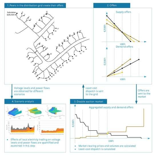
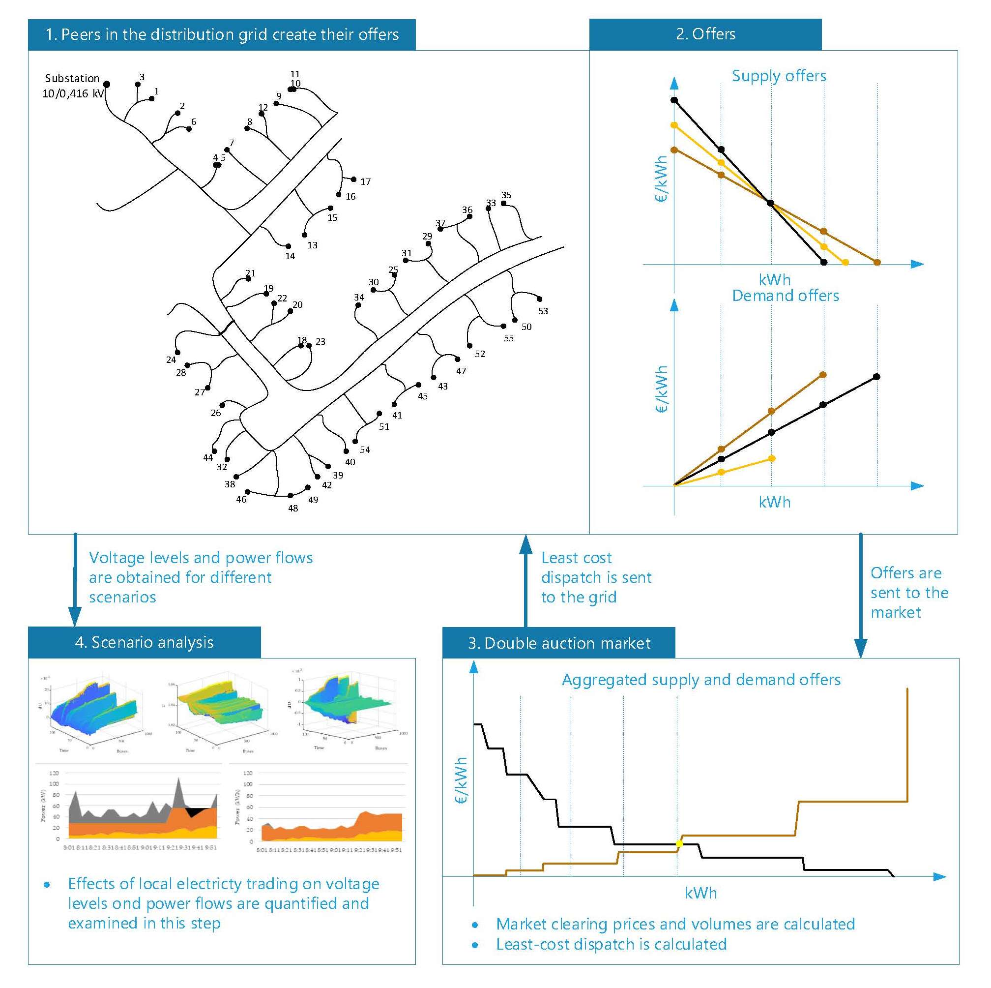
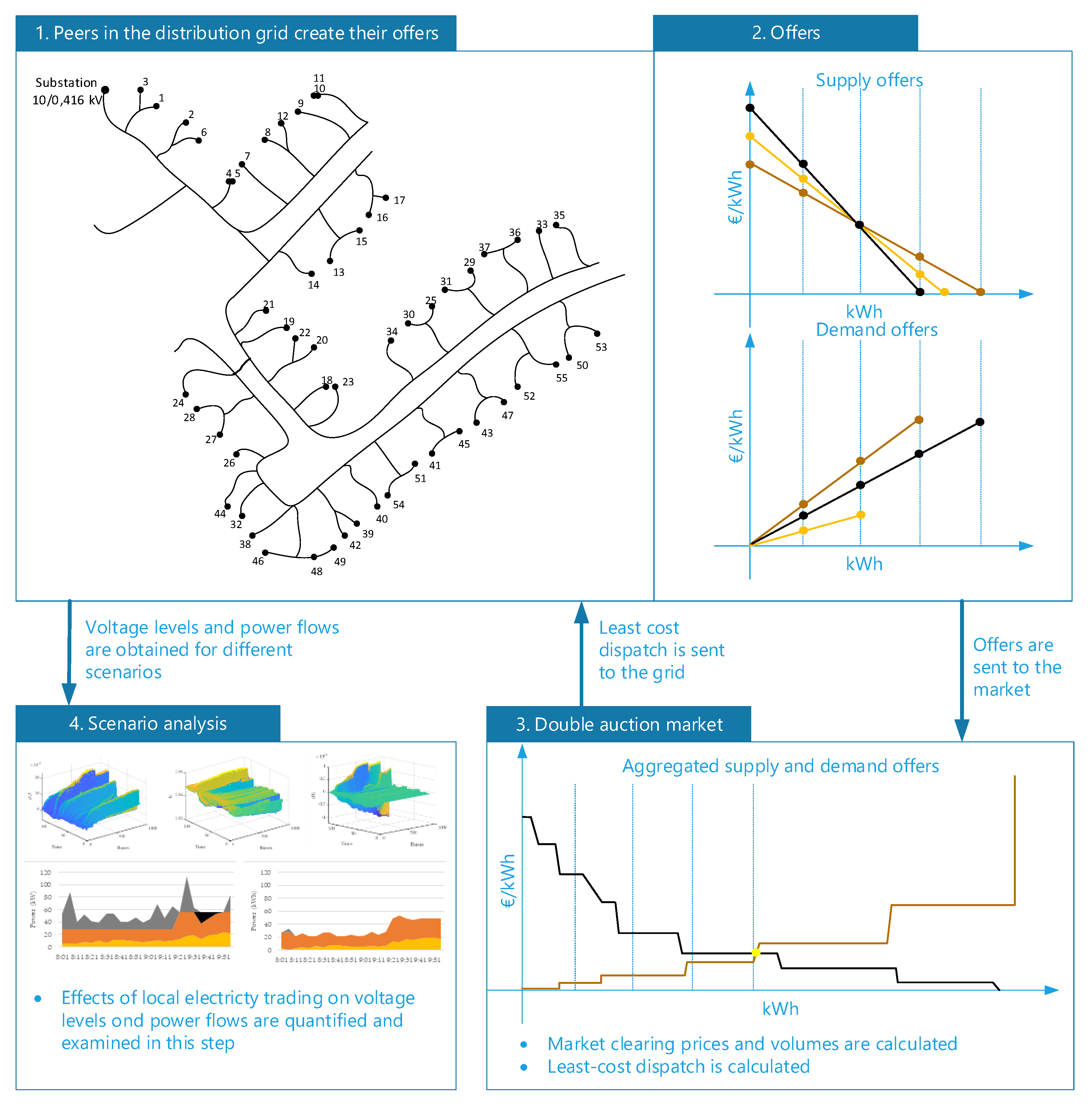
2. Method for Local Electricity Trading and Estimation of Its Impacts on the Grid

In order to investigate the issue of the voltage stability in the case of different LET strategies and offering curves, the centrally aggregated double auction LET algorithm was developed based on the EUPHEMIA [30] algorithm approach. The time horizon of the simulated market layer is 24 h, with 5 min resolution. From the developed algorithm, equilibrium prices and volumes (unit commitment of the peers) with a five-minute resolution is obtained. The dispatch of the committed peers is used as an input to the IEEE European LV Test Feeder [29] to analyze the power flows and voltage levels. The flowchart of the applied method is presented in the Figure A1 in the Appendix A. It is shown that in the first step, demand and supply offers are created by the peers in the distribution grid, based on their demand needs, demand elasticity, supply capacity, and supply offering prices. Afterward, all supply and demand offers are sent to the double-auction market, where offers are aggregated, and equilibrium volumes and prices are determined. Finally, the least-cost dispatch is sent to the IEEE European LV Test Feeder grid, where the effects of LET on power flows and voltage levels are studied.

The simulation of the IEEE European LV Test Feeder is conducted with one-second resolution using a five-minute dispatch from the previous step, resulting in the voltage profiles over 24 h time-horizon and in a resolution of one second. Scenario analysis is conducted for four cases of (supply and demand) offering curves of peers which simulate events from high to low electricity prices and high to low demand elasticity in the microgrid market. Also, the comparative analysis of the LET simulation results and the reference scenario simulation results on the IEEE European LV Test Feeder is provided. In the following subsections, the methods for the LET utilizing prosumer demand flexibility and different supply offering curves, as well as network model, are briefly explained.

2.1. Auction-Based Method for LET

The goal of the first stage of the simulation is to find a selection of offered supply and demand blocks that satisfy the energy balance requirement and maximize the global welfare defined as in Equation (1):

$$\max \left\{{\displaystyle \sum }_{t=1}^T{\displaystyle \sum }_{b=1}^B{\displaystyle \sum }_{i=1}^I(-ACCEP{T}_{s,t,b,i}·q_{s,t,b,i}·p_{s,t,b,i}+ACCEP{T}_{d,t,b,i}·q_{d,t,b,i}·p_{d,t,b,i})\right\}$$

(1)

The supply offers in Equation (1) have a negative sign. In this way, producer costs are minimized (which is equivalent to maximizing producer profit or surplus), and gross consumer surplus is maximized. Since demand is price-sensitive (elasticity > 0) in the assumed market, the goal function needs to include demand offers (called double–auction market). Otherwise, if demand is assumed to be completely insensitive to prices, the benefit received by the consumer is constant and does not need to be taken into consideration in the goal function. Under these conditions, the goal function would be represented by minimizing the total cost of producing energy. The goal function for global welfare maximization is subject to market and technical constraints that include:

-

energy balance constraints for each time period $t$, in time horizon made of $T$ periods, as listed in Equation (2):

$${\displaystyle \sum }_{b=1}^B{\displaystyle \sum }_{i=1}^{I}ACCEP{T}_{s,t,b,i}·q_{s,t,b,i}\ge {\displaystyle \sum }_{b=1}^B{\displaystyle \sum }_{i=1}^{I}ACCEP{T}_{d,t,b,i}·q_{d,t,b,i}$$

(2)

-

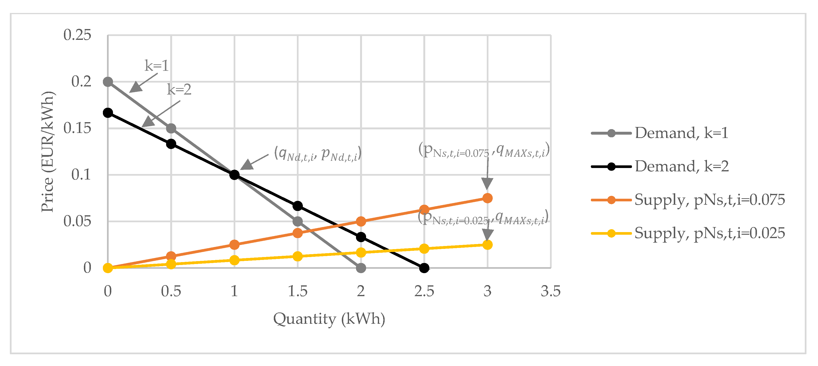
technical constraints of maximal supply and demand capacities for each peer $i$ in period $t$ ($q_{{MAX}_{s,t,i}}$ and $q_{{MAX}_{d,t,i}}$ respectively) have to be integrated into demand and supply offers, while individually can be written as in Equations (3) and (4):

$$0\le {\displaystyle \sum }_{b=1}^B{q}_{s,t,b,i}\le q_{{MAX}_{s,t,i}}$$

(3)

$$0\le {\displaystyle \sum }_{b=1}^B{q}_{d,t,b,i}\le q_{{MAX}_{d,t,i}}$$

(4)

In Equations (1)–(4) {s, d} is the index set of the offer types, and s means supply, d means demand. The $t$ is discrete time step over simulated time horizon $t\in \left\{1,2,\dots , T\right\}$. The $b$ is offer block, $b\in \left\{1,2,\dots , B\right\}$. The $i$ is the index of the peer, $i\in \left\{1,2,\dots , I\right\}$. $ACCEP{T}_{s,t,b,i}$ is the binary acceptance variable for supply offer of the peer $i$, in block $b$ and period $t$, $ACCEP{T}_{s,t,b,i}\in \left\{0,1\right\}$. $ACCEP{T}_{d,t,b,i}$ is the acceptance variable for demand offer of the peer $i$, in block $b$ and period $t$, $ACCEP{T}_{d,t,b,i}\in \left\{0,1\right\}$. The $q_{s,t,b,i}$ is the offered supply volume of the peer $i$, in block $b$ and in period $t$. The $q_{d,t,b,i}$ is offered demand volume of the peer $i$, in block $b$ and in period $t$. The $p_{s,t,b,i}$ is the offered supply price of the peer $i$, in block $b$ and in period $t.$ The $p_{d,t,b,i}$ is the offered demand price of the peer $i$, in block $b$ and in period $t$.

The final solution of the goal function (Equation (1)) finds the equilibrium volumes, but in some cases, there could be a mismatch between committed generation and demand (Equation (2)) due to the possible generation constraints and constraints in consumer consumption. The aim is to equalize as much as possible the generation and production, which means equilibrium price is approximated as a midpoint of marginal producer and marginal consumer prices (the MATLAB code that solves this issue is provided in the Supplementary Materials).

In order to simulate behavior of LET in the distribution network feeder, the centralized double auction mechanism such as EUPHEMIA is suitable. Here, the SCUC, which would internally include line limits as well as voltage and phase angle constraints as constraints in the auction method [31], is not implemented. The reason for this is due to the fact that we analyze bus voltages resulting from the anarchy behavior of different bidding approaches of the peers. This is done by analyzing power flows and voltage levels in a distribution grid in a case when SCUC and SCED calculations are not performed for observed time horizon and each trading period, respectively. Additional technical details on the EUPHEMIA algorithm is available in [30].

2.2. Method for Simulation of Effects of LET on LV Distribution Grid Power Flows and Voltage Levels

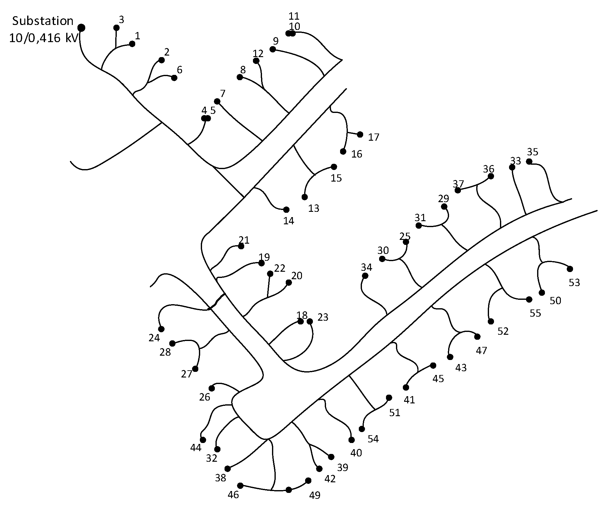
The dispatched supply and demand quantities of the peers from the first stage of the simulation framework are used in the second stage to simulate the effects on the voltage stability in the LV distribution network. As a reference network model for the simulation, the IEEE European LV Test Feeder [29,32] was selected. The IEEE European LV Test Feeder is a radial distribution feeder at the voltage level of 416 V (phase-to-phase) and a base frequency of 50 Hz, which is typical for the European low voltage distribution systems [32]. The application of the test feeder is suitable for the distribution research and planning, as it enables analysis of time-series rather than static power flow solutions. This is becoming increasingly important for analyzing dynamic behavior of different products and concepts on the distribution network, such as integration of DERs, Volt/VAr control, operation of BESS, etc. [32], as well as for application of simulations in various timeframes. Moreover, the feeder fits well with the topology of the island Krk distribution grid, where the LET will be implemented under the IMPACT project [8,33]. Therefore, the IEEE European LV Test Feeder is recognized as the most suitable for simulation and analysis of the effects of LET on voltage levels and power flows. The network topology of the test feeder is shown in Figure 1 [32,34,35].

3. Case Study

The case study assesses the impacts of different supply and demand offering strategies. Supply offer curves strategies reflect moments of high electricity prices and scarcity of supply in some scenarios and low electricity prices and oversupply in other scenarios. The demand offering curves reflect different flexibility and demand response abilities of the peers, as the demand curve elasticity is varied between the scenarios.

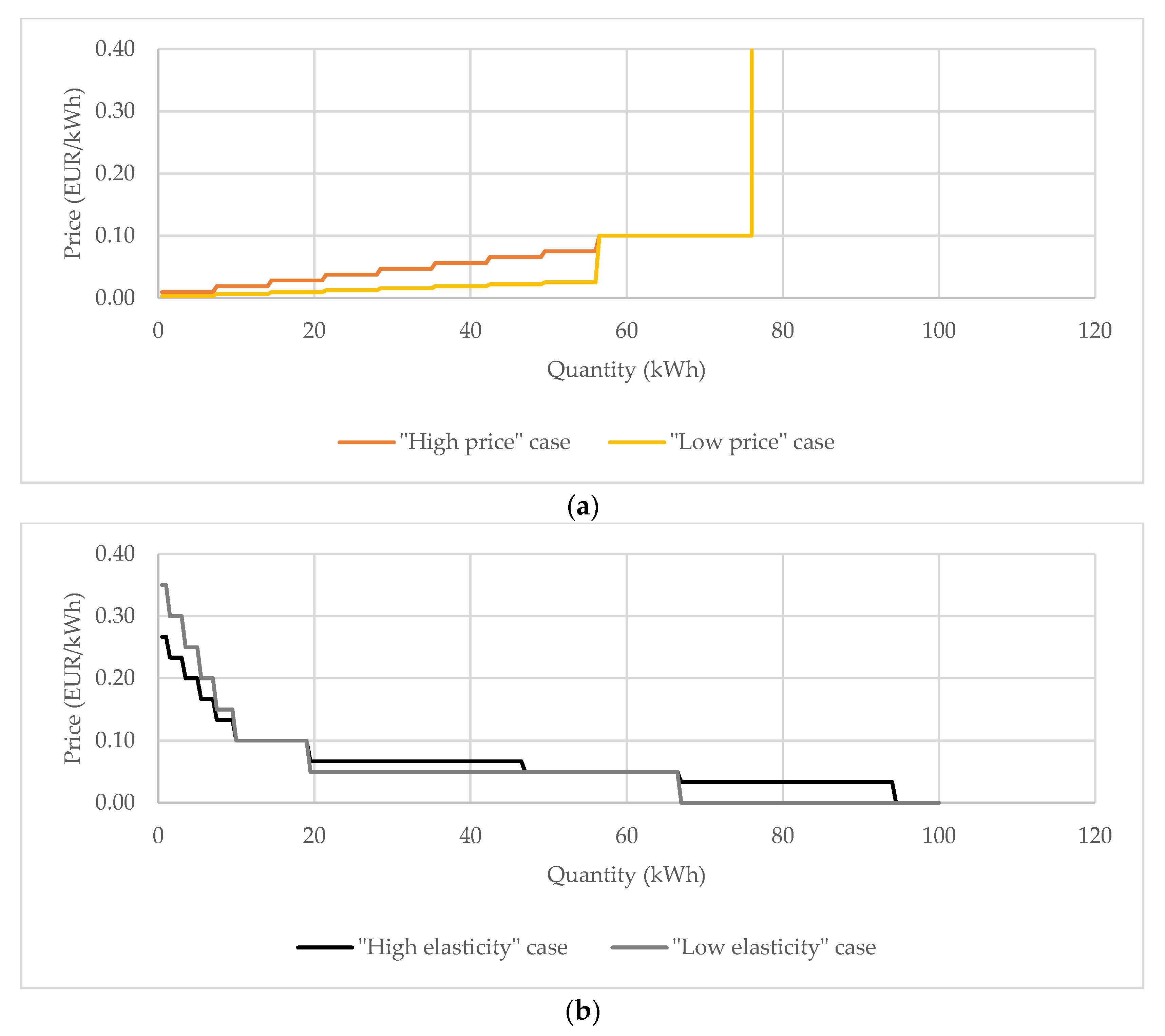
3.1. Scenarios and Input Data

The behavior of the production peers is analyzed for the two extreme behaviors: (1) when they practice higher markup, i.e., they aim to achieve additional revenue on top of actual cost and are ready to restrain from production and (2) when they bid with the lower offering prices, i.e., close to the short-run marginal costs (SRMC) and are expecting higher volumes of energy sold. The behavior of demand peers is varied based on the demand elasticity in two cases: (1) higher elasticity, where the application of demand response is assumed possible to a greater extent, and (2) lower elasticity, where the application of demand response is assumed possible to the lower extent. The demand in this microgrid is generally assumed inelastic in the area where local demand and supply curves intersect (absolute value of elasticity < 1), which is common in the electricity market [36,37] and this elasticity is increased and decreased to obtain the two demand elasticity scenarios on which price scenarios are tested.

Based on the variations of the behavior of the peers, the four scenarios are created (scenarios S1-S4). Moreover, the reference scenario (SREF) is assessed where the production is assumed maximal. It is a hypothetical case simulating the existence of feed-in tariffs for electricity production from renewable energy sources. Also, in this scenario demand is inelastic, as it represents the passive behavior of the peers as in traditional electricity LV distribution systems. The key differences of the analyzed scenarios and the used input data for individual peers are shown in

Table 1. Key differences of the analyzed scenarios and input data for individual peers, where “High” supply price is set at 0.075 EUR/kWh and “Low” supply price at 0.025 EUR/kWh.

Scenario	S1	S2	S3	S4	SREF
Maximal supply offering price	High	High	Low	Low	NA (feed-in-tariff)
Price elasticity of demand	Increased	Decreased	Increased	Decreased	Perfectly inelastic (passive demand)

.

In all cases, the nominal consumption patterns are taken from the IEEE European LV Test Feeder [29] and it is assumed that every fourth peer is equipped with the PV systems of the nominal capacity of 4 kW. The time-pattern of possible maximal production from the PV systems for the analyzed day was taken from [38] for 1 June. The minimum bidding blocks are assumed as 0.5 kW quantity. The creation of offering blocks for the peers is conducted in accordance with the Equations (5) and (6) for supply and demand, respectively, and is depicted in Figure 2.

$$p_{s,t,b,i}=\frac{p_{N_{s,t,i}}}{q_{{MAX}_{s,t,i}}}{q}_{s,t,b,i},\hspace{1em}where: 0\le q_{s,t,b,i}\le q_{{MAX}_{s,t,i}}$$

(5)

$$p_{d,t,b,i}=-\frac{2·p_{N_{d,t,i}}}{1+k}{q}_{d,t,b,i}+\frac{p_{N_{d,t,i}}·2·q_{{MAX}_{d,t,i}}}{1+k},\hspace{1em}where: 0\le q_{d,t,b,i}\le q_{{MAX}_{d,t,i}}$$

(6)

where $p_{N_{s,t,i}}$ is the nominal supply price (final price in the supply curve) of the peer $i$ in period $t$, $p_{N_{d,t,i}}$ is the nominal demand price of the peer $i$ in period $t$. It is assumed the same as the supply price from the utility grid, i.e., 0.100 EUR/kWh. Reference consumption $q_{N_{d,t,i}}$ of the peer $i$ in period $t$ (reference values are taken from the IEEE European LV Test Feeder) can be increased by the $k$ blocks where each block equals 0.5 kW, i.e., $q_{{MAX}_{d,t,i}}=$ $q_{{d,N}_{t,i}}+\frac{1+k}{2}$ (kW).

The applied approach for creating supply and demand offers allows transparent and tractable analysis using the nominal (final) supply prices $p_{N_{s,t,i}}$ and slopes of the demand curves around the nominal price $p_{N_{d,t,i}}$ (see Figure 2). The effects of varying nominal prices of the supply curve and slope around the nominal price of the demand curves are shown in Figure 2.

Moreover, in all scenarios, it is assumed that the supply price from the utility grid is fixed at 0.100 EUR/kWh, and the price of selling to the utility grid is fixed at 0.050 EUR/kWh. Also, for the sake of clarity in the presentation of the results and decreasing the simulation time, the time horizon of 120 min is analyzed in the case study. The analyzed timeframe is from 8 a.m. to 10 a.m. The chosen timeframe is the one when demand is available and production capacity from the installed PV systems of the peers is also available. The resolution of trading periods is 5 min, and the calculation of the voltages is presented in a one-minute resolution to ease the display of results of voltage level forms. Analysis of the longer timeframes is possible using the MATLAB code available in the Supplementary Materials.

Based on the input data listed above, the aggregated supply and demand curves are shown in Figure 3 for the time interval 9:35–9:40 a.m. In Figure 3a, the aggregated supply curves are shown for the “high price” and “low price” supply offers. In Figure 3b, the aggregated demand curves are shown for the “high elasticity” and “low elasticity” demand curves.

The aggregated merit order supply and demand offers are used to find the equilibrium prices and quantities in line with the methods presented in Section 2.1. In Figure 4, the found equilibrium prices and volumes are shown for the scenarios S1–S4, for the same time interval 9:35–9:40 a.m. The effects of different maximal supply offering prices and elasticities of demand are visible in the illustrative scenarios shown in Figure 4. In the S1 scenario, with “high prices” and “increased elasticity”, the found equilibrium price is the highest due to the impact of offers with high prices. In the S2 scenario, the effect of lower elasticity of the demand led to lower volumes and prices, meaning peers sold less energy. The S3 and S4 scenarios demonstrated the market-clearing under the assumption of “low prices”, and “increased elasticity” and “decreased elasticity”, respectively. Those assumptions led to the lower market-clearing prices and higher traded volumes.

Interestingly, due to the composition of the offering curves, the intersection point is the same in S3 and S4 scenarios. Also, it is evident that the effects of “low prices” in supply offers had a bigger impact compared to the changes in elasticity, which is due to the fact that changes in elasticity of electricity demand are relatively less intense compared to the changes in supply offer prices.

On those price and demand scenarios, the voltage stability is assessed in the second stage of the simulation for all the periods in the assessed time horizon. The simulation was conducted in MATLAB software environment [35].

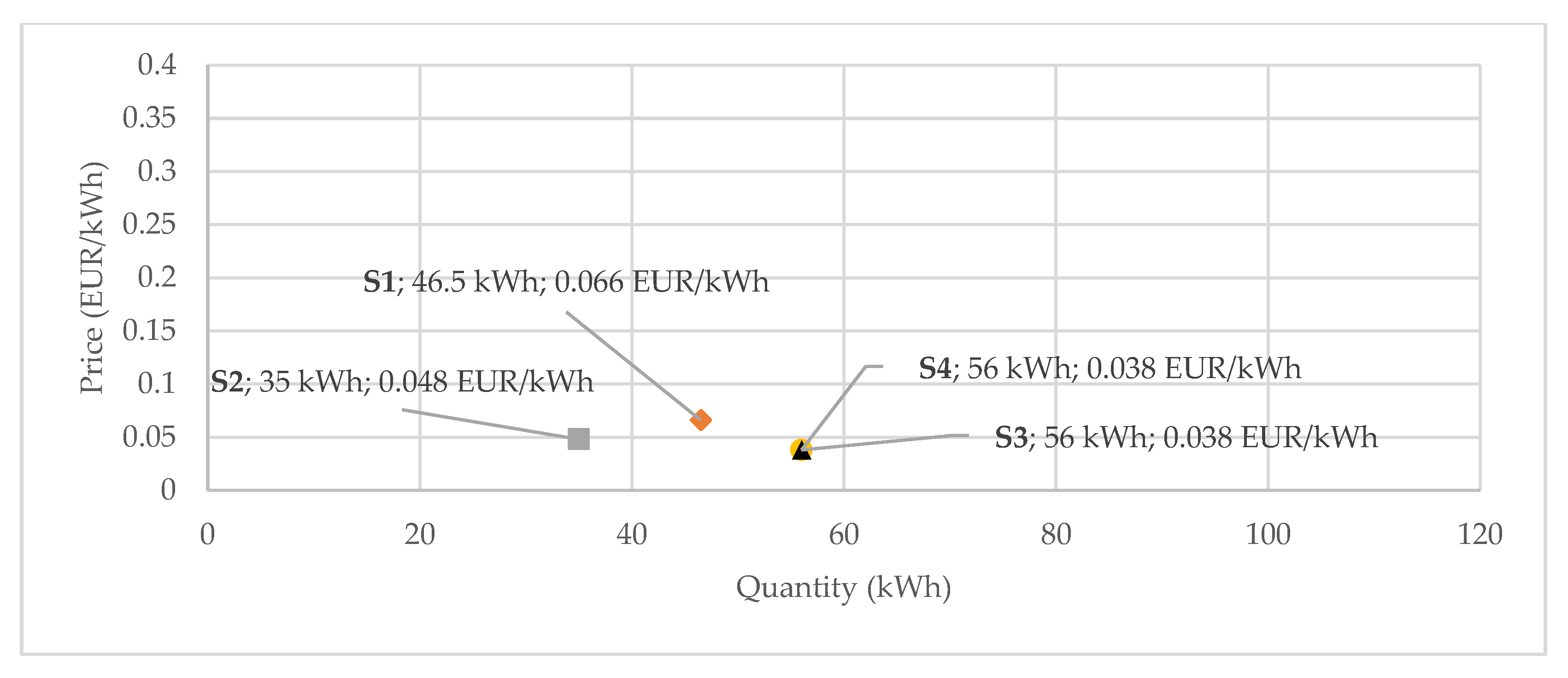
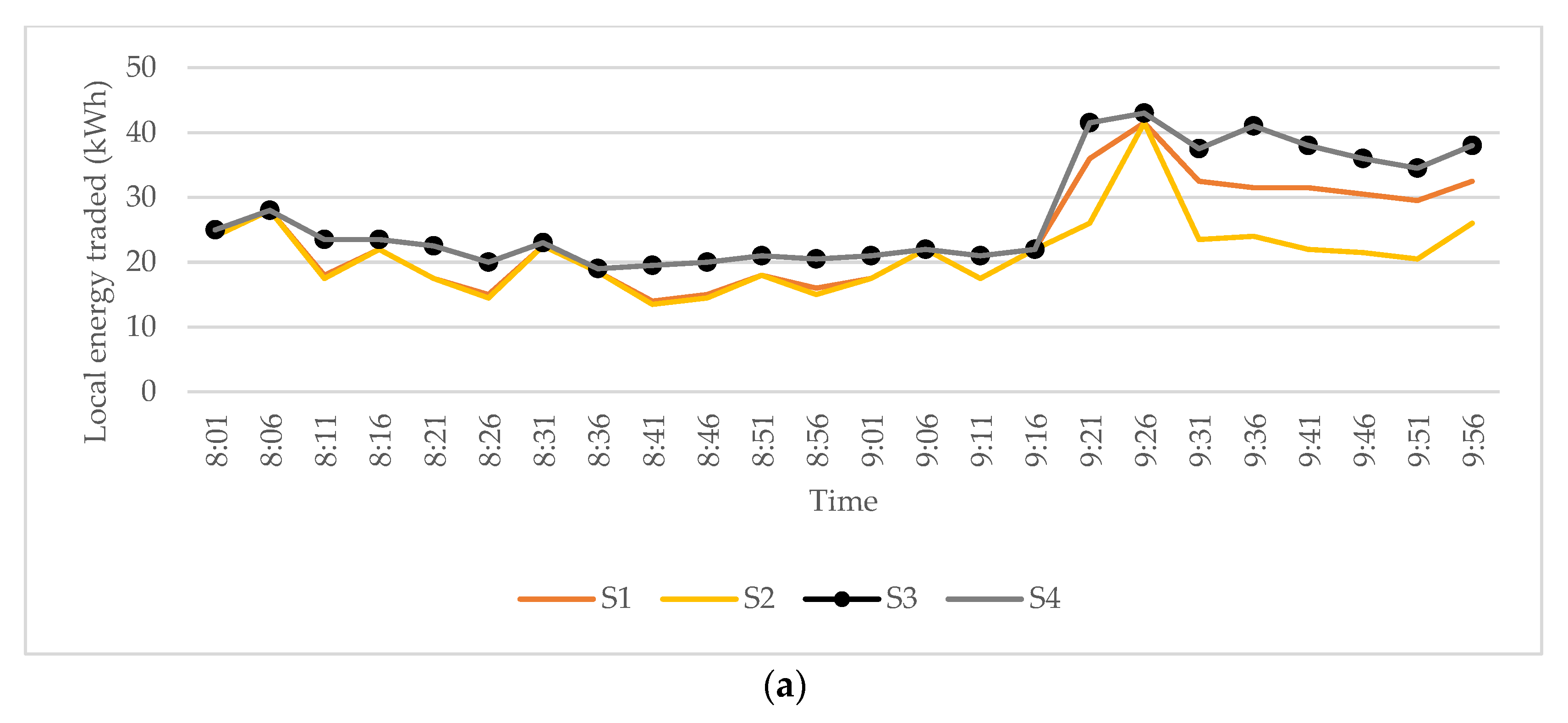
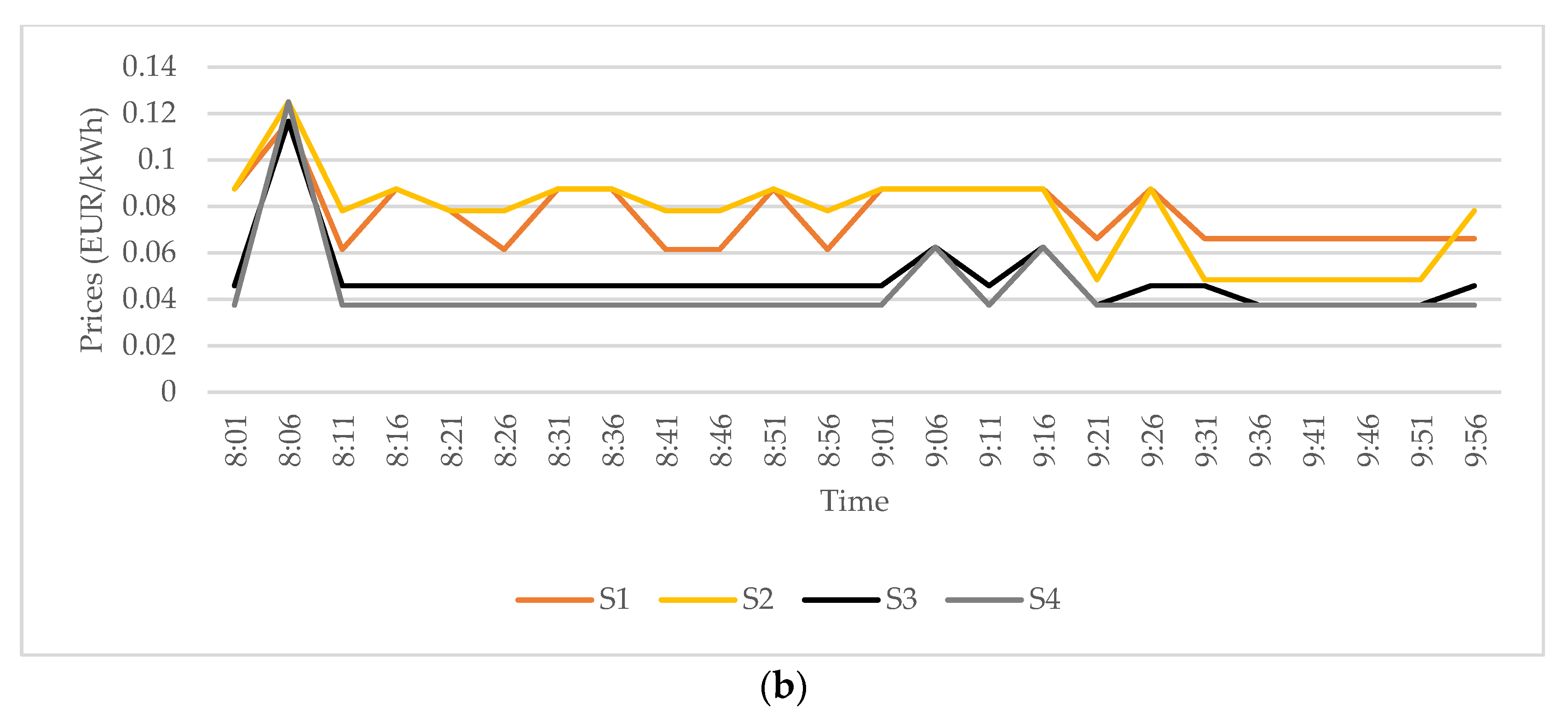
3.2. Outputs of the First Stage of the Simulation: Equilibrium Quantities and Prices

As elaborated in the previous section, the outputs of the first stage of the LET are the equilibrium prices, volumes, and least-cost dispatch calculation. The calculated dispatch is input for the second stage, i.e., analysis of the effects on voltage levels in the IEEE European LV Test Feeder. Due to the number of 55 peers, only the aggregated values are displayed in Figure 5. In Figure 5a, the equilibrium volumes are shown. In Figure 5b, the equilibrium prices are shown in the analyzed scenarios. Similarly to the analyzed one period in the previous subsection, the effects of different maximal supply offering prices and demand elasticities are here visible in a longer time horizon.

In the S2 scenario (Figure 5a), with “high prices” and “decreased elasticity”, the found equilibrium volumes are the lowest due to the fact that in the analyzed scenarios decrease of elasticity increases the slope of the demand curve, and since the aggregated nominal demand offer prices are higher than the aggregated supply offer prices for the aggregated nominal demand quantity, the decrease of the slope of demand offer curve decreases the equilibrium quantities. The effects on equilibrium prices (Figure 5b) for the analyzed scenarios are not always consistent (comparison of equilibrium prices for the scenarios S1 and S2 in the time period 8:00–9:15 a.m.), which is due to the fact the equilibrium prices are approximated as a midpoint of marginal producer and marginal consumer prices, in each period. That midpoint can be misleading n a case of a relatively small number of peers, and the equilibrium price can be determined more precisely with additional sub-problem, such as in EUPHEMIA algorithm [30]. However, for this research, it is out of the scope, as the equilibrium volumes are essential for analyzing the power flow and voltages. The scenarios S3 and S4 demonstrated the market-clearing under the assumption of “low prices”, and “increased elasticity” and “decreased elasticity”, respectively. Those assumptions led to the lower market-clearing prices and higher traded volumes. In the S4 scenario, the traded volumes correspond to the ones in scenario S3, but due to the lower elasticity of the demand curve, the equilibrium prices are lower on average.

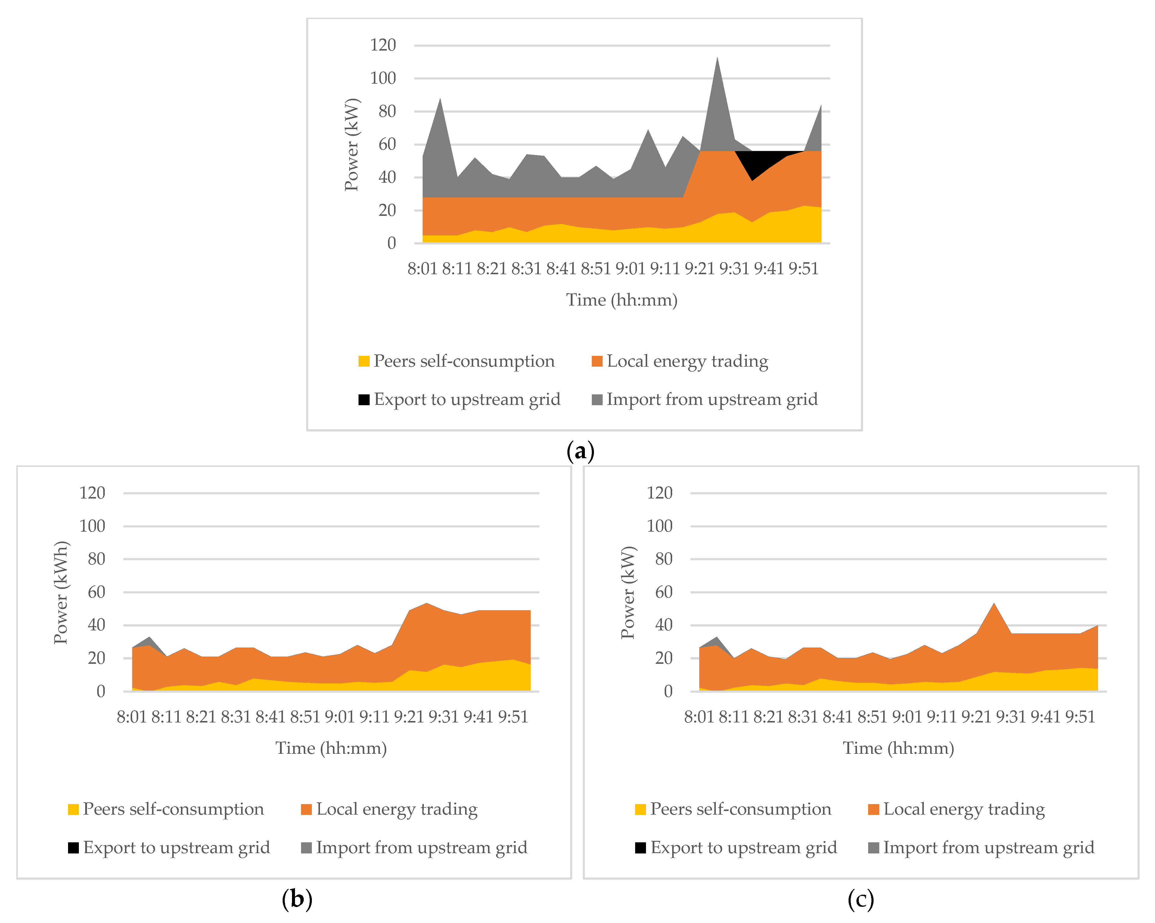
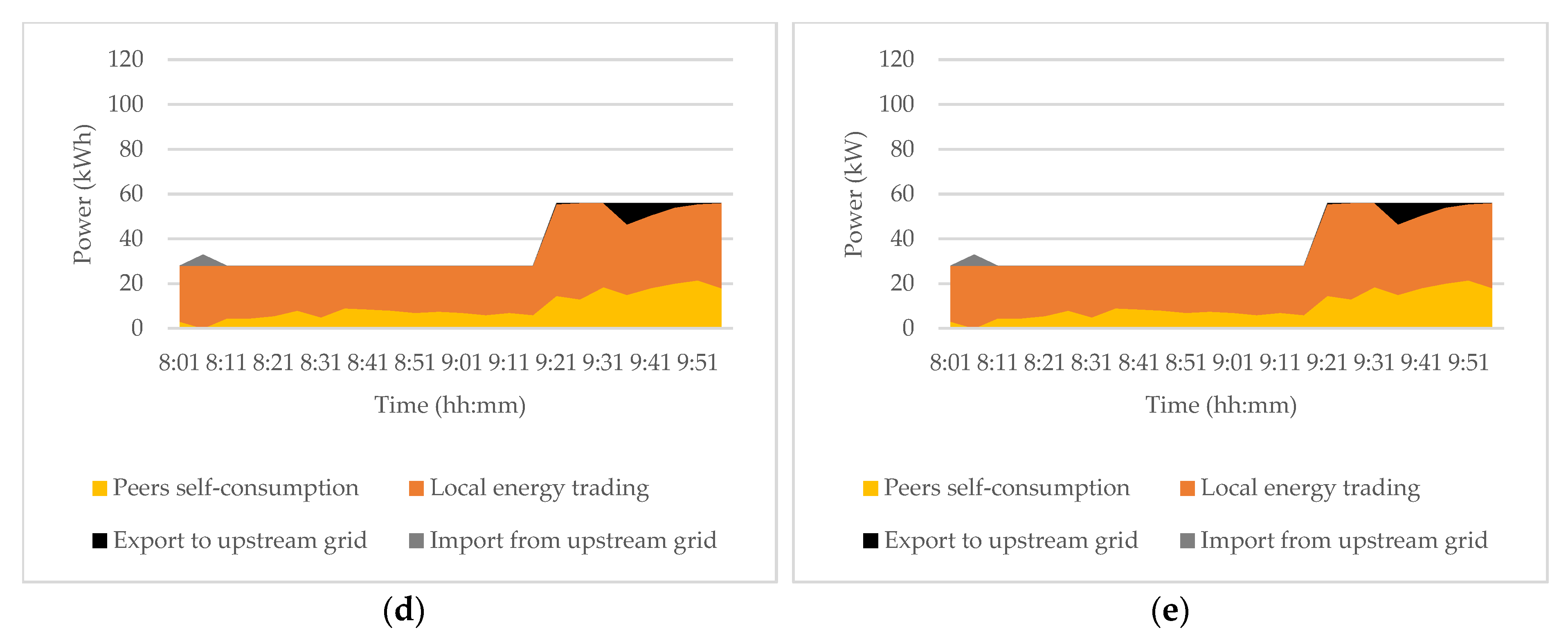
3.3. Results: Power Flows

The effects of trading and dispatched demand and supply quantities on microgrid energy balance for the observed period from 8:00 a.m. until 10:00 a.m. across the modelled scenarios are numerically shown in

Table 2. Energy balance (kWh) in the microgrid for the analyzed scenarios in the observed time horizon (from 8:00 a.m. until 10:00 a.m.).

Item	SREF	S1	S2	S3	S4
Total microgrid consumption	1321	783.5	687	883	883
Total microgrid production	896	778.5	682	896	896
Peers self-consumption	282	205.5	172.5	235	235
Local electricity trading	583	573	509.5	643	643
Import from upstream grid	456	5	5	5	5
Export to upstream grid	−31	0	0	−18	−18

and graphically in Figure 6. The energy balance is divided on the: (1) Peers self-consumption, which is the energy produced by the PV systems owned by the prosumers and consumed immediately at their locations, (2) Local energy trading in the observed distribution grid, which is the energy produced by the PV systems owned by the prosumers and not consumed by themselves but traded with the other peers in the local distribution grid, (3) Export to the upstream grid, which is the surplus energy exported out of the observed distribution grid, and (4) Import from upstream grid, which is the energy imported to the observed distribution grid in periods when local demand is higher than local supply.

It can be observed that in the scenario SREF (Figure 6a), the total consumption in the microgrid is at the nominal values and highest. Electricity production is also maximal, but with given demand and supply capacity ratio, the demand is higher for most of the time. Consequently, a significant share of energy consumed (34.5%) is imported from the upstream network in the SREF scenario (Table 2). In comparison, in the scenarios with implemented LET, where demand elasticity is defined by offer curves, a decrease of energy consumption and avoidance of extreme market prices is possible as elasticity enables consumers to buy less when the prices are higher (Figure 3 and Figure 4). In the S1 scenario, the LET with high offer prices and increased demand elasticity led to the decrease in total energy consumption by 40.7% and decrease in the energy production by 13.1% compared to the SREF scenario. Those effects combined led to the decrease in the imports from the upstream network from 34.5% to 0.6%. Also, the export to the upstream grid does not occur. In the S2 scenario, the decreased demand elasticity led to the decrease in energy consumption and decrease in locally traded electricity. Decrease of supply offering prices in scenarios S3 and S4 led to the increase of energy consumption and locally traded eletricity in the local distribution grid.

Due to the modeled demand elasticity, the social welfare maximization was found in conditions when the local production is maximal, and demand is adjusted to the supply levels. Moreover, the exports to the grid proved justified in those scenarios. The scenarios S3 and S4 are equal in terms of energy balance as the decrease of demand elasticity in the S2 scenario didn’t change the equilibrium quantities for the given input parameters.

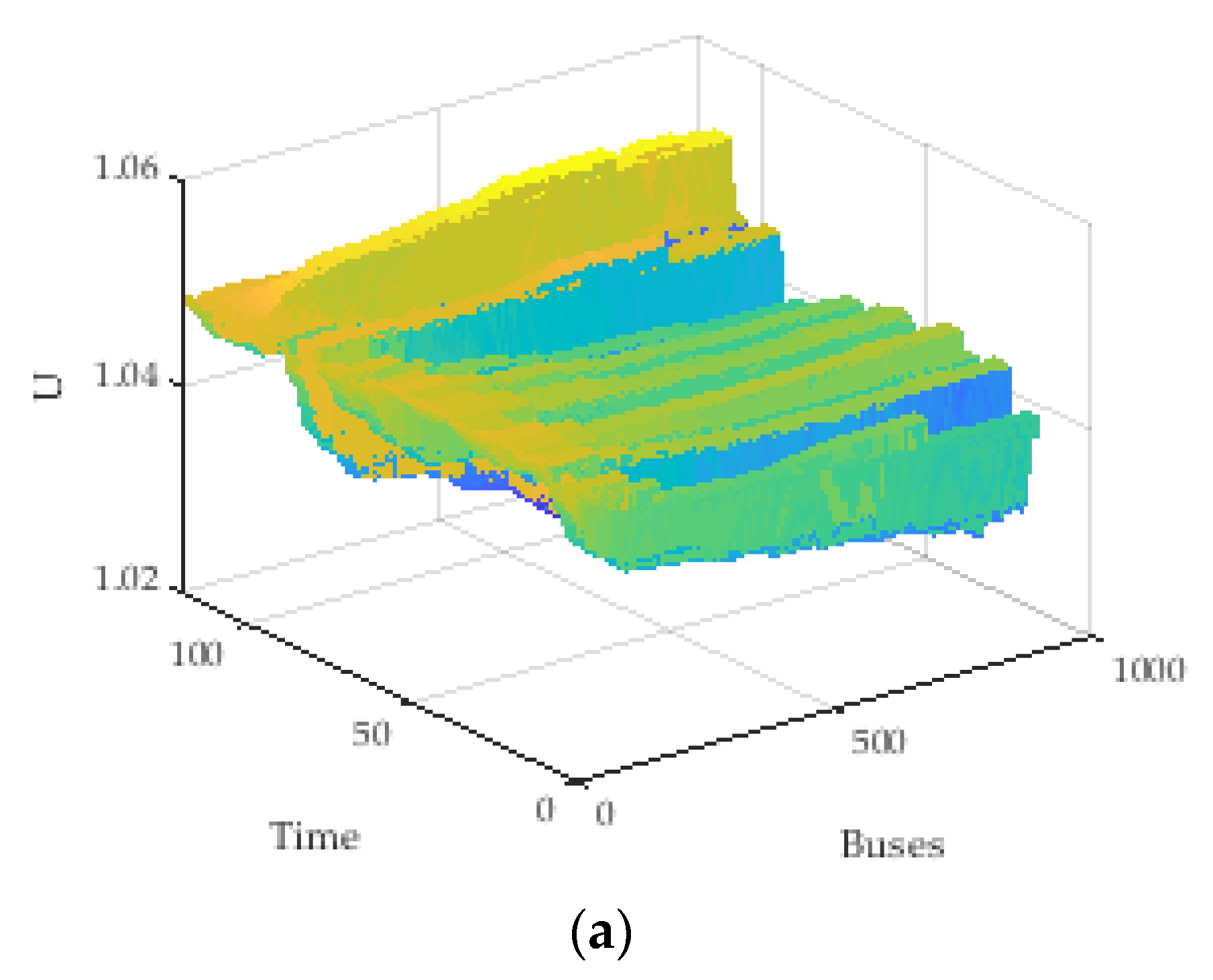
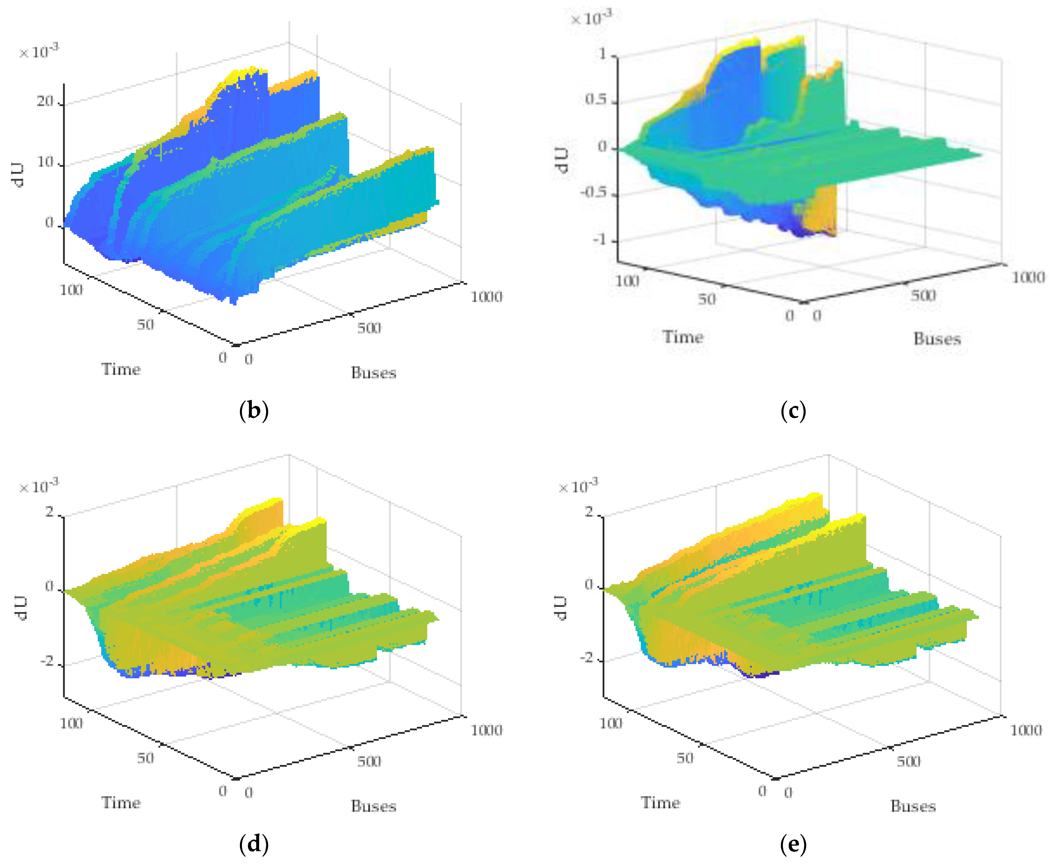
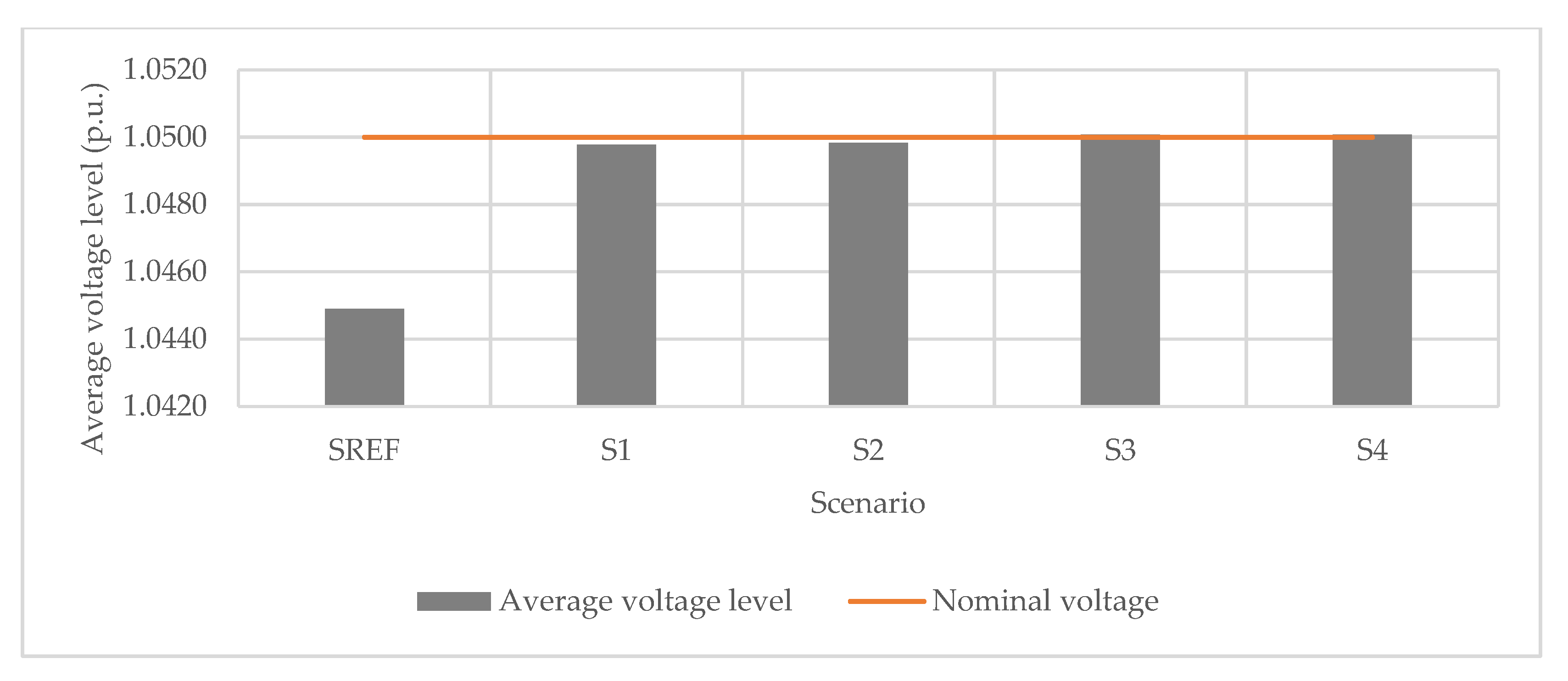
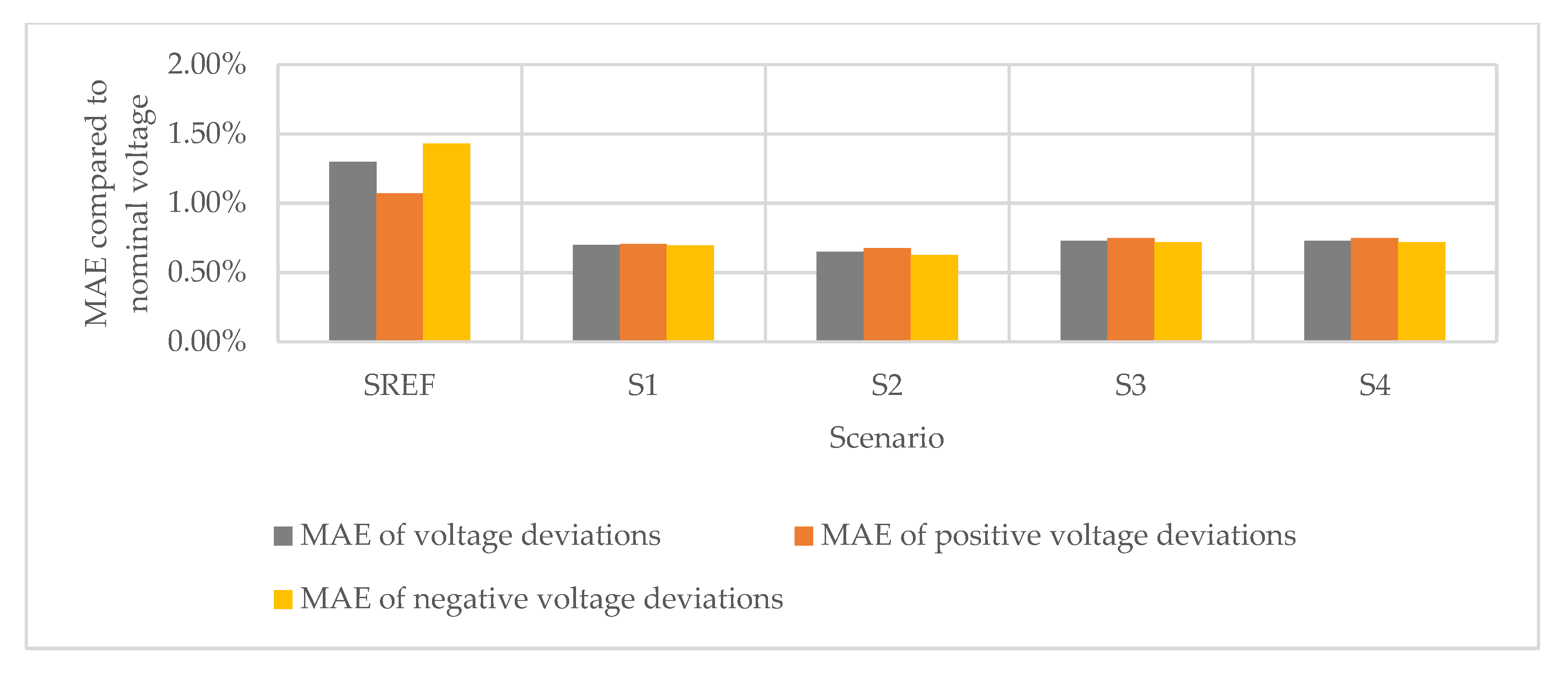
3.4. Results: Voltage Levels

Based on the outputs of the first stage of the simulation and calculated least-cost dispatch, the impacts of the dispatch on the voltage levels in the IEEE European LV test feeder are studied. In Figure 7, voltage (U) and voltage differences (dU) over time (minutes) for different busses are shown. Due to a large amount of data (voltages for 906 buses × 7.200 s × 3 phases × 5 scenarios), the chosen data is shown in 3D graphs and the voltages are displayed in a one-minute resolution. For a further overview of the results, the reader is advised to use the electronically available data and MATLAB files available in the Supplementary Materials, where detailed voltage results are available in an interactive form. In Figure 7a, voltage levels for 906 buses over 120 min for the reference scenario (SREF) are shown. The results presented in Figure 7b–e show the voltage differences between S1 and SREF; S1 and S2; S1 and S3; and S2 and S3 scenarios respectively.

Moreover, the average voltage levels and differences from the nominal voltage across the analyzed scenarios are summarized in

Table 3. Average voltage levels and difference of the average voltage level from the nominal in all scenarios.

Scenario	SREF	S1	S2	S3	S4
Average voltage level	1.04490	1.04977	1.04983	1.05008	1.05008
Average voltage level difference from the nominal	−0.486%	−0.022%	−0.016%	0.007%	0.007%

and shown in Figure 8. As visible in Figure 7, due to the fact that the tap changer ratio is set to 1.05 at the secondary side of the transformer, the voltage level at the bus 1 is 1.05 p.u. in all scenarios. In the SREF scenario (Figure 7a), it can be observed that the voltage levels are within the boundaries prescribed by the norms for the LV distribution grid (±10% from nominal voltage) [39]. Also, the voltage drop towards the end of the feeder can be observed, particularly at the buses where no distributed generation is present, which is a usual phenomenon in the distribution grid [40]. On average, the voltages are 0.486% below the nominal voltage (Table 3 and Figure 8). The comparison of the voltages in scenarios S1 and S2 (Figure 7a) shows that, on average, voltages in the S1 scenario are higher by 0.46% (Table 3) compared to the SREF scenario. This can be explained by the decrease of energy consumption and minimization of the imports from the upstream grid (Table 2 and Figure 6b) due to the active participation of peers in the LET and application of demand response, due to the high equilibrium prices. The consequent reduction of power flows from the transformer substation to the ends of the distribution grid leads to a decrease of currents from the upstream grid to the users in the microgrid and decreases the voltage drop, i.e., raises the voltage levels [40,41]. In the S2 scenario (Figure 7c, Table 3, and Figure 8), it can be observed that, on average, voltage levels are further slightly increased compared to the S1 scenario. That can be explained due to the fact that the decrease of demand elasticity in this scenario leads to the decrease of equilibrium volumes, decrease of energy consumption and decrease of locally traded electricity (Table 2 and Figure 6c), which in turn causes lower power flows from the upstream grid and decreases voltages drops, i.e., increases voltage levels. In the S3 scenario (Figure 7d), on average, voltages are higher compared to the S1 scenario (Figure 7c, Table 3, and Figure 8). This is due to the fact that in the S3 scenario equilibrium volumes of locally traded electricity are increased due to the lower offer prices. That leads to an increase of exports to the upstream network and to an increase of local power flows, due to increased distributed generation and demand balanced locally in the distribution grid (Table 2 and Figure 6d). Those power flows resulted in lower voltage drops [40], i.e., additionally increased voltage levels in the S3 scenario compared to the S2 scenario. The comparison of the scenarios S2 and S3 (Figure 7e), shows similar results as the comparison of the scenarios S1 and S3, i.e., the voltages in the S3 scenario are increased (Table 3 and Figure 8). It is due to the fact that the low offering prices increase energy consumption, production and the locally traded electricity (Table 2 and Figure 6d). In this case, those impacts are more significant than the impacts of the increased elasticity, which is causing the opposite effects (Table 2 and Figure 6e). From the Table 3 and Figure 8, it is also visible that the average voltage levels in the scenarios with the implemented LET are closer to the nominal voltage (0.006% below nominal, on average), compared to the SREF scenario (0.486% below nominal), meaning implementation of LET in distribution grid can contribute to decreasing voltage drops and stabilizing voltage levels.

Moreover, differences between voltage deviations in all scenarios compared to the nominal voltage are quantified using the mean absolute error (MAE). That way, additional comparisons can be made and provide interesting insights into the effects of offer prices and demand elasticity on voltage levels and voltage deviations. In

Table 4. MAE between grid voltage and nominal voltage (for all deviations, positive deviations, and negative deviations) over all periods, busses, and phases. For the clarity of the results, MAE is divided by the nominal voltage and expressed as a percentage.

Scenario	SREF	S1	S2	S3	S4
MAE (all voltage deviations) (%)	1.300%	0.700%	0.650%	0.730%	0.730%
MAE (positive voltage deviations) (%)	1.072%	0.707%	0.676%	0.751%	0.751%
MAE (negative voltage deviations) (%)	1.432%	0.697%	0.626%	0.718%	0.718%

and Figure 9, deviations from the nominal voltage are quantified using MAE for all voltage deviations (dU), positive voltage deviations (dU⁺) and negative voltage deviations (dU⁻).

From Table 4 and Figure 9, it can be observed that in the SREF scenario, MEA for all voltage deviations equals to 1.30% of the nominal voltage, and the dominant are negative voltage deviations (1.43% for the negative compared to the 1.07% for the positive deviations). The sum of the deviations led to the decrease of the voltage levels from the nominal by −0.486%, as seen in Table 3 and Figure 8. In all scenarios that include simulation of the active LET (scenarios S1–S4), MAE is nearly halved for all voltage deviations (ranges from 0.65% to 0.73%). In the S1 scenario (high supply prices, increased demand elasticity) the MAE of all voltage deviations equals 0.70%, with the domination higher impact of positive voltage deviations (0.71%) compared to the MAE of negative voltage deviations (0.70%). However, even though the MAE of positive voltage deviations is higher, the average voltage level dropped by 0.022% compared to the nominal, which means that there is a larger number of the negative voltage deviations. The effects of the decreased demand elasticity in the S2 scenario led to a decrease in total energy consumption and decrease in volumes of locally traded electricity (Figure 6 and Table 2). That, in turn, led to the decrease of voltage deviations (all, positive, and negative) (Table 4, Figure 9) and to a slight rise of the average voltage level (Table 3, Figure 8), in comparison with the S1 scenario. The decrease of supply offering prices in scenarios S3 and S4 led to an increase in the total energy consumption, production, and increase in volumes of locally traded electricity (Figure 6 and Table 2). Moreover, it led to the exports to the upstream grid, which in turn led to the upstream power flows, increase of average voltage level (Table 3, Figure 8), and to the increase of voltage deviations, especially positive voltage deviations (Table 4, Figure 9), in comparison with the scenarios S1 and S2. Finally, it can be seen that the MAE of voltage deviations in the scenarios with the active LET are, on average, 54% lower than in the SREF scenario.

4. Discussion

The paper proposes the method for simulation and analysis of the effects of different elasticities and prices in offering curves of the peers participating in the LET, on power flows and voltage levels in the distribution grid. The proposed LET is based on a centrally aggregated double-auction trading mechanism and applied in the IEEE European LV Distribution Grid Test Feeder. The paper contributes with the assessment and exploration of implications of implementing LEMs in distribution grid with a significant RES capacity and active participation of prosumers through demand response. Also, it is investigated if LEMs can be operated without time-consuming SCUC calculations for observed time horizons and without SCED calculations for each trading period. The analysis includes implications on the power flows and voltage stability on the local distribution grid.

The results point out at several valuable insights. LET can significantly contribute to the local supply-demand balancing and thus decrease the imports from the upstream grid. In a LEM organized in an auction-based manner, the participants’ strategies for demand and supply offering curves have significant impact on market-clearing prices and quantities, i.e., local electricity consumption and production, and thus affect the initiated power flows and voltage levels. At the same time, LEM market-clearing prices and quantities significantly depend on the organization of the LEM and integration with the rest of the electricity market, particulary on the prices and quantities of electricity that can be sold to, or bought from the upstream grid. Also, the scenario analysis has shown that, within the given boundary conditions, LET can be operated without SCUC and SCED calculations for each trading period. The analysis of the effects of supply and demand offering strategies showed that the low supply offering prices contribute to the rise in the local electricity consumption and production, rise in the volumes of locally traded electricity and as well potentially higher exports to the upstream grid, consequently increasing the voltage levels. On the contrary, high supply offering prices have opposite impacts. The effects of demand elasticity changes depend on the shape of the demand curves and relation with the supply curves, so the effects are not unambiguous, as the increase of demand elasticity can lead to the effects similar to the ones caused by the low supply offering prices but not necessarily. In the observed scenarios, the decrease of demand elasticity led to the decrease of equilibrium prices and volumes, while the decrease of supply offering prices led to the increase of local energy consumption and volumes traded. The effects on average voltage levels in considered scenarios primarily depended on the power flows from/to the upstream grid, as the improvement of local electricity supply-demand balancing (behind the substation) led to the minimization of voltage drops and to the increase in voltage levels. Moreover, that way voltage deviations were also decreased.

Those effects can have important implications for designing the LEMs and associated market and control mechanisms. Also, insights could have impacts on the operation of distribution systems where LEMs are implemented, as DSOs could reduce LV levels at the secondary side of distribution transformers in order to address the effects of LETs on voltage levels.

Future work and research include the exploration of the voltage and frequency response in the cases when LET is implemented in microgrids that can operate in the island mode. Further, in the IMPACT project [33], a laboratory setup for testing LET concepts in small-scale microgrids, and real-life testing in a community microgrid is foreseen. Moreover, since the used model for LET is based on the EUPHEMIA algorithm [30], it means that electricity trading between microgrids can be organized in an analogy to the market coupling between the zones of the wholesale markets, where microgrids would serve as zones in the wholesale markets. Thereby, the cross-border lines of the wholesale markets can be represented by substations between neighboring microgrids, and substation rated power would serve as a total transfer capacity (TTC). For the calculation of the net transfer capacity (NTC), TTC has to be reduced by the transmission reliability margin (TRM) to cover for the forecast uncertainties and probabilistic real-time events [42]. Further, available transfer capacity (ATC) could be calculated as NTC reduced by the notified transmission flows (NTF), which covers for the already reserved contract sizes (for example, day-ahead or hour-ahead contracts between microgrid participants). Consequently, the idea is that the final ATC would serve as a transfer capacity that remains available for further commercial LET activity and is used in the market coupling algorithm [30,42]. That way, implicit cross-microgrid capacity allocation mechanism and trading could be implemented in the code in the future.

References

1. Kampman, B.; Blommerde, J.; Afman, M. The Potential of Energy Citizens in the European Union; CE Delft: Delft, The Netherlands, 2016. [Google Scholar]
2. Fleer, J.; Zurmühlen, S.; Meyer, J.; Badeda, J.; Stenzel, P.; Hake, J.-F.; Sauer, U.S. Techno-economic evaluation of battery energy storage systems on the primary control reserve market under consideration of price trends and bidding strategies. J. Energy Storage 2018, 17, 345–356. [Google Scholar] [CrossRef]
3. Güngör, V.C.; Sahin, D.; Kocak, T.; Ergüt, S.; Buccella, C.; Cecati, C.; Hancke, G.P. Smart grid technologies: Communication technologies and standards. IEEE Trans. Ind. Inform. 2011, 7, 529–539. [Google Scholar] [CrossRef] [Green Version]
4. Burke, M.J.; Stephens, J.C. Energy democracy: Goals and policy instruments for sociotechnical transitions. Energy Res. Soc. Sci. 2017, 33, 35–48. [Google Scholar] [CrossRef]
5. Khorasany, M.; Mishra, Y.; Ledwich, G. Market framework for local energy trading: A review of potential designs and market clearing approaches. IET Gener. Transm. Distrib. 2018, 12, 5899–5908. [Google Scholar] [CrossRef] [Green Version]
6. Parag, Y.; Sovacool, B.K. Electricity market design for the prosumer era. Nat. Energy 2016, 1, 16032. [Google Scholar] [CrossRef]
7. Morstyn, T.; Farrrel, N.; Darby, S.J.; McCulloch, M.D. Using peer-to-peer energy-trading platforms to incentivize prosumers to form federated power plants. Nat. Energy 2018, 3, 94–101. [Google Scholar] [CrossRef]
8. Ilak, P.; Rajšl, I.; Herenčić, L.; Zmijarević, Z.; Krajcar, S. Decentralized electricity trading in the microgrid: Implementation of decentralized peer-to-peer concept for electricity trading (P2PCET). In Proceedings of the Mediterranean Conference on Power Generation, Transmission, Distribution and Energy Conversion (MEDPOWER 2018), Dubrovnik, Croatia, 12–15 November 2018. [Google Scholar] [CrossRef]
9. Mengelkamp, E.; Gärttner, J.; Rock, K.; Kessler, S.; Orsini, L.; Weinhardt, C. Designing microgrid energy markets: A case study: The Brooklyn Microgrid. Appl. Energy 2018, 210, 870–880. [Google Scholar] [CrossRef]
10. Zhang, C.; Wu, J.; Zhou, Y.; Cheng, M.; Long, C. Peer-to-Peer energy trading in a Microgrid. Appl. Energy 2018, 220, 1–12. [Google Scholar] [CrossRef]
11. Herenčić, L.; Ilak, P.; Rajšl, I.; Zmijarević, Z.; Cvitanović, M.; Delimar, M.; Pećanac, B. Overview of the main challenges and threats for implementation of the advanced concept for decentralized trading in microgrids. In Proceedings of the IEEE EUROCON 2019-18th International Conference on Smart Technologies, Novi Sad, Serbia, 1–4 July 2019. [Google Scholar] [CrossRef]
12. Hirsch, A.; Parag, Y.; Guerrero, J. Microgrids: A review of technologies, key drivers, and outstanding issues. Renew. Sustain. Energy Rev. 2018, 90, 402–411. [Google Scholar] [CrossRef]
13. Morstyn, T.; McCulloch, M. Multi-class energy management for peer-to-peer energy trading driven by prosumer preferences. IEEE Trans. Power Syst. 2019, 34, 4005–4014. [Google Scholar] [CrossRef]
14. Shuai, Z.; Sun, Y.; Shen, Z.J.; Tian, W.; Tu, C.; Li, Y.; Yin, X. Microgrid stability: Classification and a review. Renew. Sustain. Energy Rev. 2016, 58, 167–179. [Google Scholar] [CrossRef]
15. Đaković, J.; Ilak, P.; Baškarad, T.; Krpan, M.; Kuzle, I. Effectiveness of wind turbine fast frequency response control on electrically distanced active power disturbance mitigation. In Proceedings of the Mediterranean Conference on Power Generation, Transmission, Distribution and Energy Conversion (MEDPOWER 2018), Dubrovnik, Croatia, 12–15 November 2018. [Google Scholar] [CrossRef]
16. Levron, Y.; Guerrero, J.M.; Beck, Y. Optimal power flow in microgrids with energy storage. IEEE Trans. Power Syst. 2013, 3, 3226–3234. [Google Scholar] [CrossRef] [Green Version]
17. Lin, J.; Magnago, F.H.; Foruzan, E.; Albarracín-Sánchez, R. Chapter 8—Market design issues of distributed generation. In Distributed Generation Systems; Gharehpetian, G.B., Agah, S.M.M., Eds.; Butterworth-Heinemann: Oxford, UK, 2017; pp. 369–413. [Google Scholar] [CrossRef]
18. Feng, X.; Shekhar, A.; Yang, F.; Hebner, R.E.; Bauer, P. Comparison of hierarchical control and distributed control for microgrid. Electr. Power Compon. Syst. 2017, 10, 1043–1056. [Google Scholar] [CrossRef]
19. Netztechnik/Netzbetriebim VDE (FNN). Power Generation System Connected to the Low/Voltage Distribution (VDE-AR-N 4105:2011-08); Netztechnik/Netzbetriebim VDE (FNN): Berlin, Germany, 2011. [Google Scholar]
20. Helman, U.; Singh, H.; Sotkiewicz, P. Chapter 19—RTOs, regional electricity markets, and climate policy. In Generating Electricity in a Carbon-Constrained World; Academic Press: Cambridge, MA, USA, 2010; pp. 527–563. [Google Scholar] [CrossRef]
21. Guerrero, J.M.; Vasquez, J.C.; Matas, J.; de Vicuna, L.G.; Castilla, M. Hierarchical control of droop-controlled AC and DC microgrids—A general approach toward standardization. IEEE Trans. Ind. Electron. 2011, 1, 158–172. [Google Scholar] [CrossRef]
22. Zia, M.F.; Elbouchikhi, E.; Benbouzid, M. Microgrids energy management systems: A critical review on methods, solutions, and prospects. Appl. Energy 2018, 222, 1033–1055. [Google Scholar] [CrossRef]
23. Tushar, W.; Saha, T.K.; Yuen, C.; Morstyn, T.; Al-Masood, N.; Poor, H.V.; Bean, R. Grid influenced peer-to-peer energy trading. IEEE Trans. Smart Grid 2019, 1. [Google Scholar] [CrossRef] [Green Version]
24. Long, C.; Wu, J.; Zhou, Y.; Jenkins, N. Peer-to-peer energy sharing through a two-stage aggregated battery control in a community Microgrid. Appl. Energy 2018, 226, 261–276. [Google Scholar] [CrossRef]
25. Guerrero, J.; Chapman, A.C.; Verbič, G. Decentralized P2P energy trading under network constraints in a low-voltage network. IEEE Trans. Smart Grid 2019, 10, 5163–5173. [Google Scholar] [CrossRef] [Green Version]
26. Ilak, P.; Rajš, I.; Đaković, J.; Delimar, M. Duality based risk mitigation method for construction of joint hydro-wind coordination short-run marginal cost curves. Energies 2018, 11, 1254. [Google Scholar] [CrossRef] [Green Version]
27. Ilak, P.; Rajšl, I.; Krajcar, S.; Delimar, M. The impact of a wind variable generation on the hydro generation water shadow price. Appl. Energy 2015, 154, 197–208. [Google Scholar] [CrossRef]
28. Ilak, P.; Krajcar, S.; Rajšl, I.; Delimar, M. Pricing energy and ancillary services in a day-ahead market for a price-taker hydro generating company using a risk-constrained approach. Energies 2014, 7, 2317–2342. [Google Scholar] [CrossRef] [Green Version]
29. IEEE PES AMPS DSAS Test Feeder Working Group. Available online: http://sites.ieee.org/pes-testfeeders/resources/ (accessed on 20 September 2019).
30. EUPHEMIA Public Description, Version 1.4 Final. Available online: https://hupx.hu/uploads/Piac%C3%B6sszekapcsol%C3%A1s/Euphemia%20Public%20Description.pdf (accessed on 20 September 2019).
31. Frank, S.; Rebennack, S. An introduction to optimal power flow: Theory, formulation, and examples. IIE Trans. 2016, 48, 1172–1197. [Google Scholar] [CrossRef]
32. IEEE Power and Energy Society. The IEEE European Low Voltage Test Feeder; IEEE Power and Energy Society: Piscataway, NJ, USA, 2015. [Google Scholar]
33. IMPACT. Available online: https://impact.fer.hr/ (accessed on 20 September 2019).
34. MATLAB. Available online: https://ch.mathworks.com/products/matlab.html (accessed on 20 September 2019).
35. IEEE 906 Bus European LV Test Feeder in Simscape Power Systems. Available online: https://ch.mathworks.com/matlabcentral/fileexchange/66991-ieee-906-bus-european-lv-test-feeder-in-simscape-power-systems (accessed on 20 September 2019).
36. Werner, B.; Nielen, S.; Valitov, N.; Engelmeyer, T. Price elasticity of demand in the EPEX spot market for electricity—New empirical evidence. Econ. Lett. 2015, 3, 5–8. [Google Scholar] [CrossRef]
37. Thimmapuram, P.R.; Kim, J. Consumers’ price elasticity of demand modeling with economic effects on electricity markets using an agent-based model. IEEE Trans. Smart Grid 2013, 4, 390–397. [Google Scholar] [CrossRef]
38. The National Renewable Energy Laboratory (NREL). Solar Power Data for Integration Studies. Available online: https://www.nrel.gov/grid/solar-power-data.html (accessed on 20 September 2019).
39. European Committee for Electrotechnical Standardization. EN50160, Voltage Characteristics of Electricity Supplied by Public Distribution Systems; European Committee for Electrotechnical Standardization: Brussels, Belgium, 2010. [Google Scholar]
40. Titus, R.J. Exact voltage drop calculations. In Proceedings of the 1992 IEEE Industry Applications Society Annual Meeting, Houston, TX, USA, 4–9 October 1992. [Google Scholar] [CrossRef]
41. Shayani, R.A.; de Oliveira, M.A.G. Photovoltaic generation penetration limits in radial distribution systems. IEEE Trans. Power Syst. 2011, 26, 1625–1631. [Google Scholar] [CrossRef]
42. ENTSO. Net Transfer Capacities (NTC) and Available Transfer Capacities (ATC) in the Internal Market of Electricity in Europe (IEM); ENTSO: Brussels, Belgium, 2000; Available online: https://www.entsoe.eu/fileadmin/user_upload/_library/ntc/entsoe_NTCusersInformation.pdf (accessed on 2 December 2019).
Figure 1. Topology of the IEEE European LV Test Feeder where the simulation of the LET was implemented.
Energies 12 04708 g001
Figure 2. Illustration of the demand and supply offering curves of the peers for the cases: (1) for the demand curves p N d , t , i = 0.100 EUR/kWh, q D N t , i = 1 kWh and the differences relate to the slope of the curves which is defined by the factor k ; (2) for the supply curves q M A X s , t , i = 3 kWh and the differences relate to the nominal supply price are defined by the p N s , t , i .
Energies 12 04708 g002
Figure 3. Merit order supply and demand curves: (a) Aggregated (merit order) supply offers for the “high price” and “low price” cases in the time interval 9:35–9:40 a.m. (b) Aggregated demand offers for the “high elasticity” and “low elasticity” cases in the time interval 9:35–9:40 a.m.
Energies 12 04708 g003
Figure 4. Equilibrium prices and volumes (points of intersections of supply and demand curves) for the scenarios S1–S4 of the one 5-min time interval (9:35–9:40 a.m.) of market trading. The labels of the points mark scenario names, quantities, and prices, respectively.
Energies 12 04708 g004
Figure 5. The auction-based LET: (a) The equilibrium prices in analyzed time horizon, (b) The volume of LET energy traded in analyzed time horizon.
Energies 12 04708 g005aEnergies 12 04708 g005b
Figure 6. Energy balance in the microgrid: (a) Energy balance in reference scenario SREF; (b) Energy balance in the S1 scenario; (c) Energy balance in the S2 scenario; (d) Energy balance in the S3 scenario; (e) Energy balance in the S4 scenario.
Energies 12 04708 g006aEnergies 12 04708 g006b
Figure 7. Voltage, U (p.u.) and voltage differences, dU (p.u.) over time (minutes) for different busses: (a) Voltage in reference scenario SREF; (b) Voltage difference between scenario S1 and SREF; (c) Voltage difference between scenario S1 and S2; (d) Voltage difference between scenario S1 and S3; (e) Voltage difference between scenario S2 and S3.
Energies 12 04708 g007aEnergies 12 04708 g007b
Figure 8. Average voltage levels in the analyzed scenarios.
Energies 12 04708 g008
Figure 9. MAE of the voltage deviations (for all deviations, positive deviations, and negative deviations) from the nominal voltage over all periods, busses, and phases. For the clarity of the results, MAE is divided by the nominal voltage and expressed as a percentage.
Energies 12 04708 g009