Article

Assessing the Performance of the European Natural Gas Network for Selected Supply Disruption Scenarios Using Open-Source Information

1
Future Resilient Systems (FRS), Singapore-ETH Centre (SEC), Singapore 138602, Singapore
2
Laboratory for Energy Systems Analysis (LEA), Paul Scherrer Institut (PSI), 5232 Villigen, Switzerland
3
Institute of Structural Engineering, Department of Civil, Environmental and Geomatic Engineering, Swiss Federal Institute of Technology (ETH) Zürich, 8093 Zurich, Switzerland
*
Author to whom correspondence should be addressed.
Energies 2019, 12(24), 4685; https://doi.org/10.3390/en12244685
Submission received: 28 October 2019 / Revised: 17 November 2019 / Accepted: 6 December 2019 / Published: 9 December 2019

Abstract

:
Natural gas covers more than 20% of Europe’s primary energy demand. A potential disruption could lead to supply shortages with severe consequences for the European economy and society. History shows that such a vast and complex network system is prone to exogenous and endogenous disruptions. A dedicated large-scale dataset of the European natural gas network from publicly available information sources is assembled first. The spatial coverage, completeness and resolution allows analyzing the behavior of this geospatial infrastructure network (including consumption) and its components under likely disruptive events, such as earthquakes, and/or technical failures. Using the developed system state simulation engine, the disruption impact is mapped. The results show that storage facilities cannot in all cases compensate for a pipeline disruption. Moreover, critical pipelines, such as the Transitgas pipeline crossing the Alps and the Trans-Mediterranean pipeline bringing natural gas from Northern Africa, are identified. To analyze the pipelines with high impact on the system performance, a detailed scenario analysis using a Monte Carlo simulation resulting in supply grade mapping is conducted and presented for the case of Italy. Overall, it can be concluded that locations with a dead-end, sole supply, and without storage facility nearby, are remarkably exposed to natural gas supply losses.

Graphical Abstract

1. Introduction

Pipelines throughout Europe transport large volumes of natural gas, covering more than 20% of Europe’s primary energy demand [1]. Uninterrupted gas supply is essential for use in private households and industries, as well as for electricity generation [2]. The current, complex natural gas supply system grew organically over the past few decades to an impressive intercontinental network following political and economic developments. Planning and large investments are made with long-term contracts locking investors’ capital for decades, leading to a rather static supply system [3].
Despite the importance of the resource, the well-developed infrastructure and the large investments, history shows that unforeseen events can damage the system and lead to supply shortages [4]. One of the most recent examples is the accident that happened at a key European natural gas hub in Baumgarten, Austria, in December 2017. The accident caused, besides more than 21 injuries, a disruption leading to the declaration of a state of emergency by Italy, because of threats to its natural gas supplies [5]. In this context, decision problems in operation and planning of natural gas transmission networks rely on large scale models [6]. In the past, however, critical infrastructure networks were developed to minimize local rather than global failures. Consequently, the impact of local optimization on the European natural gas network’s robustness and security of supply on a global scale was analyzed [6,7,8]. Although network flows were estimated [6], the focus was mainly on the network’s topology rather than on the network’s overall performance.
Since zero risk does not exist, meaning that disruptions could occur [9], the resilience of a system is an important factor to take into account [10]. Although, there is no general consensus on a definition of resilience pertinent to a complex system [11], an agreement on considering a disruption phase (draw-down) and a recovery phase (draw-up) of the system performance over time emerged [12,13,14,15]. Disruptions can be exogenous (e.g., natural hazards, terrorism, criminal activities, etc.) or endogenous (e.g., technical failures of components, erroneous human actions and systemic failures) [10,16]. Assessing exogenous events, such as natural hazards at a particular location is a complex matter, because of the diversity of impacts, intensities and consequences [17]. Research with focus on natural hazard induced vulnerabilities (e.g., fragility/vulnerability functions) of infrastructure components was conducted and catalogued in the past [18,19,20,21]. Furthermore, endogenous events such as events caused by technical failures or erroneous human actions require an adequate and consistent analysis. For this purpose, the Energy-related Severe Accident Database (ENSAD) developed by the Paul Scherrer Institute (PSI) provides a comprehensive information source with consistent, global coverage [22,23].
A challenge in assessing the disruption performance of infrastructure systems is the fact that many of them are networks (often represented by graphs), as for example the European natural gas network, with nodes (vertices, points) and links (edges, vectors, connections) [24]. Indeed, the performance of a network is, in most cases, more complex than the sum of the performance of its components [25,26]. Therefore, several studies proposed methodological frameworks that incorporate the highly complex thermal–hydraulic computation [6,27,28,29,30] coupled with stochastic processes to estimate the component states of the network requiring very detailed information of the network’s technical specifications and component conditions [29,30,31,32,33,34]. To take uncertainties of the demand and supply into account, simulations involving economic models [28,30,34,35,36] and flow allocation strategies have been used [3,30]. Concerning methodological developments, many studies rely on the same fictitious dataset, “assuming reasonable and coherent information and data of the pipeline network, including pipeline parameters, customer demands, gas source capacities and compressor station parameters” [30,31,32,33]. This dataset represents a relatively small network compared to the European natural gas network. Table 1 gives a systematic overview of the discussed studies.
Some disruption aspects of the European natural gas network were analyzed before using commercial data [3,6,7,27]. There is, however, no publicly available dataset to extend the analysis towards the real European natural gas network, which, for example, could involve not only endogenous threats, but also natural hazards going beyond the conducted studies [3,6,7,27]. Such a dataset would also allow the connection of socioeconomic demands with physical material and resource supplies on different spatial and temporal scales. Assembling such a model has been very difficult as a combination of confidentiality issues and competitive industry interests often preempted such efforts [37].
Therefore, the first objective of this study is to illustrate how to collect geographic information on natural gas network infrastructure using geographic information system (GIS) tools for the assembly of the natural gas network model for Europe as an example. This follows the spirit of a more open source, transparent and reproducible data employment of research analyzing the energy sector [38], ultimately aiming to provide a realistic representation of the European natural gas network. The second objective is to conduct a disruption impact analysis of a single pipeline failure using complex networks approaches and two scenarios (with and without storage facilities). This leads not only to the identification of potential bottle-necks of the infrastructure network, but also considers aspects of exposure and component failure. Therefore, the exposure of the network to seismic hazards and technical failures is analyzed and combined with the potential maximum flow losses leading to the characterization of the system’s performance loss (disruption impact), which is a measure of its resilience capability. Seismic hazards and technical failures were chosen because the insurance industry emphasizes that the natural gas network is especially prone to such events [39,40]. The analysis proposed in this study involves the disruption frequency, intensity and exposure estimation of the network under investigation and the incorporation of fragility/vulnerability curves. As third objective, the performance of the network and the related supply grade (the percentage of the sink’s consumption that can be covered in case of a pipeline failure) in a disruption scenario (single pipeline failure) is computed, explored and visualized. For this, the focus is on Italy using the developed geospatial European natural gas network model. A Monte Carlo simulation (including the effect of available storage facilities) is performed to take the variation of potential outcomes into account.
This article is organized as follows. Section 2.1 gives a detailed description of the data and how it was collected. Section 2.2 explains the methodological framework developed and applied, including aspects of geographic consumption allocation, complex networks theory, and exposure and disruption assessment for selected scenarios. In Section 3, impact simulation results for the considered system and the disruption scenarios are presented and discussed, including possible implications on the decision-making processes. Finally, Section 4 provides the main conclusions and recommendations of this study.

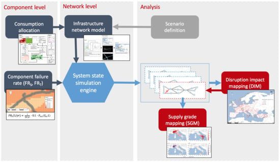
2. Materials and Methods

2.1. System and Data

The focus of this study is on the European natural gas infrastructure network, which consists of a number of interconnected components. Such a large-scale and complex infrastructure network is exposed to a variety of potential hazards, which can cause disruptions and result in loss of supply on a regional level [3]. In this study, a network perspective is employed to account for the complexity of the system. This includes geographic information (e.g., capacity of each pipeline segment, locations of infrastructure elements) required to model the system’s services. The next sections describe the various types of data collected and subsequently used in the analysis.

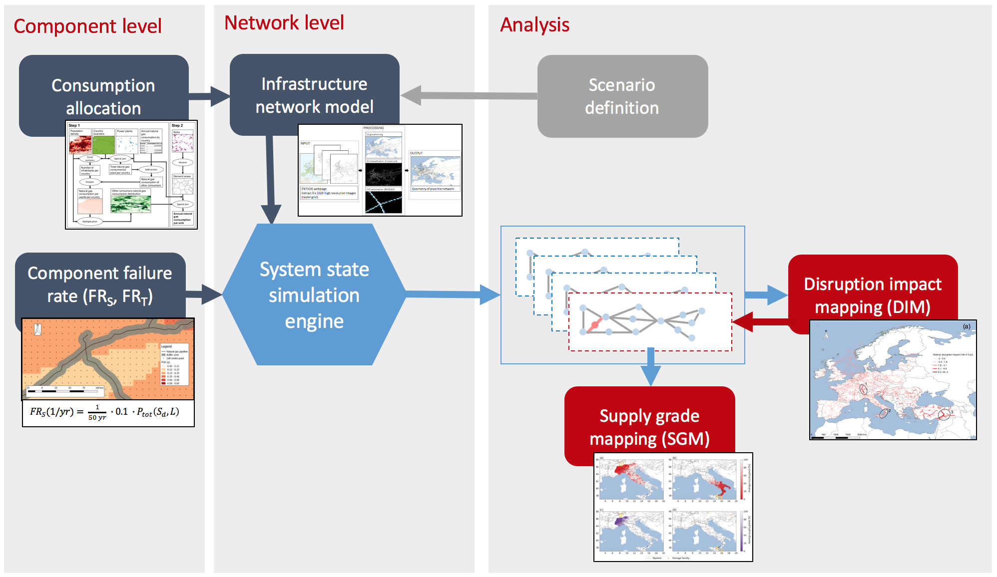
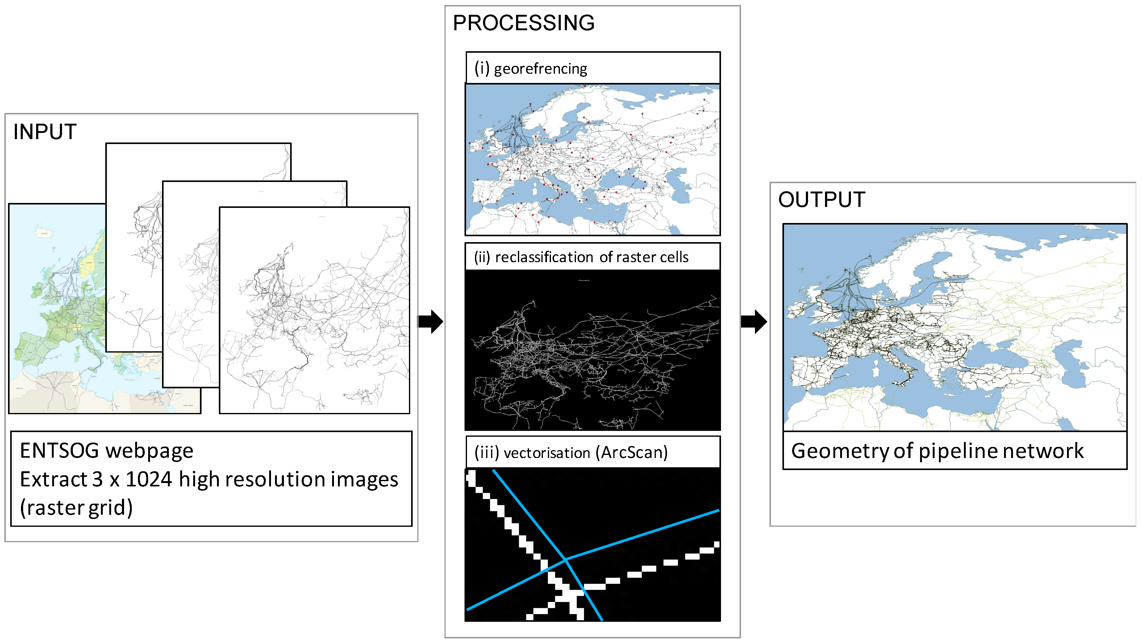
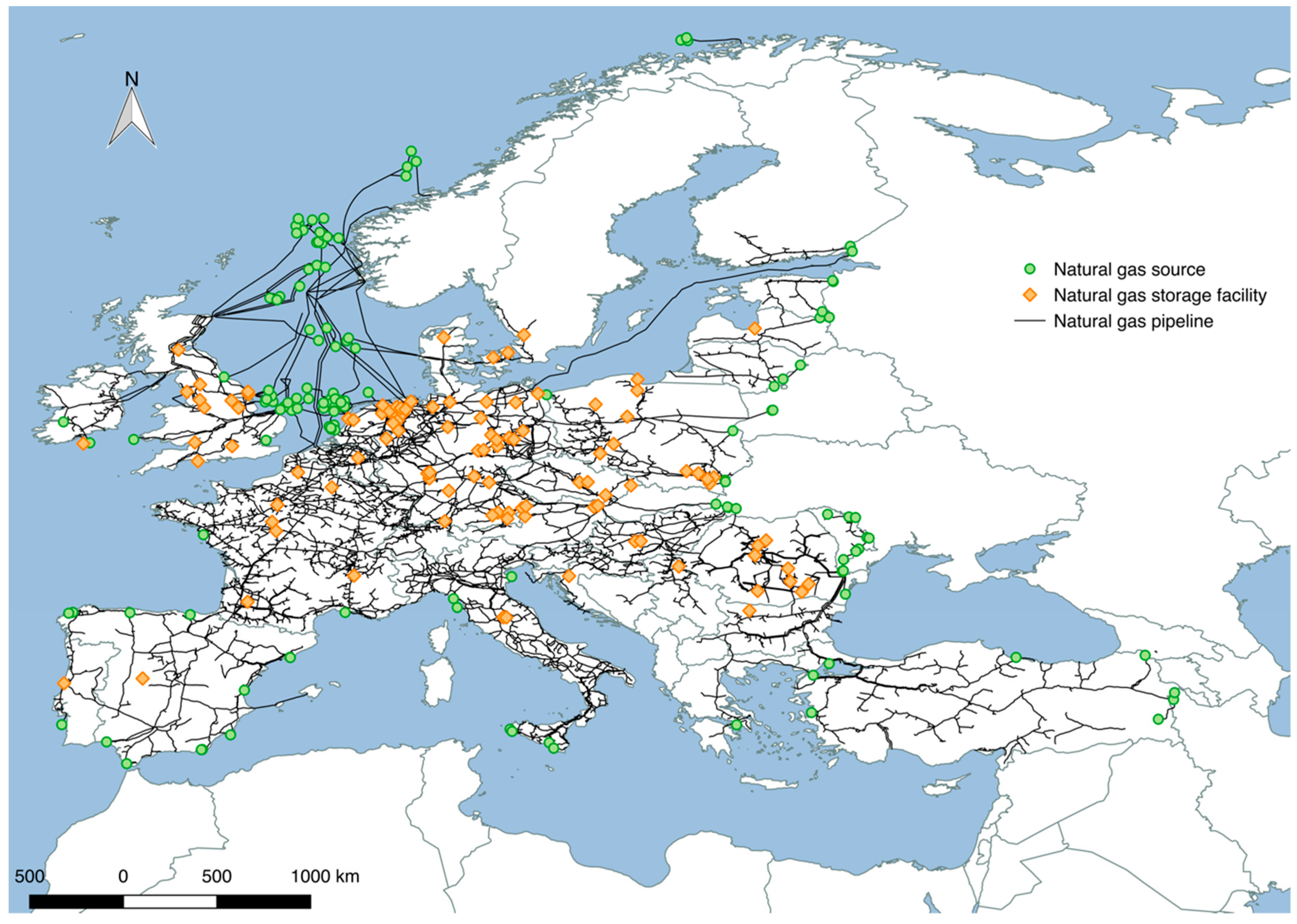
2.1.1. Infrastructure Network Data

A natural gas network consists of different components, such as pipelines, compressor stations, storage facilities, Liquefied Natural Gas (LNG) terminals to mention just a few [41]. The European Network of Transmission System Operators for Gas (ENTSOG) provides some essential information on the transmission network and its infrastructure. Table 2 gives an overview about the data and information used to develop the infrastructure network model developed in this study.
The geographic information of the European natural gas network was extracted from the ENTSOG’s transparency platform [42]. The three pipeline layers available (“medium and large pipelines” (>24 inch), “large pipelines” (>36 inch) and “all pipelines” (all pipelines recorded on the ENTSOG transparency platform)) were downloaded in form of 1024 high-resolution images (raster grid) for each layer as displayed in Figure 1.
Since the ENTSOG maps are in an unknown coordinate system, the maps have to be georeferenced. The information processing is similar to Jensen and Pinson 2017 [37] and illustrated in Figure 2. First, 78 georeferenced points evenly distributed throughout Europe (see Figure 2, (i) georeferencing) were chosen according to identified “Landmark” points of the network. The georeferencing transformation type “Thin Plate Spline” was applied to georeference the ENTSOG maps. The resulting georeferenced images, were then reclassified to achieve binary cell values (0 or 1, see Figure 2, (ii) reclassification of raster cells). This is done because the ArcScan tool requires a binary raster grid. Finally, to vectorize the raster grid, the ArcScan function provided by ArcGIS was used [2]. The default vectorization settings were applied, as they provide a satisfactory vectorization. To result in the different pipeline diameters provided by ENTSOG (in Figure 1), the three georeferenced vector files were combined.
This processing resulted in a dataset with information on geography and pipeline diameter. The required flow capacity was estimated for the three pipeline diameter bins defined in Table 3, using the average pipeline capacity for the European natural gas network [6]. Table 3 gives an overview of the pipeline categorization according to the diameter and capacity. The scales of the model and the data preciseness determine what phenomena can be examined. Although the pipeline capacity is roughly assigned according to three capacity bins because of the limited information provided by ENTSOG 2016 [42], the annual flows of the fully operational network can cover the allocated annual natural gas consumption. The rough allocation of pipeline capacities, due to the given pipeline diameter bins, however, does not allow to develop a detailed model of pipeline packing (the process of adding flow capacities due to short-term operational pressure increase of natural gas pipelines). The assigned pipeline capacities, however, could also represent the potential short-term capacity increase as they are roughly assigned with an upper limit.
The geographic information about natural gas storage facilities were extracted using the ENTSOG’s Application Programming Interface (API) to access the transparency platform [42]. To identify the natural gas sources the “Transmission Capacity Map 2015” of ENTSOG was used [42].
The flow in the network is facilitated by compressor stations. The compressor stations create a pressure gradient needed for an efficient natural gas transmission. Hence, compressor stations have to be considered for a meaningful disruption performance assessment of a natural gas network. However, no data on compressor station locations is available from ENTSOG. This gap was filled by assuming an uniform distribution of compressor stations along each pipeline, because a significant transport cost reduction can be achieved by an efficient compressor station arrangement [43]. In the case of technical failures, the compressor station failures are involved in the accident statistics and can be assigned according to the pipeline length. In the case of seismic hazards an exposure analysis of the corresponding pipelines (including compressor stations) is required. The location of a compressor station is estimated using an average distance between compressor stations along the pipelines. According to the reviewed literature, the compressor station distances range between 64 km and 424 km, as illustrated in Figure 3.
The compressor station distances, however, are very sensitive to the seismic failure rate as shown in SI Section S1: Seismic failure rate. Therefore, the smallest compressor station average distance found in the literature (64 km) [43,44,45,46,47,48,49] is conservatively taken for further analysis (Supplementary Materials).
The assembled infrastructure information is displayed in Figure 4. The data is imported to GIS (i.e., QGIS [50]) to provide a graphical representation of the European natural gas network.
A very important aspect is the information and accuracy of the location of the natural gas sources and natural gas storage facilities. The offshore sources and the sources resulting from LNG terminals, and import pipelines are given by the ENTSOG transparency map and trade statistics [51], respectively. The storage facility information is collected from the ENTSOG transparency platform. The storage facilities have a dual role in the natural gas system as they can consume natural gas (storage filling) or supply natural gas (storage withdrawal). Depending on the location in the network, a storage facility can support up to the total natural gas flow loss in case of a pipeline failure [41]. For this reason, the effects of the storage facilities are in particular examined.

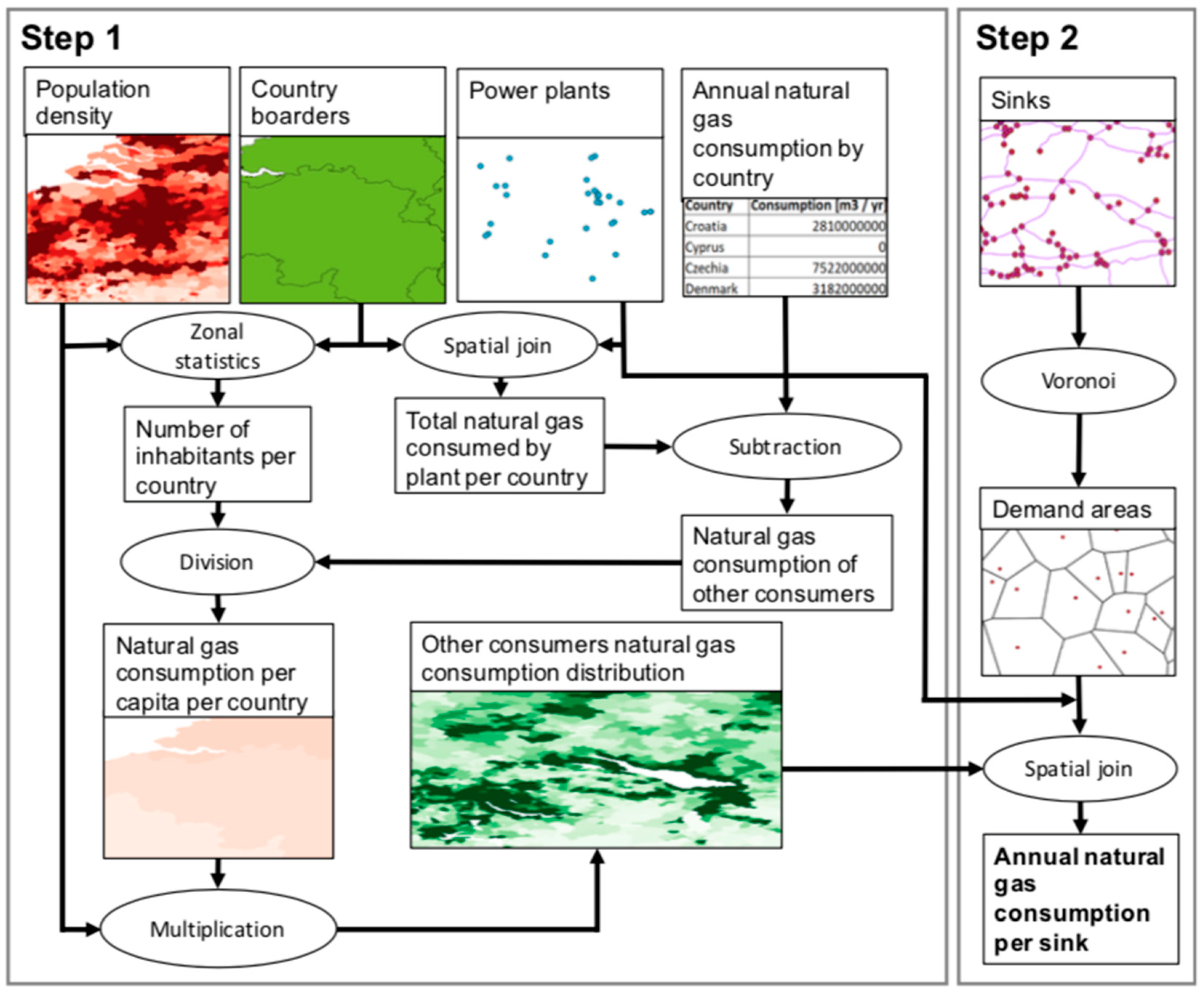
2.1.2. Data to Allocate the Natural Gas Consumption

To allocate the natural gas consumption throughout the network, the location and consumption of the natural gas power plants and the spatial distribution of the population is considered.
The employed datasets are listed in Table 4. The overall consumption on the national level is used and further allocated to power plants and other consumers (e.g., private households, industrial facilities, commercial facilities). There is no official database recording the European power plants [37]. Therefore, the open-source Enipedia database [52] was chosen, because it connects to several other databases, such as the Global Energy Observatory database [53] and the European Pollutant Release and Transfer Register (E-PRTR) [54]. To estimate the natural gas consumption of each power plant recorded in the Enipedia database [52], the carbon dioxide emissions were considered (see also Section 2.2.1).

2.1.3. Natural Hazard and Technical Failure Data

In this analysis, seismic hazards and technical failures are considered. The seismic hazard map for Europe [57] is used to analyze the exposure of the infrastructure to earthquakes. The data is provided as a raster grid on a ~11 km resolution for a 10% probability of exceedance in 50 years of a certain peak ground acceleration (PGA). The given parameters are inputs currently required by almost all National Annexes of the Eurocode 8, a standard for the design of structures for earthquake resistance [58]. An average lifetime of natural gas infrastructure system components is used to assess the total seismic hazard exposure and the mean annual seismic failure rate of that component and the network.
The Energy-related Severe Accident Database (ENSAD) [22,23,59] is used for the estimation of technical failure frequencies of natural gas accidents. ENSAD is part of a long-term research activity on comparative risk assessment at the Paul Scherrer Institute (PSI). It contains ~24,000 unique energy-related accident records worldwide, with more recent years under verification. The database is continuously updated using a full-chain approach, recording accident information (e.g., date, location, infrastructure type, accident type, energy chain and stage, fatalities, injuries, economic loss, etc.). The database is one of the most authoritative sources for consistent and worldwide information on accidents in the energy sector [59,60] and it is currently transformed into an interactive, GIS- and cloud-based, responsive web application [23,61]. For this study, the records reporting natural gas accidents involving the natural gas network of Europe are considered.

2.2. Methods

To conduct a resilience assessment in the field of engineered system sciences (e.g., infrastructure), besides the hazard exposure and frequency analysis, the performance or functionality of components and the system throughout a disruptive event has to be modeled [15,62]. This involves the disruption phase (draw-down), including the simulation of the disrupted state of the system, and a recovery phase (draw-up) represented by the system performance over time [62,63]. The focus of this study is on the disruption phase, whereas in another study, in which two of the authors were involved, a simulation of the recovery phase was carried out [64]. Figure 5 provides a schematic overview of the applied models and analysis methods to map the disruption impact and the resulting natural gas supply grade for selected scenarios.
In the following sections, an overview of the models and the applied analysis methods is given. The models are assembled using the collected geospatial information (see Section 2.1). The consumption is allocated to the infrastructure components (Section 2.2.1) and an infrastructure network model is built (Section 2.2.2). The component failure rates caused by seismic hazards (FRS) and technical failures (FRT) are estimated (Section 2.2.3). The network performance in case of a component failure is then computed using a system state simulation engine (Section 2.2.4). Finally, the disruption impact mapping (DIM), which is essential to assess the system’s disruption performance, and a scenario-based supply grade mapping (with focus on Italy) are described in Section 2.2.4.

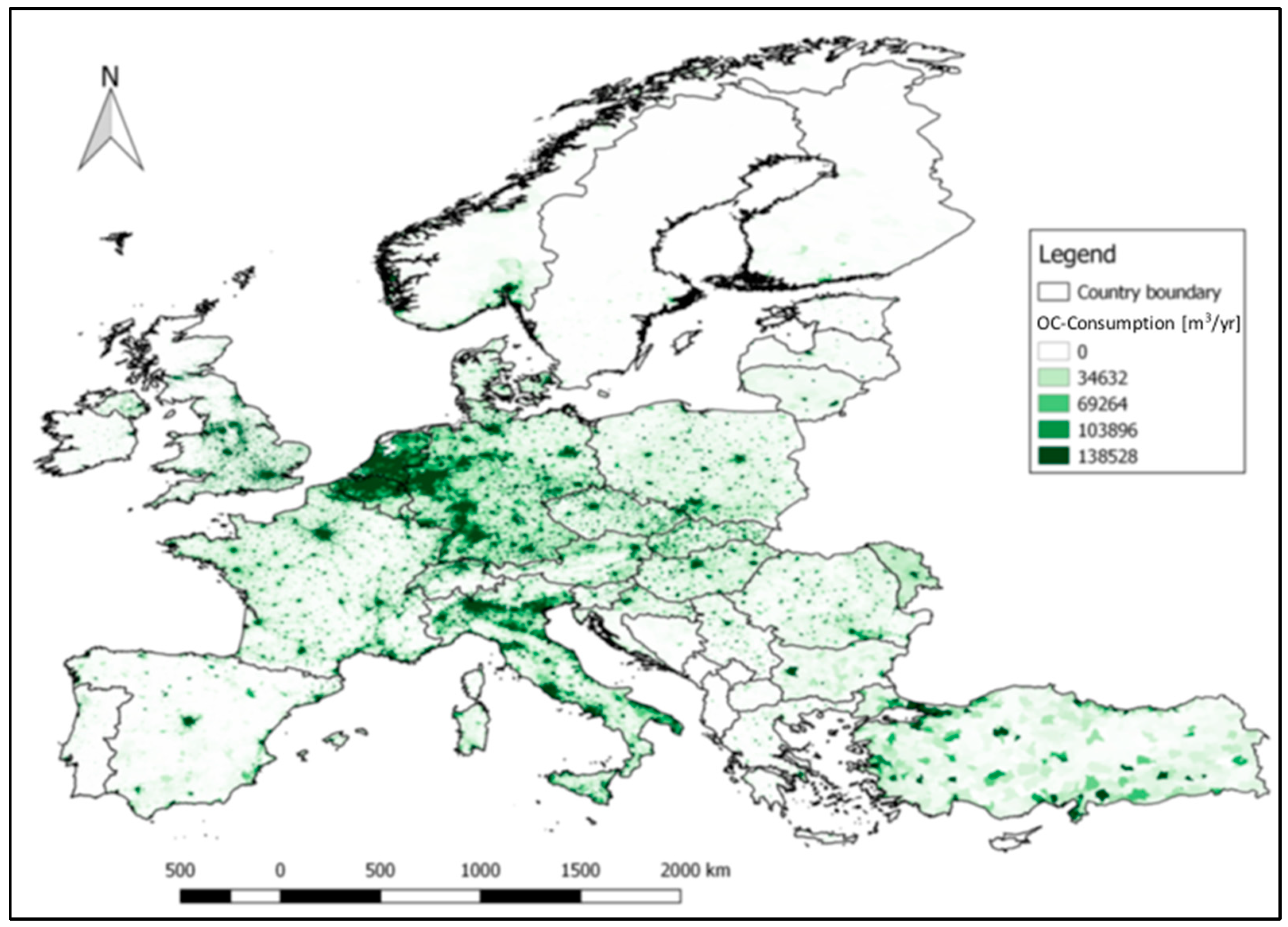
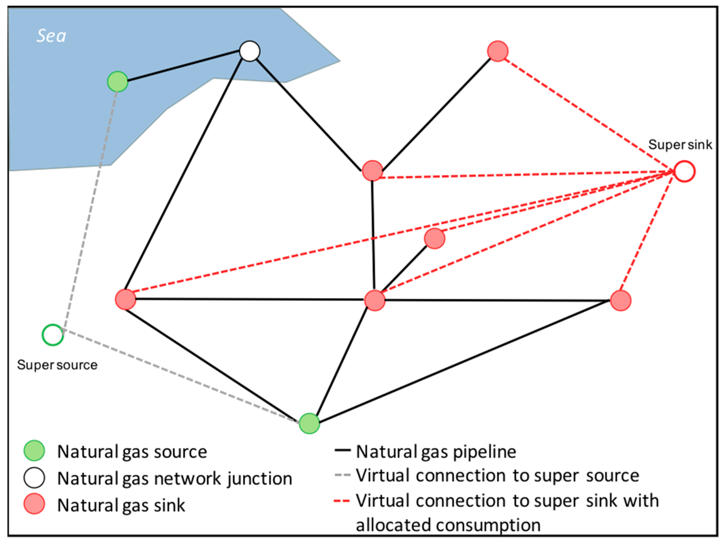
2.2.1. Consumption Allocation

The European natural gas network has the purpose to deliver natural gas to consumers throughout Europe. The service is represented by the maximum flow, because this is the amount of natural gas delivered to consumers. The consumers and the natural gas volumes consumed have to be geographically allocated to the network to account for the spatial distribution of the natural gas consumption. The consumers can be divided in two groups: natural gas power plants and other consumers (OC), such as private households, public bodies and private companies. A total of 23% of the natural gas is electrified by the natural gas power plants in Europe [65]. Since the large natural gas volumes consumed on a power plant level are concentrated at specific locations, the power plants need to be treated separately in the consumption mapping process. The remaining 77% of natural gas is consumed by OC, which use natural gas directly for heating and cooking and/or for industrial activities. The consumption is allocated according to the approach shown in the flow chart in Figure 6 [41].
The allocation process can be split in two steps. The first step (Figure 6, Step 1) involves the mapping of the natural gas consumption throughout Europe according to the population distribution and the power plant locations.
The Enipedia database [52] provides information on the natural gas power plant locations and associated carbon dioxide emissions. Hence, the natural gas consumption can be derived from the carbon dioxide emissions mCO2,PP [66,67] representing the effective production of the power plants in kg on an annual basis. The annual consumed natural gas volume CPP was estimated according to the combustion reaction of natural gas given in Equation (1) [66]:
0.9696 CH 4 + 0.0137 C 2 H 6 + 0.0167 residues 0.9833 CO 2 + residues ,
Only gas components with a molar fraction over 1% are considered. The molar number of CO2 atoms nCO2,comb built by the combustion of one mole of natural gas atoms nNatural gas,comb is given in Equation (2):
n N a t u r a l   g a s , c o m b   n C O 2 , c o m b = 1 0.9696 + 2 · 0.0137 = 1.003
.
This mole fraction results from a C atom conversion of the natural gas combustion reaction. CPP is calculated by applying the ideal gas law under standard conditions (T0 = 288.15 K, patm = 101325 Pa, R = 8.314 J/(mol K), Equation (3):
C P P = m C O 2 , P P M W C O 2 · n N a t u r a l   g a s ,   c o m b n C O 2 , c o m b · R · T 0 p a t m ,
where MWCO2 is the molar weight of carbon dioxide (44.01 g/mol) [67]. The total amount of natural gas consumed in a country by natural gas power plants CPP,country is found by summing up the CPP of all power plants j within the country boundaries (Equation (4)):
C P P , c o u n t r y = j c o u n t r y C p p , j .
The estimated power plant consumption (Cpp,country) was compared to the European natural gas consumption of power plants by country [68]. With the presented method, roughly 60% of the natural gas consumed by power plants according to Eurostat 2018 [68] could be allocated to specific power plants in Europe.
The OC group consumption is the consumption of each country without the power plant consumption as given in Equation (5).
C O C , c o u n t r y = C t o t , c o u n t r y C P P , c o u n t r y ,
where Ctot,country is the natural gas consumption by country provided by the International Energy Agency (IEA) [1]. The natural gas power plant consumption by country (CPP,country) is estimated in Equation (4) and COC,country is the natural gas consumption of the OC by country. To allocate the COC,country to the population density, a scaling factor fscale,country is estimated according to Equation (6):
f s c a l e ,   c o u n t r y = C O C , c o u n t r y P c o u n t r y ,
where Pcountry is the population by country estimated from the European population GIS raster [55]. A linear relationship between the OC and the population distribution is assumed to downscale the natural gas consumption. Therefore, the natural gas consumption for each raster cell i can be estimated according to Equation (7):
C i = f s c a l e ,   c o u n t r y · P i ,
where Pi is the population of each raster cell and is provided by the European population GIS raster [55] with the resolution of 30 arc-seconds (−1 km). The OC consumption map is displayed in Figure 7. The colour of cell i represents the annually consumed volume of natural gas (Ci) within this particular raster cell.
The second step (Figure 6, Step 2) involves the building of the consumption areas, i.e., a division of the land area according to the identified sinks of the network. Sinks are all the network points (e.g., junctions) on land, which are not identified as sources (e.g., consumer vertices). It is assumed that the natural gas consumption can be allocated to the closest natural gas sink of the network. This assumption is similar to previous studies, where the number of people connected to the network instead of the consumption volumes have been considered [7,8]. The assumption, however, allows applying a Voronoi algorithm (also called Thiessen algorithm). The algorithm cuts the nearest neighbor connection lines of the sinks rectangular into half and therefore creates subareas, containing one single sink each [69]. The consumption of each sink is found by summing up the mapped OC and the power plant consumption for the corresponding area. The consumption year is set to 2015 because the population density is also provided for the year 2015. However, the natural gas power plant consumption from the Enipedia database [52] stems partially from a previous project, which was recording carbon emissions from 2012. In this context, as a first approximation, these emissions have been allocated to 2015, since the natural gas consumption for the thermal power stations is on the same level [68]. Finally, seasonal consumption differences throughout a year are neglected as the pipeline flow capacity was based on an annual average.

2.2.2. Infrastructure Network Model

Complex networks approaches are employed to capture the non-trivial topological features of the European natural gas network (e.g., the natural gas sources and sinks are interconnected and distributed in space). The approaches are proved to address the study objectives, because the infrastructure network can be simplified while important features such as the network topology are retained [41,70]. The geographic information of the European natural gas network is transformed into a connected and undirected weighted graph G(V,E,c) with no loops [3]. The vertices V can be identified as sinks (e.g., consumer vertices), sources (e.g., natural gas production platforms, LNG import terminals, and import pipelines) or nonfunctional junctions as for instance junctions in the sea (see also Section 2.2.1). The edges E(u,v) represent the pipelines connecting between Vu and Vv. Furthermore, c(u,v) represents the assigned flow capacity for each edge, while f(u,v) indicates the computed flow in the network.
To estimate the flow in the graph, a maximum flow estimation (Equation (8)) using the Ford–Fulkerson algorithm is applied as it is considered to represent the operators’ behavior in case of a crisis [33]. The Ford–Fulkerson algorithm is a meaningful algorithm to investigate the European natural gas supply through its network, as it considers the distance of the source to the sink. The algorithm does not consider political aspects or detailed natural gas market developments, but it considers the transportation cost in the sense that the sinks closest to the source will be served first. For all these reasons, the algorithm is popular and often applied [30,33]. The algorithm estimates the largest possible flow from a single source s to a single sink t [71]. The basic idea of the Ford–Fulkerson algorithm is to find paths p(s,t) from s to t with unexploited capacities, while the capacity constraint (Equation (9)), the flow conservation (Equation (10)) and the skew symmetry (Equation (11)) must be fulfilled.
F m a x = u t f ( u , s ) = u V f ( t , u ) ,
f ( u , v ) c ( u , v ) ,
u V : u s   a n d   u t f ( u , v ) = 0 ,
f ( u , v ) = f ( v , u ) ,
The search is repeated until no additional flow can be added. For the search the Boykov–Kolmogorov algorithm is applied, because it is the fastest algorithm available to conduct this kind of analysis [72]. The European natural gas network, as well as the resulting graph G, has multiple sources and sinks. To convert the multiple source/sink problem to a single source/sink problem, a super source s* and a super sink t* are introduced. Figure 8 illustrates conceptually this transformation. The estimated consumption volumes (see Section 2.2.1) of each sink can be allocated to the network as capacities of the connection to the super sink t*. For the flow simulation of the network, MATLAB [73] and and/or Python’s igraph library [74] and corresponding packages were used.

2.2.3. Component Failure Rate

Natural gas networks are exposed to many potential disruptive events, of which seismic hazards and technical failures were identified to cause medium to high risks [39]. Therefore, in this section, the estimation of the component failure rate caused by seismic hazards (FRS) and the technical failure rate (FRT) is introduced.
To estimate the component failure rate caused by seismic hazards (FRS), the seismic hazard exposure of each component is assessed and combined with the corresponding fragility curve. The exposure of the natural gas network components to seismic hazards is estimated using the seismic hazard map displayed in Figure 9.
The map provides values of Peak Ground Acceleration (PGA) with a 10% probability of exceedance in a 50-year period. The specific PGA value is given for each pixel cell on a geospatial resolution of approximately 11 km.
The exposure analysis involves the PGA of a likely earthquake at the geographic location of each component. The PGA of the closest raster cells for each component are averaged using a buffer zone around the corresponding component. The width of the buffer region is defined as the diagonal of a raster cell. This ensures that at least one earthquake hazard map raster cell center point is present in the buffer region. Figure 10 illustrates the seismic hazard analysis, including the applied buffer zone.
The seismic fragility for infrastructure components is measured by fragility curves, which relate to the probability of reaching at least a particular damage state for a given excitation level. The fragility curves were computed following the HAZUS 2003 [19] framework. Thus, the specific failure probabilities of the pipelines PPipelines (Sd,L) and the compressor station PCompressor (Sd,ds = 3) can be estimated.
To estimate the fragility curves of natural gas pipelines, the PGA (for compressor station fragility) and the Peak Ground Velocity (PGV) (for the pipeline fragility) values are required. Therefore, a given PGA is converted to PGV using a relationship between PGA and PGV, called Peak Ground Motion (PGM) parameters and the ground motion intensity (INT) in terms of modified Mercalli intensity, as presented in Caprio et al., 2015 [75]. It is important to note that this is an approximation, since a linear relationship between PGA and PGV is assumed. However, the presented relationships were chosen because they apply for all European countries and because the INT–PGM relations are statistically robust. Caprio et al., 2015 [75] provides global regression relationships of INT and the peak ground motion (PGM), given in Equations (12) and (13).
I N T = α 1 + β 1 l o g 10 ( P G M ) i f   l o g 10 ( P G M ) t P G M ,
I N T = α 2 + β 2 l o g 10 ( P G M ) i f   l o g 10 ( P G M ) > t P G M ,
where PGM can either be PGA [cm/s2] or PGV [cm/s]. Table 5 provides the regression coefficients (α and β) as well as the threshold tPGM, used in the conversion equations. The PGV can be calculated from the PGA, combining both equations. First, Equations (12) or (13) is used to estimate the INT using the PGA from the exposure analysis and the parameters for PGA from Table 5. Then the Equations (12) and (13) are transformed to Equations (14) and (15).
P G V = 10 I N T 1 β 1 i f   I N T 4.9 ,
P G V = 10 I N T 2 β 2 i f   I N T > 4.9 ,
Using Equations (14) and (15) with the estimated INT for the PGA and the corresponding parameters for PGV from Table 5, the PGV can be estimated.
The fragility curves for the natural gas pipelines are modelled using an empirical relation of the expected repair rate (RR) due to a certain excitation given in PGV. The definition of the repair rate can be found in Equation (16):
R = k · 0.0001 · P G V 2.25 .
RR depends on the pipeline material represented by k. Old welded steel pipelines are classified as brittle pipelines (k = 1), while pipelines with submerged arc welded joints are called ductile pipelines (k = 0.3). To be on the conservative side brittle conditions (k = 1) are assumed as done in other studies [7,8]. In Equation (16) both damage states “leaks” and “breaks” are taken into account. When a pipeline is damaged due to seismic wave propagation (governed by PGV), the type of damage is likely to be a leak. In HAZUS 2003 [19], it is assumed that damage due to seismic waves will consist of 80% leaks and 20% breaks. The resulting RR can then be used to estimate the pipeline fragility curve as given in Equation (17):
P p i p e l i n e ( D S > d s | S = S d ) = 1 exp ( R R · L ) .
According to HAZUS 2003 [19], each compressor station fragility curve for a given damage state ds (e.g., slight, moderate, extensive, complete) is characterized by the median peak ground acceleration μ and peak ground acceleration dispersion β. The probability of reaching at least the damage state ds for a given excitation Sd, in terms of peak ground acceleration (PGA), is given in Equation (18):
P c o m p r e s s o r ( D S > d s   | S = S d ) = Φ ( 1 β l n ( S d μ ) ) ,
where Φ is the standard normal cumulative distribution function given in Equation (19):
Φ ( x ) = 1 2 + 1 2 erf ( x 2 ) .
A moderate damage state ds3 and unanchored compressor conditions are assumed as the lowest damage state where a shutdown of the compressor station can be expected. Namely, this compressor damage state is described in HAZUS 2003 [19] as: “considerable damage to mechanical or electrical equipment or building”, with µ = 0.24 and β = 0.6.
Using the developed infrastructure model, the compressor stations are uniformly distributed along the pipelines (see Section 2.1), and allocated to the pipelines according to Equation (20):
n = L / Δ L ,
The pipeline length and the average distances of the compressor stations are represented by L and ΔL, respectively (see also Section 2.1.1). The overall pipeline failure probability Ptot(Sd, L) can be estimated as given in Equation (21). Hence, the analysis of single pipeline failures considers compressor stations.
P t o t ( S d ,   L ) = 1 ( ( 1 P P i p e l i n e ( S d ,   L ) ) · ( 1 P C o m p r e s s o r ( S d ,   d s = 3 ) ) n )
The mean annual seismic failure rate FRS of a network component for a seismic excitation Sd, given by the hazard map, is defined in Equation (22):
F R S ( 1 / y r ) = 1 50   y r · 0.1 · P t o t ( S d ,   L ) ,
where 50 years and the factor 0.1 are resulting from the given information of the seismic hazard map (10% exceedance probability in a 50-year period) [57].
The estimation of the mean annual technical failure rate (FRT) is a result of the exposure of the infrastructure combined with the historical number of accidents recorded in ENSAD. The exposure of a pipeline to technical failures is defined as its length Ltot multiplied by the exposed time according to Equation (23):
Exposure   [ k m · y r ] = t = 1990 t = 2013 L t o t ( t )   d t .
The temporal change of Ltot is not known for the system under investigation. Therefore, the reported temporal change in the total length of the European gas transmission system of the European Gas pipeline Incident data Group (EGIG) is used as a proxy because it represents seventeen major gas transmission system operators in Europe [76]. The change of the total pipeline length over time Ltot is modeled, assuming that Ltot grows with the same growth rate as the total length of the EGIG pipeline network throughout the defined time window. Equation (24) shows the time dependent Ltot of the pipeline network.
L t o t ( t ) = A · t + B ,
The gradient A is calculated from the linear fit of the EGIG pipeline growth. The offset B is found by inserting the total pipeline length of the network under investigation for the reference year.
All the available historical accident information on the pipelines and compressor stations in ENSAD from 1990 to 2013 were used (107 recorded pipeline accidents). This time window was chosen because the temporal change of the natural gas network reported by EGIG 2015 [76] experienced significant step changes around the 1990, corresponding to new members joining EGIG. The technical failure rate FRT’ is estimated according to Equation (25).
F R T [ 1 k m · y r ] = N A c c i d e n t E x p o s u r e ,
The accident number NAccident is aggregated at the European level because no significant differences in FRT’ are expected as the natural gas transportation is regulated and standardized on a supranational level. The role of ENTSOG, for example, is to set out the rules for system operation covering subjects such as operational security (e.g., inspection and maintenance practices) [42]. The resulting FRT’ is in the same magnitude as reported by other databases [70]. The pipeline specific FRT is finally estimated according to Equation (26) with L representing the pipeline length:
F R T ( 1 / y r ) = F R T · L ,

2.2.4. System State Simulation Engine

As pipeline networks can compensate single pipeline failures due to capacity redundancies or storage facilities, an assessment of a single pipeline disruption results in a non-trivial topological complex network problem [77]. To characterize a disruption resulting from a particular location of the network, the combination of the failure rate FRX, representing either the FRS or FRT of the corresponding pipeline, and the severity of the impact is applied. The impact represents the loss of the system performance caused by flow capacity loss of a single pipeline failure. The failure rate FR is computed considering the different natural gas network infrastructure components (see Section 2.2.3). The flow loss in case of a failure of pipeline i, is estimated according to Equation (27).
Δ F m a x , i   [ % ] = F m a x F m a x , i F m a x · 100 % ,
where ΔFmax,i. represents the system performance loss in percent, while Fmax stands for the maximum flow in the fully operational network (see Section 2.2.2), which is in fact the total consumption of the region under investigation. Fmax,i is the maximum possible flow without the pipeline i. Hence, the estimation takes alternative natural gas flow routes of the network into account to meet the natural gas consumption.

2.2.5. Disruption Impact and Supply Grade Mapping

A disruption impact mapping (DIM) as well as a supply grade mapping are carried out.
The disruption impact DIM is computed using Equation (28).
D I M   ( % / y r ) = F R X · Δ F m a x , i ,
A smaller DIM value means lower impact on the supply service of natural gas. The resulting DIM for each pipeline i can be assigned to the corresponding pipeline and gives an indication of potential bottlenecks, taking storage facilities into account. The consideration of the failure rate provides further information about the expected frequency with respect to seismic hazards and technical failures.
Storage facilities can act as source (withdrawal of natural gas) or as sinks (filling of natural gas). As storage facilities, can be operated as sources or sinks, a scenario analysis is carried out twice to investigate the potential effect of such facilities to reduce the DIM in case of a single pipeline failure.
The supply grade mapping is carried out for selected pipeline failure scenarios once with and once without the storage facilities. The analysis is presented as graphical representations of natural gas supply grade. The supply grade (SGM) is the percentage of the sink’s consumption that can be covered in case of a pipeline failure. It is calculated for each supply area as shown in Equation (29).
S G M   ( % ) = S C A c · 100 % ,
where SC stands for the average sink’s natural gas flow. The estimated natural gas consumption of the corresponding consumption area is represented by AC. The Ford–Fulkerson algorithm allocates the natural gas flow on the geospatial network component level differently for each computation. Therefore, a Monte Carlo simulation is performed with 10’000 simulation steps computing the overall average flow for each supply area (Voronoi polygon). The maxflow algorithm of Python’s igraph package [74] based on the Ford–Fulkerson algorithm is used. The computationally intense simulation is performed using computing clusters (docker [78]) and multiprocessing. The supply change is below 1% after about 3500 simulation steps for all the computed average natural gas flows (see also SI Section S3: Monte Carlo simulation supply grade mapping) (Supplementary Materials). The goal of the simulation is not to conduct a precise quantification of the supply grade for a specific sink, but rather to give an overall insight to bottlenecks of regions.

3. Results and Discussion

In Section 3.1 the potential disruption with and without storage facilities is discussed taking seismic hazards and technical failures separately into account. The seismic and technical failure rates are compared in Section 3.1.3. Finally, selected scenarios to illustrate the computation of a possible supply loss on geospatial basis is given in Section 3.2.

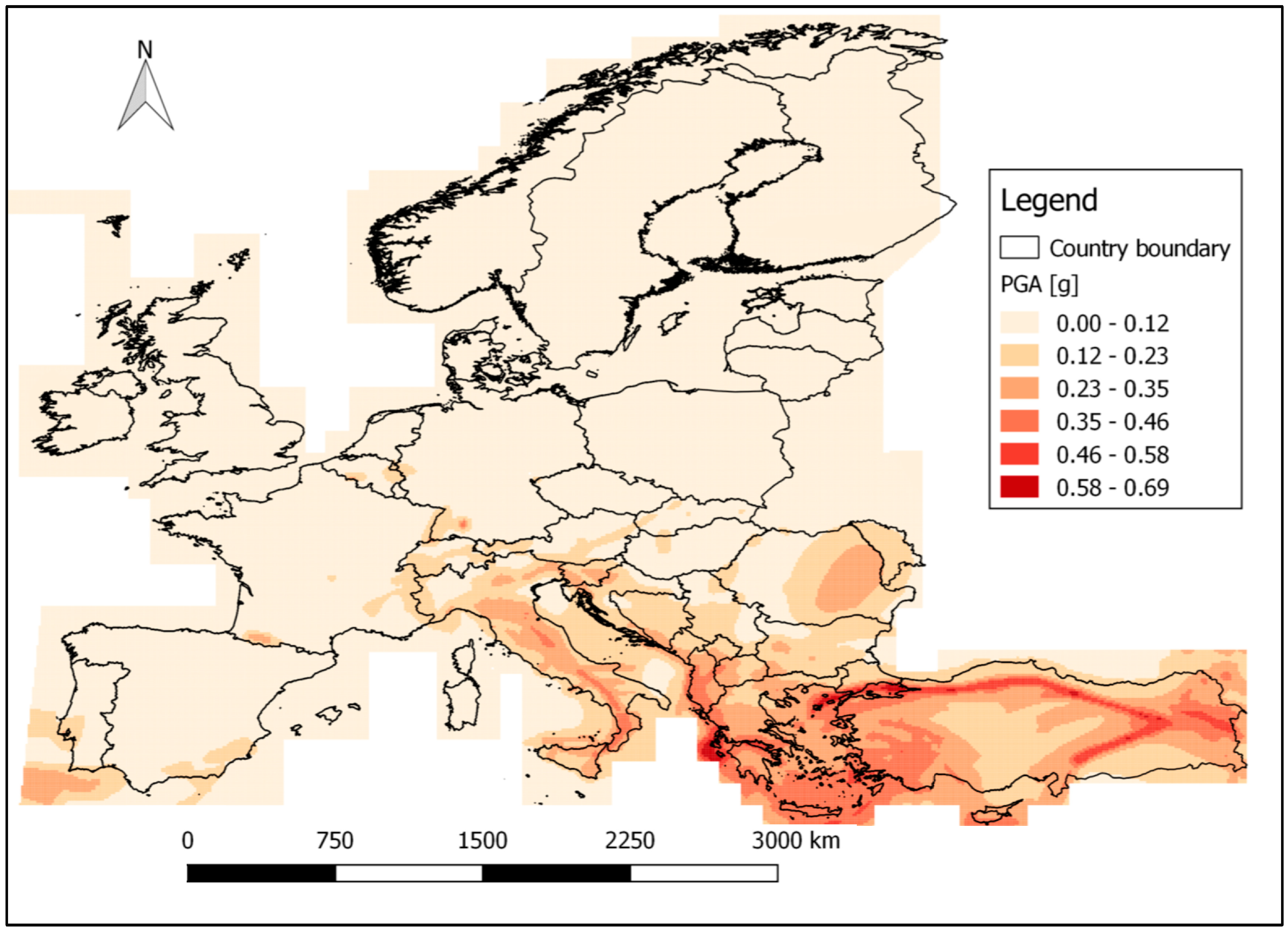
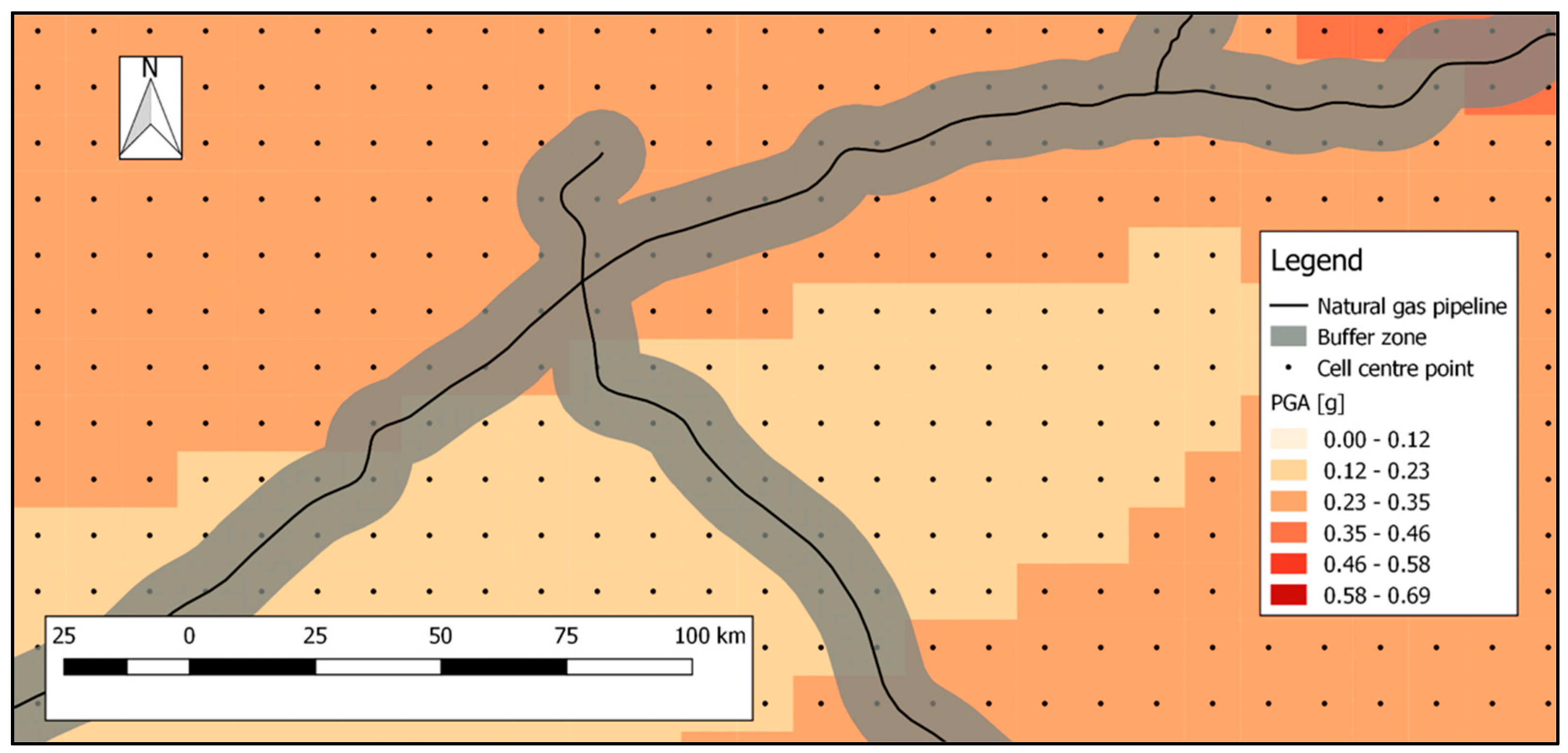
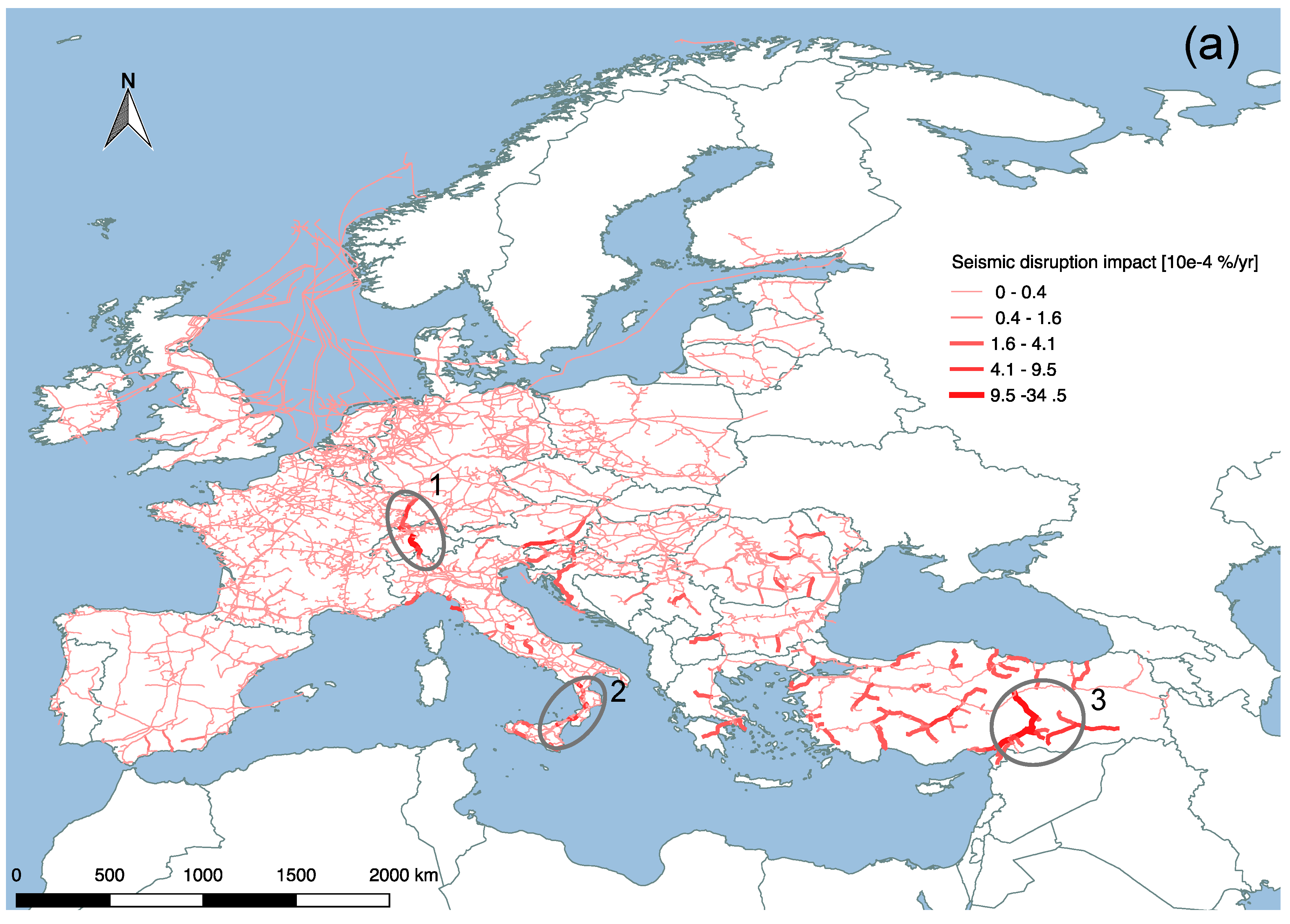
3.1. Disruption Impact Mapping

The DIM facing a single pipeline failure is discussed in this section for six pipelines (labeled 1 to 6) with a system performance loss (ΔFmax,i, see Equation (27)) higher than 1% (∼4.5 109 m3/year). The six pipelines are given in Table 6. The system performance loss is computed without the corresponding component using the system state simulation engine. For the discussion, not only the system performance, but also the exposure and the estimated failure rate is taken into account. The failure rates for each pipeline are estimated separately for seismic hazards and technical failures considering the exposure and the intensity.
These six pipelines are discussed in more detail with respect to seismic hazards and technical failures. Whereas the Index 1 represents the pipeline with the highest system performance loss, but not necessarily the highest overall DIM. The given pipeline index numbering is consistently applied for this discussion.

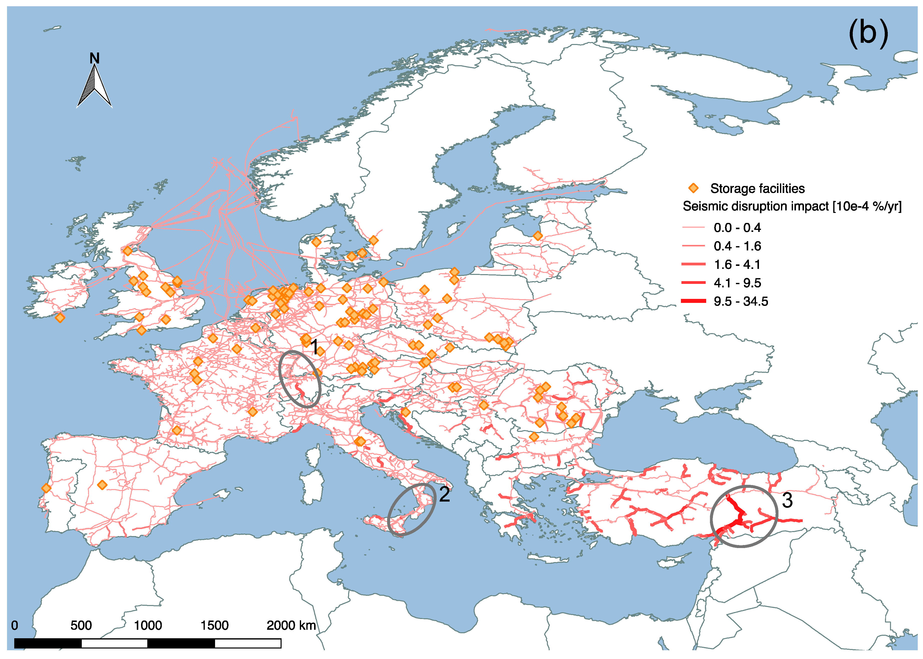
3.1.1. Seismic Disruption Impact Mapping

Figure 11 shows the disruption impact related to seismic hazards on the European level. In general, the pipelines in seismic active regions have relatively high disruption impacts due to the higher exposure. Pipelines with disruption impacts between 5 × 10⁻⁴ %/yr and 10 × 10−4 %/yr can be found all over Turkey, in the Swiss Alps and in the upper German Rhine rift region as well as in Southern Italy. Pipelines with disruption impacts between 1 × 10⁻⁴ %/yr and 5 × 10⁻⁴ %/yr are located from Southern and Northern Italy, along the alpine orogenic belt from Northwest Italy over Switzerland and Austria along the Dinarides (in Slovenia, Croatia, Serbia, Bosnia, Macedonia, Bulgaria and Greece), as well as in Romania and Spain. Figure 11b shows the disruption impact when storage facilities are considered to overcome potential supply shortages. Comparing Figure 11a,b shows that in general, storage facilities can compensate potential pipeline disruptions. The overall disruption impact can be reduced by 21% (only pipelines with DIM > 0 are considered).
The Swiss Alps and the upper German Rhine rift region are regions with low to moderate seismic hazard exposure [79]. The pipeline crossing the Swiss Alps (Figure 11, Index 1), however, results in a high DIM. The Transitgas pipeline and its southern extensions have the highest impact on the maximum flow in case of a failure. The pipelines connect Northern Italy via Gries Pass through Switzerland with the German and French natural gas networks [80]. The high maximum flow loss results from the fact that this pipeline is the only one crossing the central Alps providing a North/South connection. The seismic exposure and the corresponding seismic failure rate, on the other hand, is rather low (between 0.0 and 0.4 × 10⁻³/yr). Therefore, the high DIM is mainly driven by the system performance loss (ΔFmax,i). The withdrawal of natural gas from storage facilities located in Northern Italy can reduce the seismic DIM from 9.3 × 10⁻⁴ %/yr to 2.8 × 10⁻⁴ %/yr (Figure 11b, Index 1). As storage facilities cannot reduce the DIM to zero, this pipeline is investigated in Section 3.2.
The pipelines connecting Sicily and Calabria (Figure 11, Index 2) have the second highest impact on the maximum flow in case of a failure. The reason is that those pipelines are a part of the Trans-Mediterranean pipeline system [81] and the Green-Stream project [82] connecting Algeria, Tunisia and Libya with Continental Europe. These pipelines provide a major share of the natural gas consumed in Europe [6]. The pipeline was also identified by ENTSOG in corporation with the Gas Coordination Group as one of the emergency supply corridors [83]. The pipeline, however, is exposed to seismic active zones in Southern Italy [79]. A potential disruption of this important route by such a hazard can only be partially compensated with storage facilities. Moreover, a similar scenario analysis (disruption of natural gas from Algeria) conducted by ENTSOG [83], results also in supply shortages for Italy, Slovenia and Croatia. The withdrawal of natural gas from storage facilities located in Northern Italy can reduce the seismic DIM from 9.0 × 10⁻⁴ %/yr to 2.3 × 10⁻⁴ %/yr (Figure 11b, Index 2).
All pipelines with disruption impact higher than 10 × 10−4 %/yr are located in southeastern Turkey. The maximum DIM caused by seismic hazards amounts to 34.5 × 10⁻⁴ %/yr, which is the pipeline with Index 3 in Figure 11. The Turkish pipeline between the cities Silvas and Malatya connects the southeastern part of Turkey with the Trans-Anatolian pipeline. The Trans-Anatolian pipeline transports natural gas from Georgia and Iran towards the West, as for example to Ankara and beyond [84]. The high DIM results from the fact that on the one hand, the whole natural gas consumption of Southeast Turkey is provided solely by this pipeline (dead-end pipeline). On the other hand, the DIM is a result of the seismic highly active Eastern Anatolian fault zone. Since there is no storage facility, according to ENTSOG 2016 [42], in this region, the DIM cannot be compensated by storage facilities (see Figure 11b, Index 3).
The other high flow pipelines (Indices 4 to 6) are not exposed to seismic hazards according to the exposure analysis. Hence, the pipelines result in no seismic DIM and are not indicated in Figure 11.

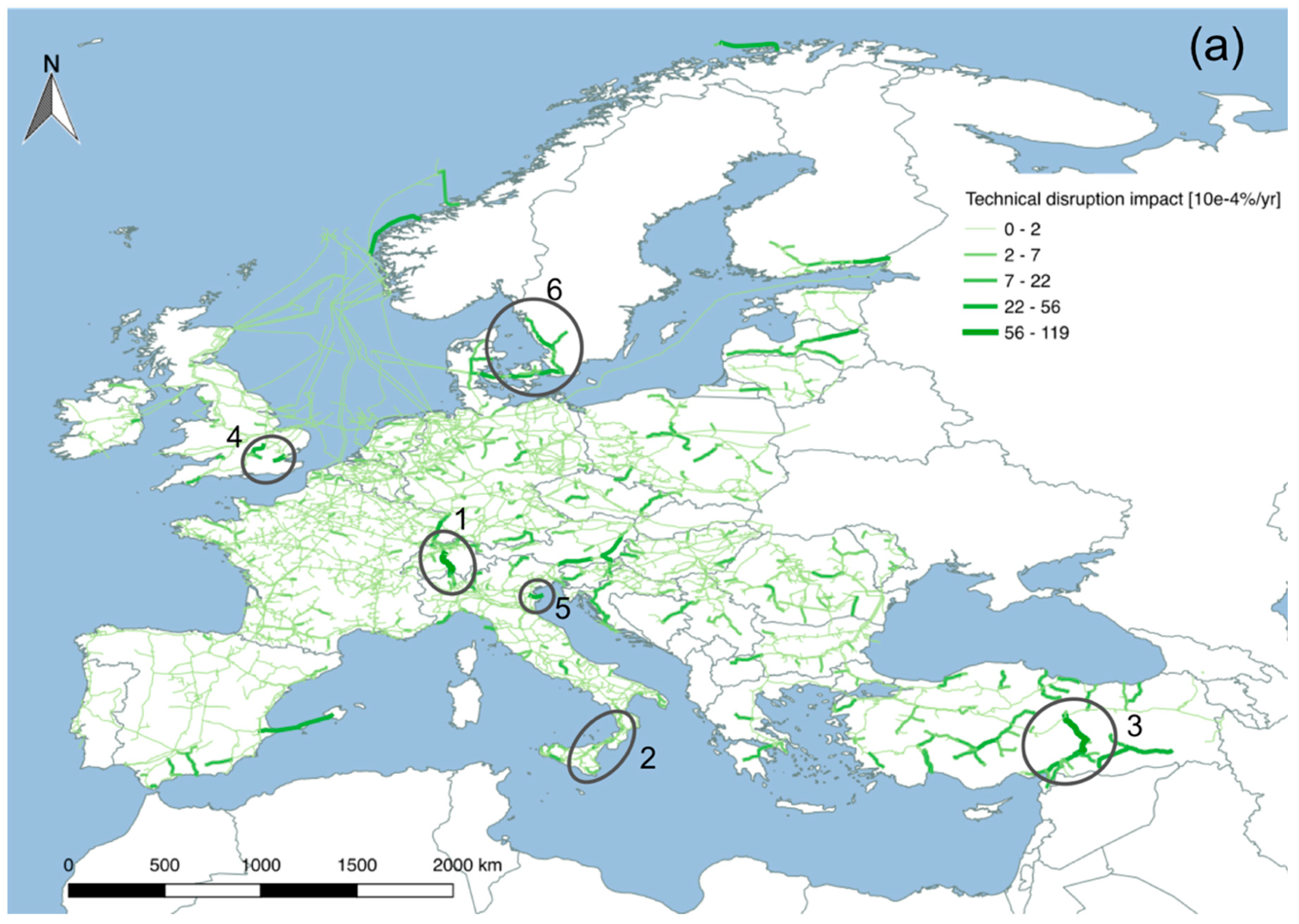
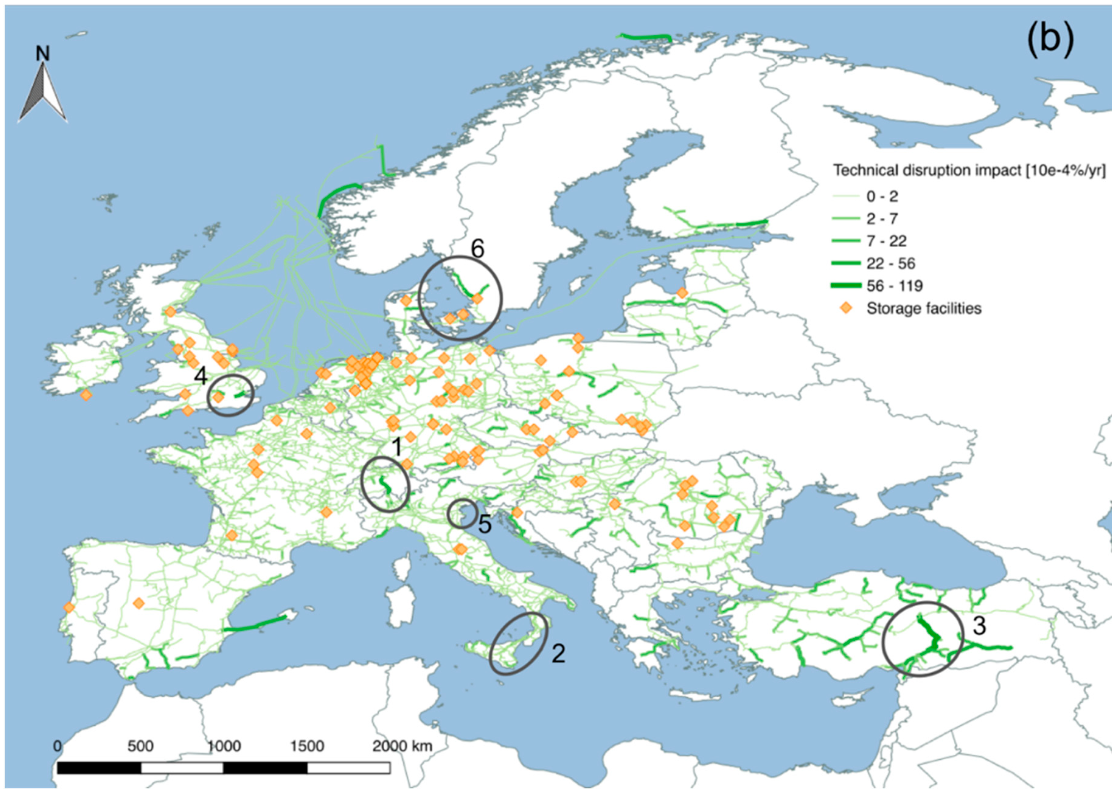
3.1.2. Technical Failure Disruption Impact Mapping

The disruption impact related to technical failures is shown in Figure 12. Pipelines with high disruption impact are occurring throughout Europe. Such pipelines are found for instance in the Norwegian and Mediterranean Sea as well as at the border with Russia. Because the FRT is pipeline length dependent, a high disruption impact is also rather related to long pipelines. As in the case of seismic hazards, comparing Figure 12a,b shows that the storage facilities can reduce the disruption impact.
High DIM values related to technical failures are computed for the natural gas pipeline crossing the Alps and the Trans-Mediterranean pipeline system [81] connecting Algeria, Tunisia and Libya with Continental Europe (see Figure 12, Index 1,2). Similar to the seismic DIM, this result is driven by the high system performance loss in case of a failure. The absolute DIM value for this pipeline, however, is ~10 times higher in case of technical failures compared to the seismic failures (see also Section 3.1.2). In case of an outage, the flow in the affected pipelines cannot be fully compensated by storage facilities (see Figure 12a,b Index 1,2), and therefore are further investigated in Section 3.2.
The highest technical DIM amounts to 118.4·10−4 %/yr. The corresponding pipeline is a dead-end pipeline providing natural gas to a large part of the South-Eastern part of Turkey (see Figure 12, Index 3). As it is a dead-end pipeline with no storage facilities in its supply region, a potential outage caused by a technical failure cannot be compensated.
Two pipelines in the Region of London cause a high system performance loss (see Figure 12, Index 4). The high impact of the southeastern pipeline results from the fact that it is the only high capacity pipeline delivering natural gas to London and surrounding area. The high system performance loss of the northwestern pipeline can be explained as it is the only high capacity pipeline, delivering natural gas to the administrative region of southwest England. Moreover, both pipelines are modelled as dead-end pipelines without any storage facilities in the supply area. Therefore, a potential outage caused by a technical failure cannot be compensated.
The pipeline near Venice (see Figure 12, Index 5) connects the LNG port Cavarzere Porto Levante with the Italian mainland [85]. The high system performance loss leads to the conclusion that the Cavarzere Porto Levante constitutes a strategical important natural gas source to cover the European natural gas demand. The system performance loss combined with the length of the pipeline, causing a rather high FRT, leads to the high DIM. Using storage facilities (see Figure 12b, Index 5), however, could compensate a potential failure of this pipeline.
The pipeline connecting the European mainland with the Danish Islands Funen and Zealand results in a high system performance loss (see Figure 12, Index 6). The pipeline ends at Copenhagen, from where one single pipeline heads to Sweden. The high system performance loss results because it is the only pipeline supplying Copenhagen and Southern Sweden with natural gas. The supply losses can be compensated by storage facilities. The related infrastructure components were also identified by ENTSOG [83] as a critical natural gas supply scenario.

3.1.3. Comparison of Seismic and Technical Failure Rates

The comparison of mean annual seismic and technical failure rates (FRS and FRT) and the corresponding disruption impact is listed in Table 7. The failure rates are estimated separately, i.e., there is no combining of seismic and technical hazards. The analysis shows that the failure rate caused by technical hazards are higher than the ones caused by seismic hazards (due to the event frequency and exposure). The highest mean annual technical failure rates occur throughout Europe, while high mean annual seismic failure rates can be found in the seismic active zone in southeastern Europe. The estimated failure rates plotted against the estimated system performance losses for each pipeline can be found in SI, Section S2: Comparison of mean annual seismic and technical failure rates (Supplementary Materials). Moreover, comparing the estimated mean annual seismic and technical failure rates to [86] shows that it is in the same magnitude.

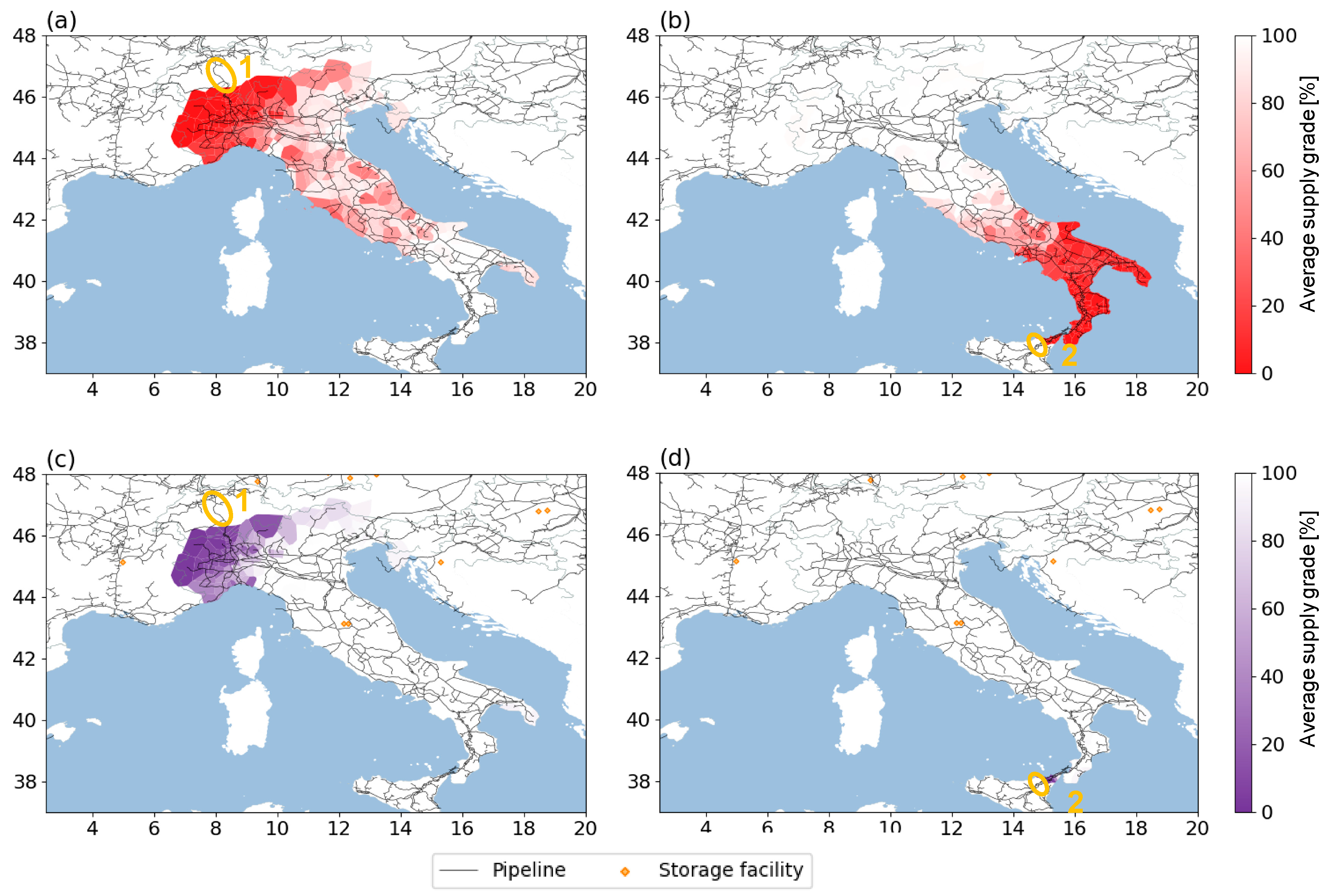
3.2. Supply Grade Mapping

Out of the six pipelines discussed in detail in Section 3.1, two pipelines are further investigated with the supply grade mapping. The two pipelines (Index 1: Trans-Swiss Pipeline and Index 2: Trans-Med Pipeline) are tested with and without storage facilities as the information completeness of storage facilities remains unclear. Those pipelines are neither dead-end pipelines nor existing storage facilities can compensate the related potential outage. This pipeline selection leads, in fact, to a deep dive into the natural gas supply of Italy.
Italy receives natural gas supply from different directions, for example, from the south through Sicily, the Trans-Mediterranean pipeline, or the north through the Passo Gries and the Tarvisio station, besides the numerous LNG terminals [87]. According to the developed model and available information [42], a potential failure of one or both of these pipelines (Index 1: Trans-Swiss Pipeline and Index 2: Trans-Mediterranean pipeline) cannot be fully compensated by the regional available storage facilities. Figure 13a shows the potential failure of the Transitgas pipeline. This outage could cause natural gas shortages spreading over almost all Italian Alpine regions from Liguria along the Alpine chain to Istria in Croatia. While areas of supply shortages decline the more South they are located. The areas with the supply shortages are reduced by consuming from the available natural gas storage facilities (Figure 13), especially in the eastern Alpine region and in Southern Italy.
The potential failure of the pipeline connecting Sicily–Calabria (Trans-Mediterranean pipeline, Figure 13b) could result, in this example, in shortages in southern Italy. The areas with supply shortage are mainly located in Calabria, Basilicata, Puglia, and some parts of Campania. Consuming from natural gas storage facilities (Figure 13d) reduces the areas with supply shortages to the very southwest of Calabria.
Overall, the outcomes of the two potential pipeline failures are mainly driven by the applied flow allocation algorithm that allocates the natural gas flow to the network starting with the closest pipeline and sink (see Section 2.2.2). As the algorithm’s flow allocation is not unique a Monte Carlo simulation was performed. Although a result change below 1% is achieved in all cases with 3500 simulation, 10,000 runs were performed (see SI Section S3: Monte Carlo simulation supply grade mapping) (Supplementary Materials).
It must be noted that the model developed in this study does not consider details of potential packing of pipelines (increase of flow capacities during emergency scenarios). The analysis, however, illustrates that storage facilities can reduce the potential supply loss. Moreover, it also emerges that the storage volumes would need to be able to cover the consumption during the pipeline shutdown.

4. Conclusions

This study illustrates the construction of a complex regional natural gas network model from open-source data and the analysis of potential pipeline disruptions considering seismic and technical hazards. The collection of open-source data to assemble the geospatial European natural gas network is achieved and illustrated. The extensive data collection and processing include information on the natural gas infrastructure components as well as the geographic consumption. A geospatial natural gas infrastructure network model was developed involving pipelines (location and flow capacities), the location of natural gas sources (LNG ports, production platforms and cross-border interconnection points) and the location of natural gas storage facilities.
It is shown that the maximum mean annual technical failure rate of the European natural gas network is up to more than 30 times higher than the mean annual seismic failure rate. The European natural gas network is mainly exposed to seismic hazards in southern and southeastern Europe due to the seismic activities in this region. A common thread of the disruption impact analysis shows that dead-end, sole supply, without storage nearby pipelines are resulting in higher DIM. An exception of this is the high technical and seismic DIM found for the Transitgas pipeline and Trans-Mediterranean pipeline bringing natural gas from the north, respectively from the south to Italy. The results clearly show that storage facilities can reduce the overall disruption impact, e.g., storage facilities can compensate potential flow capacity losses.
For the two mentioned cases (Transitgas pipeline and Trans-Mediterranean pipeline), however, available storage facilities and pipelines cannot fully compensate for a potential failure. Therefore, a supply grade mapping for those two pipelines is conducted and regions in Italy with potential supply shortages are identified making use of a Monte Carlo simulation. The results provide an initial impression and general insights for further analysis, for example, using seasonal variability of natural gas consumption.
Overall, the disruption impact mapping could lead to cost–benefit analysis to support risk-based decision making. It could involve potential fortification of pipelines or installation of storage volumes (pre-event). This is in line with the calls of the United Nations’ Sendai Framework for Disaster Risk Reduction to prevent and reduce the exposure and vulnerability to disasters, increase preparedness for response and recovery and thus strengthen our society [88]. The presented methods could also support future infrastructure planning as resulting from infrastructure projects (e.g., “One Belt One Road” Initiative (一带一路) with the ultimate goal to promote cooperation in the connectivity of energy infrastructure [39].
Since disruptions do happen regardless of the preparation and mitigation strategies, increased attention is given worldwide to the resilience of infrastructure systems. The presented methods could be a possible starting point for a resilience assessment of the European natural gas network with respect to natural (e.g., seismic) and technical hazards. Such an assessment, however, would require not only the disruption analysis, but also extensive and complex simulations of recovery processes to result in a comprehensive resilience assessment.

Supplementary Materials

The following are available online at https://www.mdpi.com/1996-1073/12/24/4685/s1.

Author Contributions

The conceptualization of the paper was done by P.L., F.S., M.S., P.B. and B.S.; M.S., P.B. and B.S. contributed to the model implementation as well as supervision proofreading, discussing results and implications and the editing process. Furthermore, they initiated the research and contributed to writing the text. P.L. managed the reviewing and editing process; P.L. and F.S. developed the models, codes and collected the data; P.L. drafted the paper.

Funding

The research was conducted at the Future Resilient Systems (FRS) at the Singapore-ETH Centre (SEC), which was established collaboratively between ETH Zürich and Singapore’s National Research Foundation (FI 370074011) under its Campus for Research Excellence and Technological Enterprise (CREATE) programme.

Acknowledgments

The natural gas network data stems from the Transparency Platform of ENTSOG and/or its members. Special support was received from Kim Wansub, who was always available for questions regarding coding in Python and MATLAB as well as GIS data processing.

Conflicts of Interest

The authors declare no conflict of interest. The funders had no role in the design of the study; in the collection, analyses, or interpretation of data; in the writing of the manuscript, or in the decision to publish the results.

Abbreviations

APIApplication Programming Interface
DIMDisruption Impact
E-PRTREuropean Pollutant Release and Transfer Register
ENSADEnergy-related Severe Accident Database
ENTSOGEuropean Network of Transmission System Operators for Gas
EGIGEuropean Gas pipeline Incident data Group
ESHM13European Seismic Hazard Model
FRSSeismic hazard failure rate
FRTTechnical failure rate
GISGeographic Information Systems
IEAInternational Energy Agency
LNGLiquefied Natural Gas
OCOther Consumers
PGAPeak Ground Acceleration
PGVPeak Ground Velocity
PGMPeak Ground Motion
PSIPaul Scherrer Institute
SGMSupply grade

References

  1. IEA. World Energy Statistics and Balances; International Energy Agency: Paris, France, 2017. [Google Scholar]
  2. IEA. Outlook for Natural Gas; International Energy Agency (IEA): Paris, France, 2017. [Google Scholar]
  3. Carvalho, R.; Buzna, L.; Bono, F.; Masera, M.; Arrowsmith, D.K.; Helbing, D. Resilience of natural gas networks during conflicts, crises and disruptions. PLoS ONE 2014, 9, e90265. [Google Scholar] [CrossRef] [PubMed] [Green Version]
  4. Austvik, O.G. The energy union and security-of-gas supply. Energy Policy 2016, 96, 372–382. [Google Scholar] [CrossRef]
  5. Tirone, J.; Wabl, M. Austrian gas pipeline explosion disrupts key EU supply hub. In Bloomberg Markets; Bloomberg: New York, NY, USA, 2017. [Google Scholar]
  6. Carvalho, R.; Buzna, L.; Bono, F.; Gutiérrez, E.; Just, W.; Arrowsmith, D. Robustness of trans-European gas networks. Phys. Rev. E 2009, 80, 016106. [Google Scholar] [CrossRef] [PubMed]
  7. Poljansek, K.; Bono, F.; Gutiérrez, E. Seismic risk assessment of interdependent critical infrastructure systems: The case of european gas and electricity networks. Earthq. Eng. Struct. Dyn. 2012, 41, 61–79. [Google Scholar] [CrossRef]
  8. Poljansek, K.; Bono, F.; Gutiérrez, E. Gis-Based Method to Assess Seismic Vulnerability of Interconnected Infrastructure: A Case of EU Gas and Electricity Networks; No. JRC57064; Publications Office of the European Union JRC: Geel, Belgium, 2010. [Google Scholar]
  9. Kaplan, S.; Garrick, B.J. On the quantitative definition of risk. Risk Anal. 1981, 1, 11–27. [Google Scholar] [CrossRef]
  10. Heinimann, H.R. A generic framework for resilience assessment. In Resource Guide on Resilience; EPFL International Risk Governance Center: Lausanne, Switzerland, 2016. [Google Scholar]
  11. Hosseini, S.; Barker, K.; Ramirez-Marquez, J.E. A review of definitions and measures of system resilience. Reliab. Eng. Syst. Saf. 2016, 145, 47–61. [Google Scholar] [CrossRef]
  12. Heinimann, H.R.; Hatfield, K. Infrastructure resilience assessment, management and governance—State and perspectives. In Resilience-Based Approaches to Critical Infrastructure Safeguarding; NATO: Ponta Delgada, Portugal, 2017. [Google Scholar]
  13. Ganin, A.A.; Massaro, E.; Gutfraind, A.; Steen, N.; Keisler, J.M.; Kott, A.; Mangoubi, R.; Linkov, I. Operational resilience: Concepts, design and analysis. Sci. Rep. 2016, 6, 19540. [Google Scholar] [CrossRef] [Green Version]
  14. Didier, M.; Broccardo, M.; Esposito, S.; Stojadinovic, B. A compositional demand/supply framework to quantify the resilience of civil infrastructure systems (Re-CoDeS). Sustain. Resilient Infrastruct. 2017, 3, 86–102. [Google Scholar] [CrossRef] [Green Version]
  15. Gasser, P.; Lustenberger, P.; Cinelli, M.; Kim, W.; Spada, M.; Burgherr, P.; Hirschberg, S.; Stojadinovic, B.; Sun, T.Y. A review on resilience assessment of energy systems. Sustain. Resilient Infrastruct. 2019, 1–27. [Google Scholar] [CrossRef] [Green Version]
  16. Burgherr, P.; Giroux, J.; Spada, M. Accidents in the energy sector and energy infrastructure attacks in the context of energy security. Eur. J. Risk Regul. 2015, 6, 271–283. [Google Scholar] [CrossRef]
  17. Blaikie, P.; Cannon, T.; Davis, I.; Wisner, B. At Risk: Natural hazards, People’s Vulnerability and Disasters; Routledge: Abingdon, UK, 2004. [Google Scholar]
  18. HAZUS. Multi-Hazard Loss Estimation Methodology—Hurricane Model; FEMA: Washington, DC, USA, 2003.
  19. HAZUS. Multi-Hazard Loss Estimation Methodology—Earthquake Model; FEMA: Washington, DC, USA, 2003.
  20. HAZUS. Multi-Hazard Loss Estimation Methodology—Flood Model; FEMA: Washington, DC, USA, 2003.
  21. GEM. Gem Physical Vulnerability Functions Database. 2016. Available online: https://www.globalquakemodel.org (accessed on 9 December 2019).
  22. Hirschberg, S.; Spiekerman, G.; Dones, R. Severe Accidents in the Energy Sector; Paul Scherrer Institut, Villigen PSI: Villigen, Switzerland, 1998; p. 340. [Google Scholar]
  23. Kim, W.; Burgherr, P.; Spada, M.; Lustenberger, P.; Kalinina, A.; Hirschberg, S. Energy-related severe accident database (ensad): Cloud-based geospatial platform. Big Earth Data 2019, 2, 368–394. [Google Scholar] [CrossRef] [Green Version]
  24. Gao, J.; Liu, X.; Li, D.; Havlin, S. Recent progress on the resilience of complex networks. Energies 2015, 8, 12187–12210. [Google Scholar] [CrossRef] [Green Version]
  25. Mieler, M.; Stojadinovic, B.; Budnitz, R.; Comerio, M.; Mahin, S. A framework for linking community-resilience goals to specific performance targets for the built environment. Earthq. Spectra 2015, 8, 12187–12210. [Google Scholar] [CrossRef] [Green Version]
  26. Helbing, D. Globally networked risks and how to respond. Nature 2013, 497, 51–59. [Google Scholar] [CrossRef]
  27. Voropai, N.I.; Senderov, S.M.; Edelev, A.V. Detection of “bottlenecks” and ways to overcome emergency situations in gas transportation networks on the example of the European gas pipeline network. Energy 2012, 42, 3–9. [Google Scholar] [CrossRef]
  28. Yu, W.; Song, S.; Li, Y.; Min, Y.; Huang, W.; Wen, K.; Gong, J. Gas supply reliability assessment of natural gas transmission pipeline systems. Energy 2018, 162, 853–870. [Google Scholar] [CrossRef]
  29. Gjorgiev, B.; Antenucci, A.; Volkanovski, A.; Sansavini, G. An FTA method for the unavailability of supply in gas networks supported by physical models. IEEE Trans. Reliab. 2019. [Google Scholar] [CrossRef]
  30. Su, H.; Zhang, J.; Zio, E.; Yang, N.; Li, X.; Zhang, Z. An integrated systemic method for supply reliability assessment of natural gas pipeline networks. Appl. Energy 2018, 209, 489–501. [Google Scholar] [CrossRef]
  31. Praks, P.; Kopustinskas, V.; Masera, M. Monte-carlo-based reliability and vulnerability assessment of a natural gas transmission system due to random network component failures. Sustain. Resilient Infrastruct. 2017, 2, 97–107. [Google Scholar] [CrossRef]
  32. Kopustinskas, V.; Praks, P. Probabilistic gas transmission network simulator and application to the EU gas transmission system. In Summer Safety & Reliability Seminars SSARS 2015; SSARS: Gdańsk/Sopot, Poland, 2015. [Google Scholar]
  33. Praks, P.; Kopustinskas, V.; Masera, M. Probabilistic modelling of security of supply in gas networks and evaluation of new infrastructure. Reliab. Eng. Syst. Saf. 2015, 144, 254–264. [Google Scholar] [CrossRef]
  34. Sacco, T.; Compare, M.; Zio, E.; Sansavini, G. Portfolio decision analysis for risk-based maintenance of gas networks. J. Loss Prev. Process Ind. 2019, 60, 269–281. [Google Scholar] [CrossRef]
  35. Hauser, P.; Hobbie, H.; Möst, D. Resilience in the German natural gas network: Modelling approach for a high-resolution natural gas system. In Proceedings of the 2017 14th International Conference on the European Energy Market (EEM), Dresden, Germany, 6–9 June 2017. [Google Scholar]
  36. Hauser, P.; Heidari, S.; Weber, C.; Möst, D. Does increasing natural gas demand in the power sector pose a threat of congestion to the german gas grid? A model-coupling approach. Energies 2019, 1, 2159. [Google Scholar] [CrossRef] [Green Version]
  37. Jensen, T.V.; Pinson, P. Re-europe, a large-scale dataset for modeling a highly renewable European electricity system. Sci. Data 2017, 4, 170175. [Google Scholar] [CrossRef] [PubMed] [Green Version]
  38. Pfenninger, S.; DeCarolis, J.; Hirth, L.; Quoilin, S.; Staffell, I. The importance of open data and software: Is energy research lagging behind? Energy Policy 2017, 101, 211–215. [Google Scholar] [CrossRef]
  39. Swiss, Re. China’s Belt & Road Initiative: The Impact on Commercial Insurance in Participating Regions. In Sigma; Swiss Re: Zurich, Switzerland, 2017. [Google Scholar]
  40. Spada, M.; Burgherr, P. A hierarchical approximate bayesian computation (habc) for accident risk in the energy sector triggered by natural events. In Proceedings of the European Safety and Reliability Conference (ESREL), Hannover, Germany, 22–26 September 2019. [Google Scholar]
  41. Lustenberger, P.; Kim, W.; Schumacher, F.; Spada, M.; Burgherr, P.; Hirschberg, S.; Stojadinovic, B. Network analysis of the European natural gas infrastructure to quantify its performance in long-term pipeline shutdown scenarios. In Proceedings of the European Safety and Reliability Conference (ESREL), Trondheim, Norway, 17–21 June 2018. [Google Scholar]
  42. ENTSOG. Entsog Transparancy Platform. 2016. Available online: http://www.entsog.eu/ (accessed on 15 October 2017).
  43. El-Shiekh, T. The optimal design of natural gas transmission pipelines. Energy Sources Part B Econ. Plan. Policy 2013, 8, 7–13. [Google Scholar] [CrossRef]
  44. Martin, A.; Möller, M.; Moritz, S. Mixed integer models for the stationary case of gas network optimization. Math. Program. 2005, 105, 563–582. [Google Scholar] [CrossRef]
  45. Perner, J. Die Langfristige Erdgasversorgung Europas: Analysen und Simulationen Mit dem Angebotsmodell Eugas; Zeitschrift für Energiewirtschaft, Springer: Berlin, Germany, 2002. [Google Scholar]
  46. IEA. North American Energy Industrial Complex—Pipelines; IEA: Paris, France, 2017. [Google Scholar]
  47. FNB. Transmission System—Facts and Figures; FNB: Pittsburgh, PA, USA, 2017; Available online: http://www.fnb-gas.de/en/transmission-systems/facts-and-figures/facts-and-figures.html (accessed on 15 October 2017).
  48. Zhao, Y.; Rui, Z. Pipeline compressor station construction cost analysis. Int. J. Oil Gas Coal Technol. 2014, 8, 41–61. [Google Scholar] [CrossRef]
  49. Messersmith, D.; Brockett, D.; Loveland, D. Understanding Natural Gas Compressor Stations. 2015. Available online: https://extension.psu.edu/downloadable/download/sample/sample_id/755/ (accessed on 15 October 2017).
  50. QGIS Development Team. Qgis Geographic Information System 2.18; QGIS Development Team: ’s-Hertogenbosch, The Netherlands, 2016. [Google Scholar]
  51. BP. Statistical Review of World Energy; BP: London, UK, 2018. [Google Scholar]
  52. Enipedia. 2017. Available online: http://enipedia.tudelft.nl/wiki/Main_Page (accessed on 1 July 2017).
  53. GlobalEnergyObservatory. 2017. Available online: http://www.globalenergyobservatory.com/ (accessed on 1 July 2017).
  54. European Environment Agency (EEA). European Pollutant Release and Transfer Register (E-Prtr); European Environment Agency: København, Denmark, 2017; Available online: https://prtr.eea.europa.eu/-/home (accessed on 1 July 2017).
  55. Center for International Earth Science Information Network—CIESIN—Columbia University. Gridded Population of the World, Version 4 (gpwv4): Population Count Adjusted to Match 2015 Revision of Un Wpp Country Totals, Revision 10; NASA Socioeconomic Data and Applications Center (SEDAC): Palisades, NY, USA, 2017. [Google Scholar]
  56. GADM. Gadm Database of Global Administrative Areas (v3.6). 2017. Available online: http://www.gadm.org/ (accessed on 15 October 2017).
  57. Woessner, J.; Laurentiu, D.; Giardini, D.; Crowley, H.; Cotton, F.; Grünthal, G.; Valensise, G.; Arvidsson, R.; Basili, R.; Demircioglu, M.B.; et al. The 2013 European seismic hazard model: Key components and results. Bull. Earthq. Eng. 2015, 13, 3553–3596. [Google Scholar] [CrossRef] [Green Version]
  58. CEN. Eurocode 8: Design of Structures for Earthquake Resistance, in Part 1: General Rules, Seismic Actions and Rules for Buildings; CEN: Brussels, Belgium, 2004. [Google Scholar]
  59. Burgherr, P.; Hirschberg, S. Comparative risk assessment of severe accidents in the energy sector. Energy Policy 2014, 74, S45–S56. [Google Scholar] [CrossRef]
  60. Felder, F. A critical assessment of energy accident studies. Energy Policy 2009, 37, 5744–5751. [Google Scholar] [CrossRef]
  61. Burgherr, P.; Spada, M.; Kalinina, A.; Hirschberg, S.; Kim, W.; Gasser, P.; Lustenberger, P. The Energy-Related Severe Accident Database (ENSAD) for Comparative Risk Assessment of Accidents in the Energy Sector. In European Safety and Reliability Conference (ESREL); CRC Press, Taylor & Francis Group: London, UK, 2017. [Google Scholar]
  62. Henry, D.; Ramirez-Marquez, J.E. Generic metrics and quantitative approaches for system resilience as a function of time. Reliab. Eng. Syst. Saf. 2012, 99, 114–122. [Google Scholar] [CrossRef]
  63. Nan, C.; Sansavini, G.; Kröger, W. Building an Integrated Metric for Quantifying the Resilience of Interdependent Infrastructure Systems; Springer: Cham, Switzerland, 2015. [Google Scholar]
  64. Kyriakidis, M.; Lustenberger, P.; Burgherr, P.; Dang, V.N.; Hirschberg, S. Quantifying energy systems resilience—A simulation approach to assess recovery. Energy Technol. 2018, 6, 1700–1706. [Google Scholar] [CrossRef]
  65. Eurogas. Eurogas Statisitcal Report 2016; Eurogas: Bruxelles, Belgium, 2016. [Google Scholar]
  66. Pustišek, A.; Karasz, M. Natural Gas: A Commercial Perspective; Springer: Berlin/Heidelberg, Germany, 2017. [Google Scholar]
  67. Moran, M.J.; Shapiro, H.N.; Boettner, D.D.; Bailey, M.B. Fundamentals of Engineering Thermodynamics; John Wiley & Sons: Hoboken, NJ, USA, 2010. [Google Scholar]
  68. Eurostat. Simplified Energy Balances—Annual Data; Eurostat: Bruxelles, Belgium, 2018. [Google Scholar]
  69. Aurenhammer, F. Voronoi diagrams—A survey of a fundamental geometric data structure. ACM Comput. Surv. (CSUR) 1991, 23, 345–405. [Google Scholar] [CrossRef]
  70. Lustenberger, P.; Sun, T.; Gasser, P.; Kim, W.; Spada, M.; Burgherr, P.; Hirschberg, S.; Stojadinović, B. Potential Impacts of Selected Natural Hazards and Technical Failures on the Natural Gas Tranmission Network in Europe, in European SAFETY and Reliability Conference (ESREL); Taylor & Francis: Portoroz, Slovenia, 2017. [Google Scholar]
  71. Ford, L.; Fulkerson, D. Maximal flow through a network. Can. J. Math. 1956. [Google Scholar] [CrossRef]
  72. Boykov, Y.; Kolmogorov, V. An experimental comparison of min-cut/max-flow algorithms for energy minimization in vision. IEEE Trans. Pattern Anal. Mach. Intell. 2004, 26, 1124–1137. [Google Scholar] [CrossRef] [Green Version]
  73. MATLAB. Versin r2015b; The MathWorks Inc.: Natick, MA, USA, 2015. [Google Scholar]
  74. Csardi, G.; Nepusz, T. The igraph software package for complex network research. InterJournal Complex Syst. 2006, 1695, 1–9. [Google Scholar]
  75. Caprio, M.; Tarigan, B.; Worden, C.B.; Wiemer, S.; Wald, D.J. Ground motion to intensity conversion equations (gmices): A global relationship and evaluation of regional dependency. Bull. Seismol. Soc. Am. 2015, 105, 1476–1490. [Google Scholar] [CrossRef]
  76. EGIG. 9th Report of the European Gas Pipeline Incident Data Group (Period 1970–2013); EGIG: Groningen, The Netherlands, 2015. [Google Scholar]
  77. Nicholson, C.D.; Barker, K.; Ramirez-Marquez, J.E. Flow-based vulnerability measures for network component importance: Experimentation with preparedness planning. Reliab. Eng. Syst. Saf. 2016, 145, 62–73. [Google Scholar] [CrossRef]
  78. Docker Inc. Docker; Docker Inc.: San Francisco, CA, USA, 2019. [Google Scholar]
  79. Grünthal, G.; Wahlström, R. The European-mediterranean earthquake catalogue (EMEC) for the last millennium. J. Seismol. 2012, 16, 535–570. [Google Scholar] [CrossRef] [Green Version]
  80. Transitgas. The Pipeline System. 2017. Available online: http://www.transitgas.org/EN/ (accessed on 15 October 2017).
  81. Transmed. Gas Transportation System. 2017. Available online: http://www.transmed-spa.it/?lingua=2 (accessed on 10 October 2017).
  82. GreenStream. The Greenstream Pipeline. 2017. Available online: http://www.greenstreambv.com/en/pages/home.shtml (accessed on 10 October 2017).
  83. ETNSOG. Union-Wide Simulation of Gas Supply and Infrastructure Disruption Scenarios (SOS Simulation); ENTSOG: Bruxelles, Belgium, 2017. [Google Scholar]
  84. TANAP. Trans Anatolian Natural Gas Pipeline Project. 2017. Available online: http://www.tanap.com/ (accessed on 10 October 2017).
  85. AdriaticLNG. Cavarzere Porto Levante. 2017. Available online: http://www.adriaticlng.it/en/home/ (accessed on 10 October 2017).
  86. Tsionis, G.; Pinto, A.; Giardini, D.; Mignan, A.; Cotton, F.; Danciu, L.; Iervolino, I.; Pitilakis, K.; Stojadinovic, B.; Zwicky, P. Harmonized Approach to Stress Tests for Critical Infrastructures Against Natural Hazards; Joint Research Centre (JRC): Luxembourg, 2016. [Google Scholar]
  87. Vainio, J. An Explosion in the Heart of the European Gas System: What does the Baumgarten Case Tell about the Resiliency of the System? 2017. Available online: https://www.enseccoe.org/data/public/uploads/2017/12/sardines-2017_512_baumgarten-explosion-and-gas-system-resiliency-in-europe.pdf (accessed on 20 January 2018).
  88. UN General Assembly. The Sendai Framework for Disaster Risk Reduction; UN General Assembly: New York, NY, USA, 2015; pp. 2015–2030. [Google Scholar]
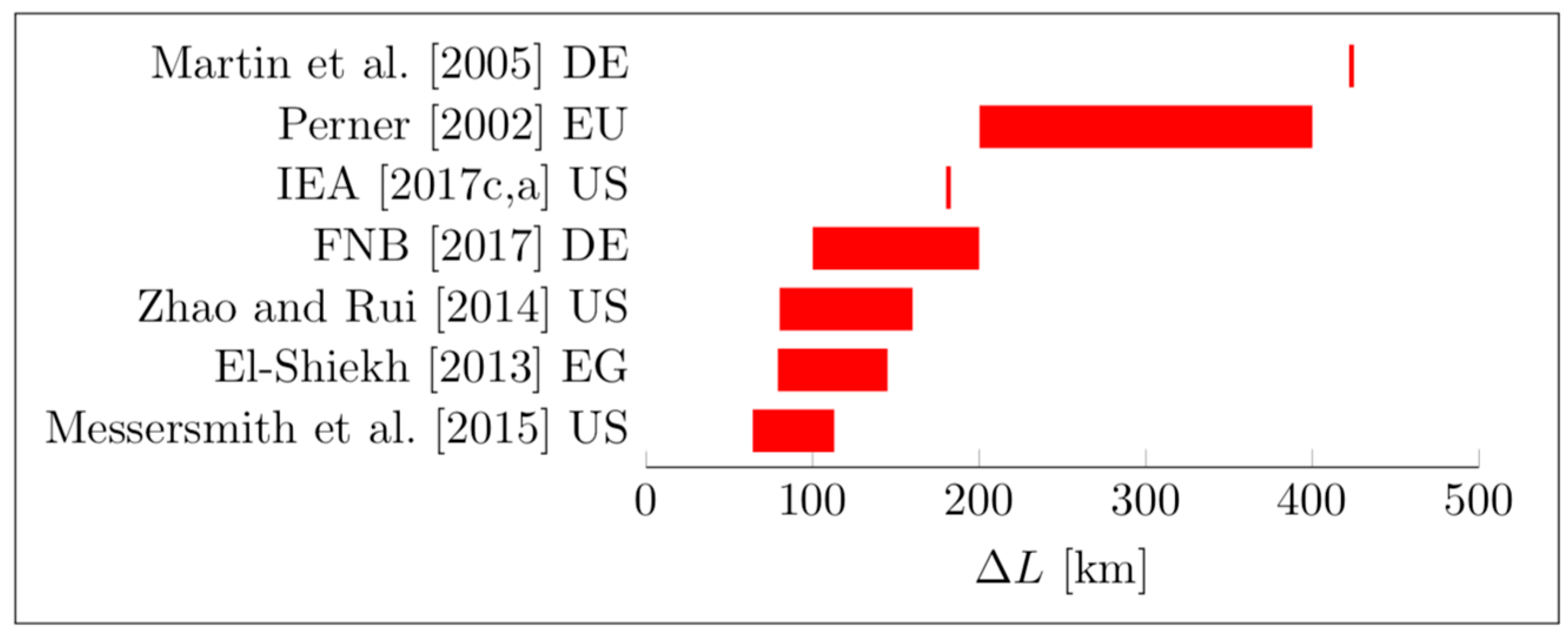
Figure 1. Downloaded European Network of Transmission System Operators for Gas (ENTSOG) pipeline maps. Each map consists of 1024 tile maps (raster grid).
Energies 12 04685 g001
Figure 2. Image and data processing from the tile maps (high resolution images) to the pipeline shapefile.
Energies 12 04685 g002
Figure 3. Average distance ΔL between compressor stations with corresponding source and country.
Energies 12 04685 g003
Figure 4. Graphical representation of the natural gas infrastructure network. Displayed are the pipelines, identified sources and the storage facilities.
Energies 12 04685 g004
Figure 5. Schematic overview of the natural gas network analysis. The component failure rate can be represented by the mean annual seismic failure rate seismic hazard failure rate (FRs) or the mean annual technical failure rate technical failure rate (FRT).
Energies 12 04685 g005
Figure 6. Flow chart to illustrate the allocation of natural gas consumption to the identified sinks. The allocation is done in two steps. In Step 1 (left side), the natural gas consumption is geographically mapped. In Step 2 (right side), the consumption is assigned to the natural gas network.
Energies 12 04685 g006
Figure 7. Spatial distribution of other consumers (OC) of natural gas.
Energies 12 04685 g007
Figure 8. Conceptual illustration of the transformation of a multiple source/sink problem to a single source/sink problem.
Energies 12 04685 g008
Figure 9. European seismic hazard map for peak ground acceleration (PGA) values with a 10% probability of exceedance in a 50 years period in units of standard gravity (g) [57].
Energies 12 04685 g009
Figure 10. Seismic hazard analysis for natural gas pipelines with the infrastructure data and the seismic hazard map [57].
Energies 12 04685 g010
Figure 11. Disruption impact (DIM) of seismic hazards without storage facilities for Europe (a) and with storage facilities for Europe (b) using an average compressor stations distance of 64 km. The labels 1–3 represent the pipelines with the highest system performance loss (ΔFmax,i) combined with seismic hazard exposure.
Energies 12 04685 g011aEnergies 12 04685 g011b
Figure 12. Disruption impact related to technical hazards without storage facilities for Europe (a) and with storage facilities for Europe (b). The index 1–6 is representing the six pipelines with the highest system performance loss (ΔFmax,i).
Energies 12 04685 g012aEnergies 12 04685 g012b
Figure 13. Monte Carlo Simulation (10,000 runs) mapping of the average supply grade coverage for a potential failure of the Transitgas pipeline (Passo Gries, Index 1) without storage facilities (a) and with storage facilities (c). Mapping of the supply grade coverage for a potential failure of the Trans-Mediterranean pipeline (Sicily–Calabria pipeline, Index 2) without storage facilities (b) and with storage facilities (d). The yellow circle indicates the pipeline taken out for the simulation.
Energies 12 04685 g013
Table 1. Overview of natural gas network disruption analysis literature.
StudyMethodologiesCase Study
Topological AnalysisThermal-Hydraulic Flow ComputationEconomic ModelsStochastic Failure EstimationEuropeGreat BritainGermany“Fictitious” Real World Network
Carvalho et al., 2009 [6]XX X
Carvalho et al., 2014 [3] X X
Gjorgiev et al., 2019 [29] X X X
Hauser et al., 2017 [35] X X
Hauser et al., 2019 [36] X X
Kopustinskas and Praks 2015 [32] X X
Poljansek et al., 2012 [7]X XX
Praks et al., 2017 [31] X X
Praks et al., 2015 [33] X X
Sacco et al., 2019 [34] XX X
Su et al., 2018 [30] XXX X
Voropai et al., 2012 [27] X X
Yu et al., 2018 [28] XX X
Table 2. Geospatial infrastructure data collected, processed and employed for the present analysis.
DatasetTypeSourceDescription
Natural gas pipelinesShapefile
(Polyline)
ENTSOG 2016 [42]European natural gas pipelines categorized in three diameter classes (8157 pipelines, 197,612 km)
Natural gas storage facilitiesShapefile
(Points)
ENTSOG 2016 [42]European natural gas storage facilities with location, facility name and storage volume (152 entries)
Natural gas sourcesShapefile
(Points)
ENTSOG 2016 [42]European natural gas sources (LNG ports, production platforms and cross-border interconnection points)
Table 3. Categorized pipelines according to the diameter and related average flow capacity from Carvalho et al., 2009 [6]. The upper limit was used for model development.
Pipeline Diameter CategoryDiameter d (inch)Capacity C (109 m3/yr)
Small pipelinesd ≤ 24C < 3.942
Medium pipelines24 < d ≤ 363.942 ≤ C < 8.76
Large pipelines36 < d8.76 ≤ C < 87.6
Table 4. Data for the geographic natural gas consumption allocation.
DatasetTypeSourceDescription
Population countGeotiff, Raster (30 arc-seconds)Center for International Earth Science Information Network -CIESIN-Columbia University 2017 [55]The population count per pixel from UN WPP-Adjusted Population Count, v4.10 (2015)
Country boundariesShapefile (Polygon)GADM 2017 [56]Worldwide country boundaries (administrative level 0)
Natural gas power plantsShapefile
(Points)
Enipedia [52]European natural gas power plants with associated annual carbon dioxide emissions (565 with complete information)
National natural gas consumptionTableIEA 2017 [1]Annual natural gas production, imports and exports on country level (reference year 2015)
Table 5. Parameters for the ground motion to intensity conversion in Equation Equations (12) and (13) [75].
PGMα1α2β1β2tPGM
PGA2.270−1.3611.6473.8221.6
PGV4.4244.0181.5892.6710.3
Table 6. Estimated system performance losses ΔFmax,i, without storage facilities for the six pipelines (labeled 1 to 6).
Pipeline IndexΔFmax,i (%)
14.6
23.5
31.8
41.8
51.8
61.1
Table 7. Comparison of seismic and technical failures and disruption impact (without storage facilities).
SeismicTechnical
minmaxmeanstdminmaxmeanstd
Maximum pipeline failure rate (10–3/year)020.10.250770.941.69
Maximum disruption impact (10–4%/year)034.50.070.6901180.443.26

