Classification and Evaluation of Concepts for Improving the Performance of Applied Energy System Optimization Models


Abstract
1. Introduction
1.1. Motivation
1.2. Energy System Optimization Models: Characteristics and Dimensions
1.3. Challenges: Linking Variables and Constraints
2. State of Research
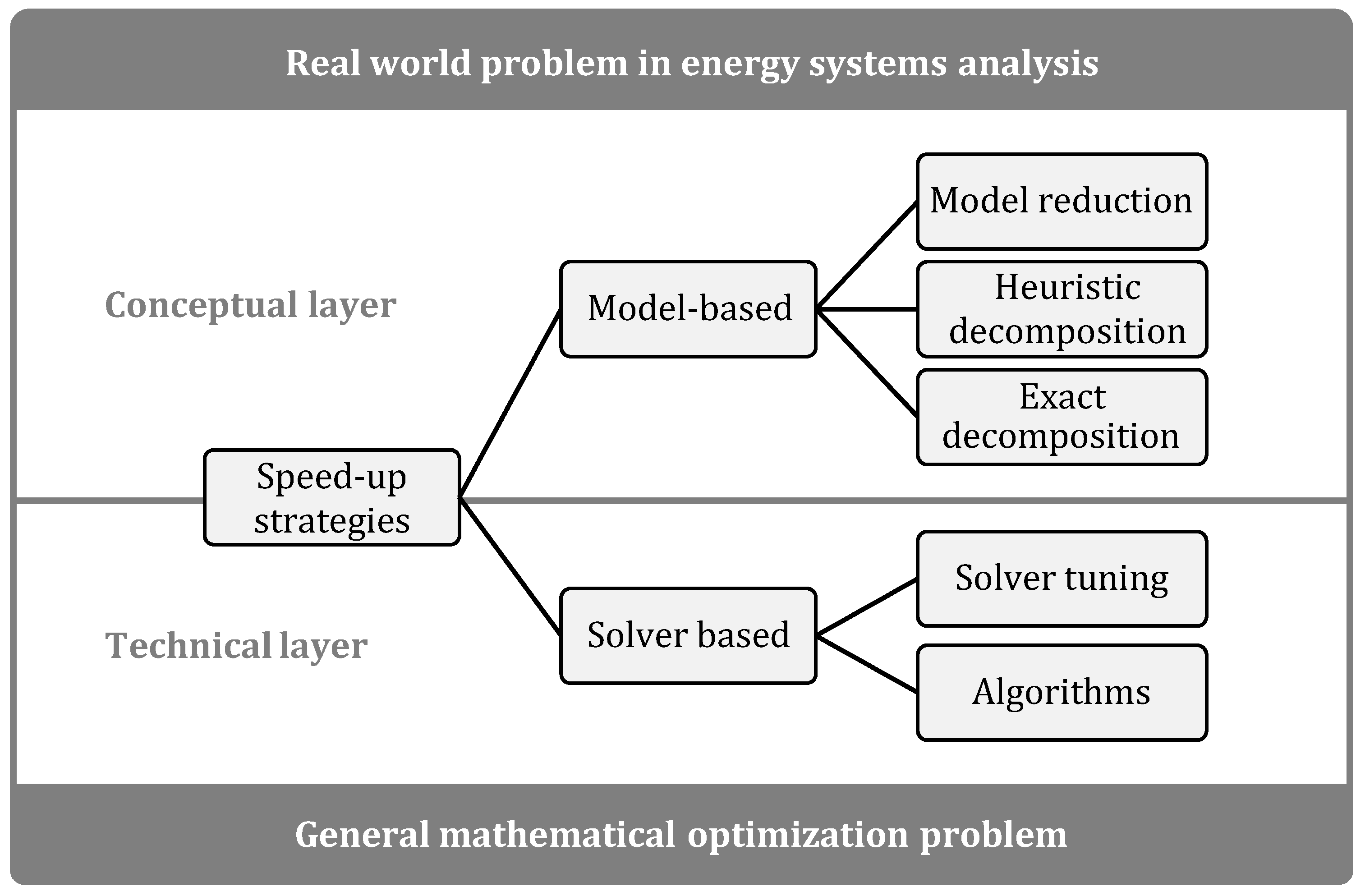
2.1. Classification of Performance Enhancement Approaches
2.2. Model Reduction
2.2.1. Slicing
2.2.2. Spatial Aggregation
2.2.3. Temporal Aggregation
2.2.4. Technological Aggregation
2.3. Heuristic Decomposition and Nested Approaches
2.3.1. Rolling Horizon
2.3.2. Temporal Zooming
2.4. Mathematically Exact Decomposition Techniques
2.4.1. Dantzig-Wolfe Decomposition
2.4.2. Lagrangian Relaxation
2.4.3. Benders Decomposition
2.4.4. Further Aspects
2.5. Aim and Scope
- (1)
- To be able to increase the descriptive complexity of the models, the mathematical complexity is often simplified. This frequently means the formulation of large monolithic linear programs (LPs) which are solved on shared memory machines.
- (2)
- Due to the assessment of high shares of power generation from vRES the time set that represents the sub-annual time horizon shows the largest size (typically 8760 time steps)
- (3)
- A great number of applied ESOMs are based on mathematical programming languages such as GAMS (General Algebraic Modeling System) or AMPL (A Mathematical Programming Language”) rather than on classical programming languages. Those languages enable model formulations which are close to the mathematical problem description and take the task of translation into a format that is readable for solver software. For this reason, the execution time of the appropriate ESOMs can by roughly divided into two parts, the compilation and generation of the model structure requested by the solver and the solver time.
- (1)
- We focus on very large LPs that have a sufficiently large size for the computing time to be dominated by the solver time and still maintaining the possibility to be solved on a single shared memory computer. If we implement an approach that allows for reduction or parallelization of the initial ESOM by treating a particular dimension, the highest potential therefore can explored by applying such an approach to the largest dimension. Accordingly:
- (2)
- We emphasize speed-up strategies that treat the temporal scale of an ESOM. A high potential for performance enhancement still lies in parallelization, even though, for this study, it is limited to parallel threads on shared memory architectures. Exact decomposition techniques have the advantage to enable parallel solving of sub-problems. However, we claim that each exact decomposition technique can be replaced by a heuristic where the iterative solution algorithm is terminated early. In this way, the highest possible performance should be explored, because further iterations only improve the model accuracy; however they require more resources in terms of computing time. In addition, according to the literature in Table 2, it can be concluded, that mathematically exact decomposition techniques are applied less often with the objective of parallel model execution, but the separation of a more complicated optimization problem from an easy-to-solve one. For very large LPs this is not necessary. For these reasons:
- (3)
- We only analyze model reduction by aggregation and heuristic decomposition approaches.
3. Materials and Methods
3.1. Overview
- model reduction by spatial and temporal aggregation
- rolling horizon
- temporal zooming
3.2. Modeling Setup
3.2.1. Characteristic Constraints
3.2.2. Solver Parametrization and Hardware Environment
- (1)
- LP-method: barrier
- (2)
- Cross-Over: disabled
- (3)
- Multi-threading: enabled (16 if not otherwise stated)
- (4)
- Barrier tolerance (barepcomp)
- 1e−5 spatial aggregation with capacity expansion
- default (1e−8): rest
- (5)
- Automatic passing of the presolved dual LP to the solver (predual): disabled
- (6)
- Aggressive scaling (scaind): enabled
3.2.3. Original REMix Instances and Their Size
3.3. Implementations
3.3.1. Aggregation Approaches
3.3.2. Rolling Horizon Dispatch
- (1)
- A new set that represents the time intervals is defined.
- (2)
- The number of overlapping time steps between two intervals as well as a map that assigns the time steps t to the corresponding intervals (with or without overlap) is defined. With a larger overlap more subsequent time steps are redundantly assigned to both the end of the and the beginning of the interval.
- (3)
- It must be ensured that all time dependent elements (variables and constraints) are declared over the whole set of time steps, whereas their definitions are limited to a subset of time steps that depends on the current time interval.
- (4)
- A surrounding loop is added that iterates over the time intervals.
- (5)
- With each iteration a solve statement is executed.
- (6)
- The values of all time dependent variables are fixed for all time steps of the current interval but not for those that belong to the overlap.
- (7)
- To easily obtain the objective value of the full-time horizon model, a final solve is executed that considers only cost relevant equations. As all variable levels are already fixed at this stage, this final solve is not costly in terms of performance.
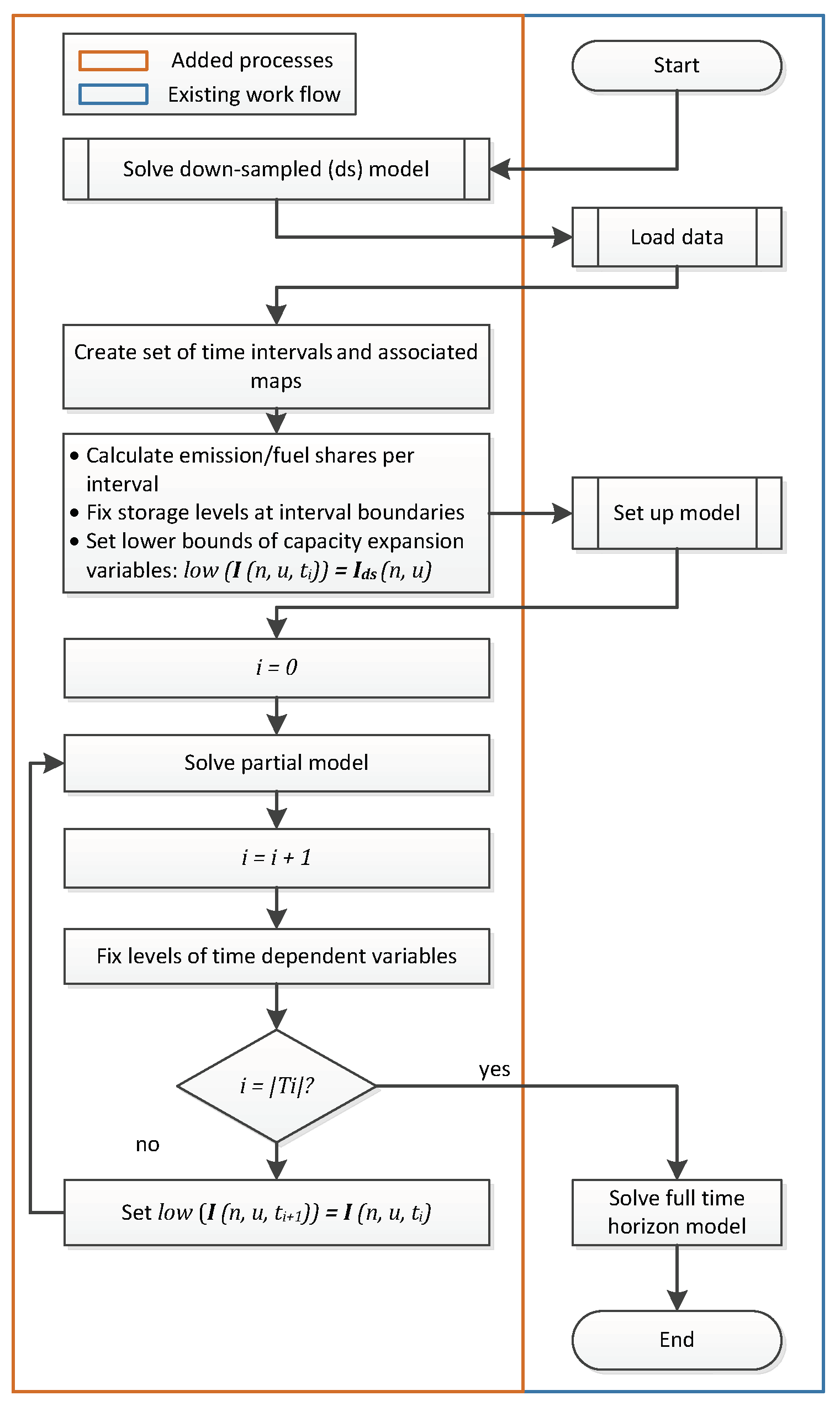
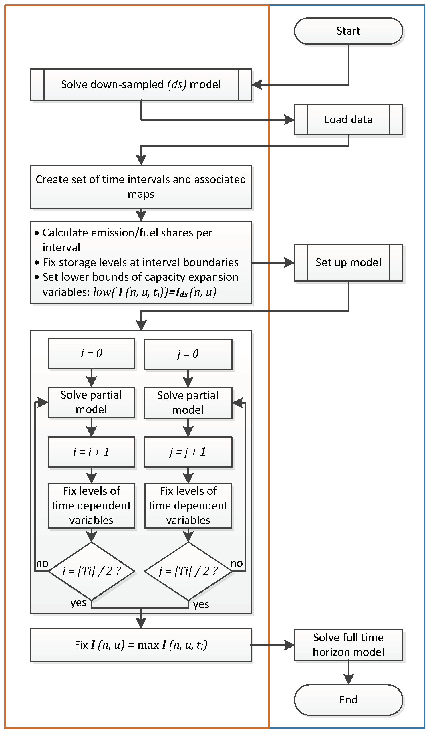
3.3.3. Sub-annual Temporal Zooming
- (1)
- A sequential version that is executed in the same chronological manner as the rolling horizon approach where parallelization only takes place on the solve side (Figure 4).
- (2)
- A parallel version that uses the grid computing facility of GAMS where a defined number of time intervals is solved in parallel. Parallelization takes place on both the model side and the solver side (Figure 5).
3.4. Evaluation Framework
3.4.1. Parameterization of Speed-Up Approaches
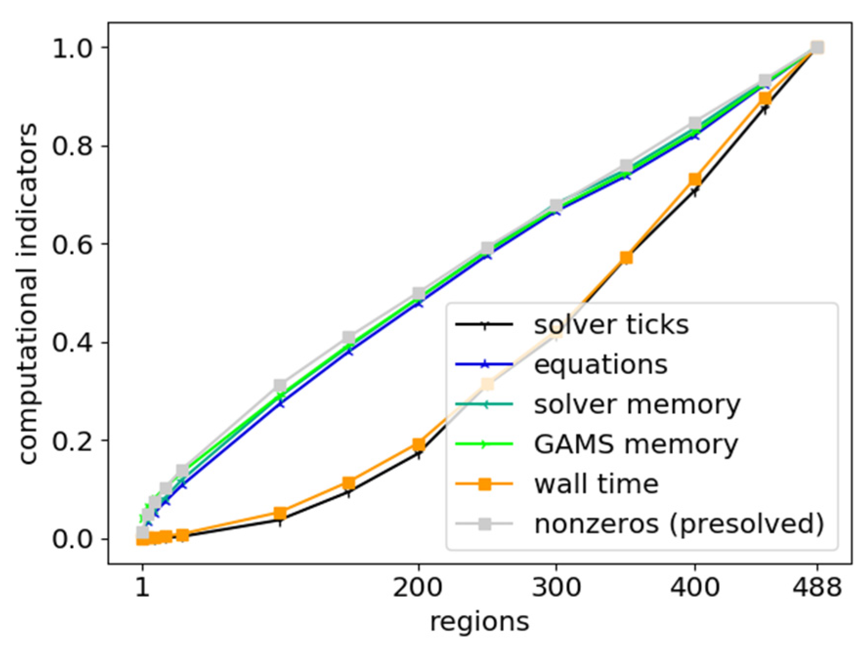
3.4.2. Computational Indicators
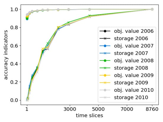
3.4.3. Accuracy Indicators
- (1)
- The “objective value” of the optimization problem.
- (2)
- The technology specific, temporally and spatially summed, annual “power supply” of generators, storage and electricity transmission.
- (3)
- The spatially summed values of “added capacity” for storage and electricity transmission, and
- (4)
- The temporally resolved, but spatially summed “storage levels” of certain technologies.
4. Results
4.1. Pre-analyses and Qualitative Findings
4.1.1. Order of Sets
4.1.2. Sparse vs. Dense
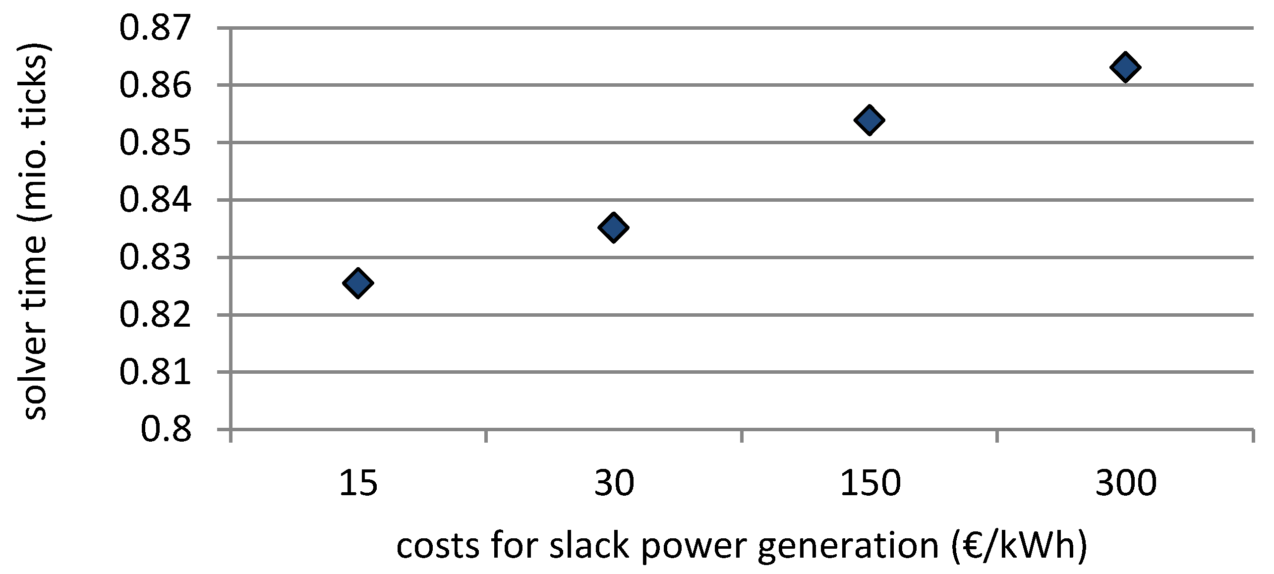
4.1.3. Slack Variables and Punishment Costs
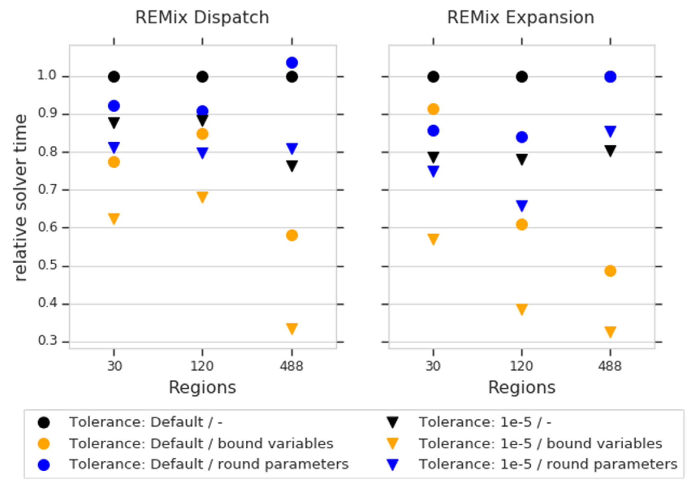
4.1.4. Coefficient Scaling and Variable Bounds
4.2. Aggregation of Individual Dimensions
4.2.1. Spatial
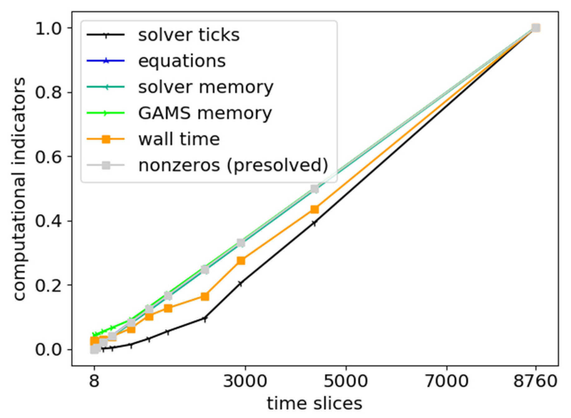
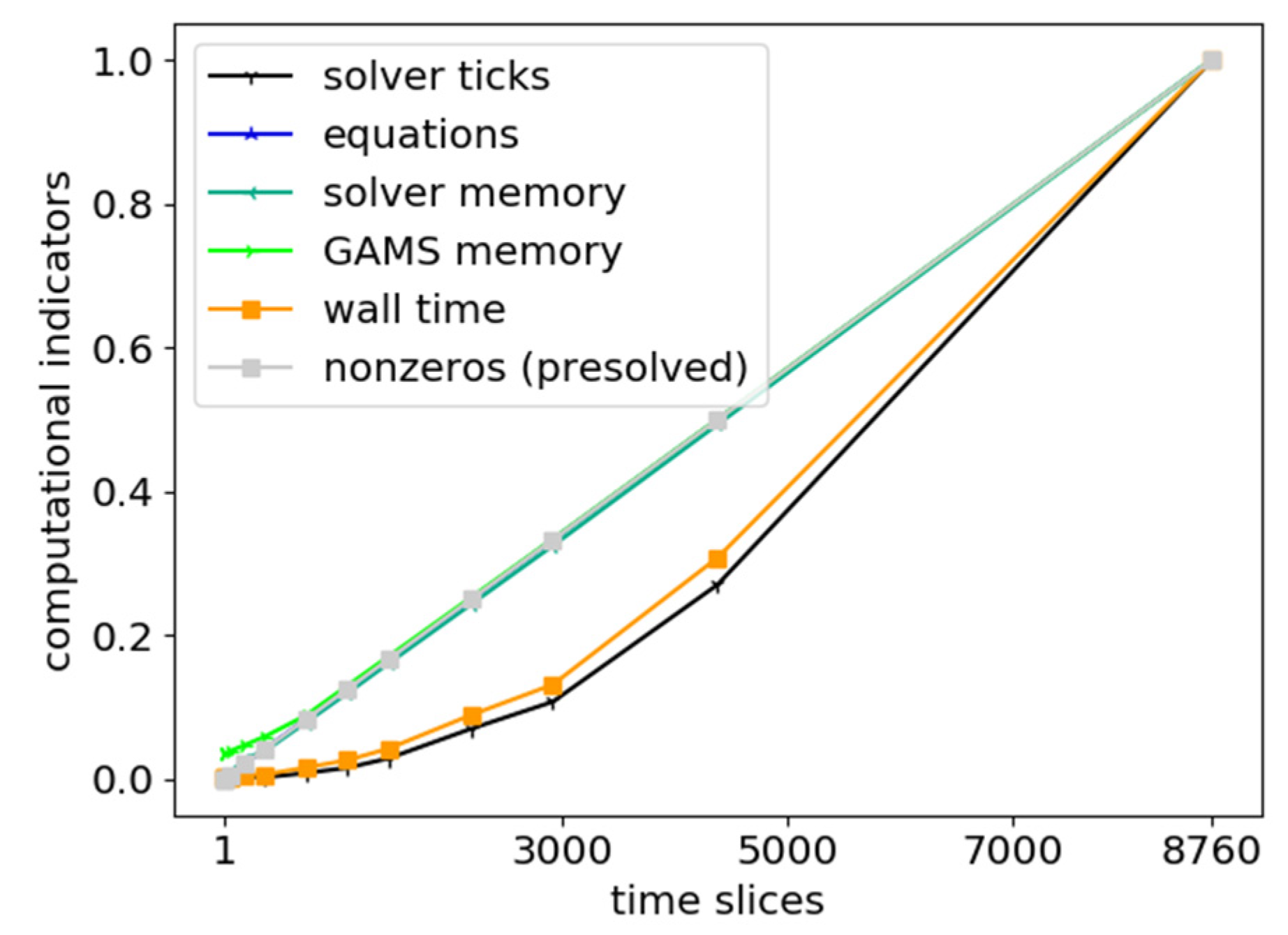
4.2.2. Temporal
4.3. Heuristic Decomposition
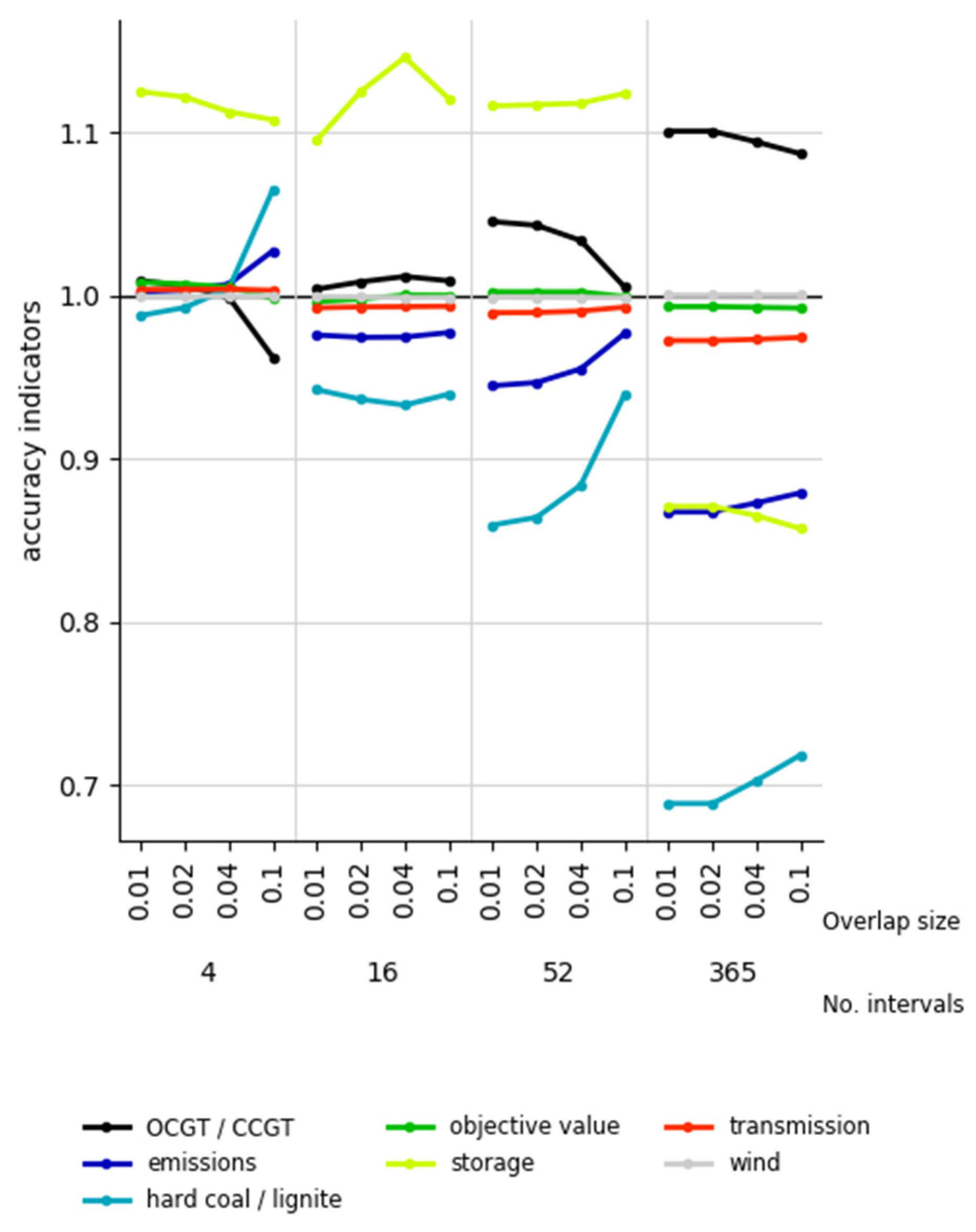
4.3.1. Rolling Horizon Dispatch?
4.3.2. Temporal Zooming
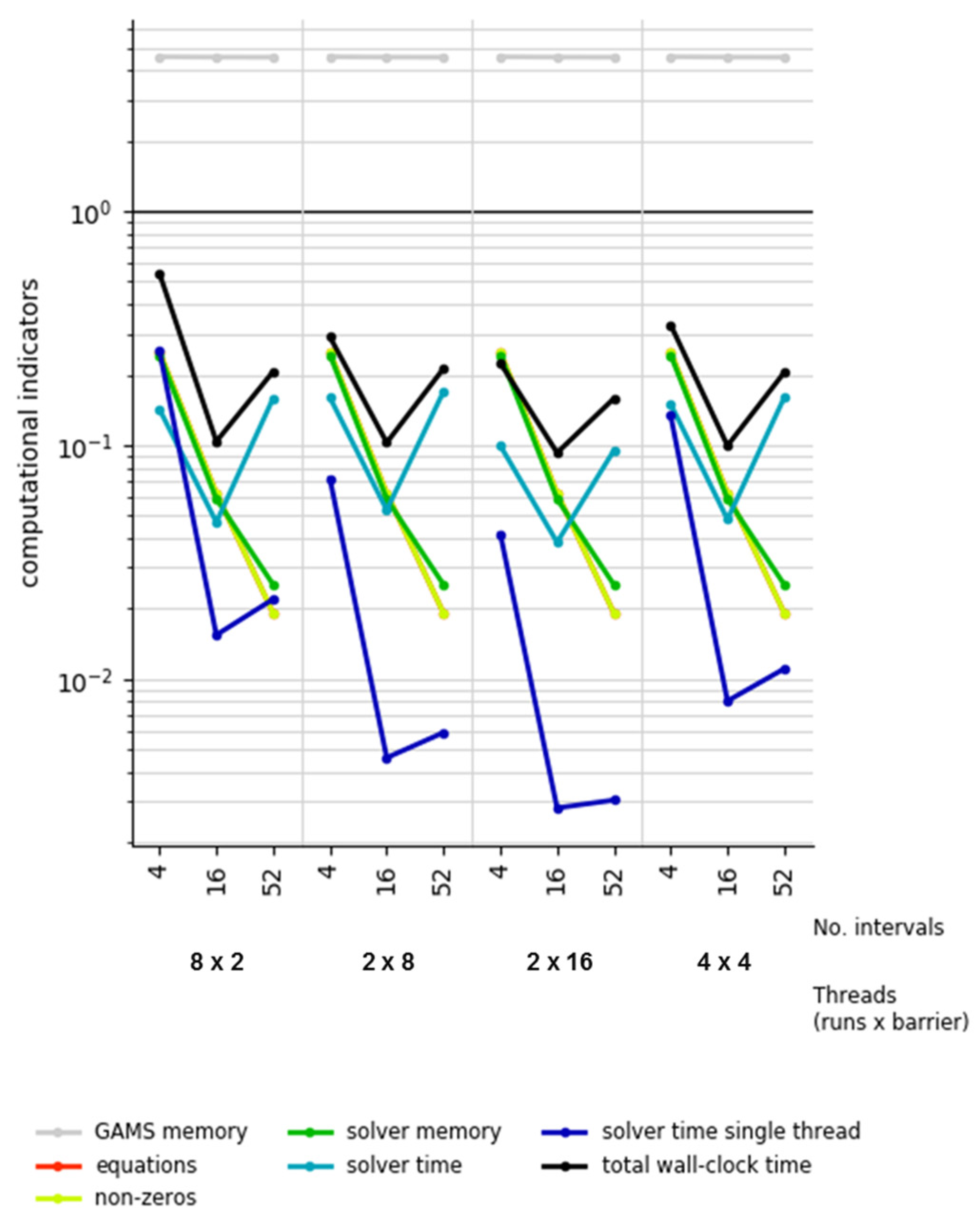
4.3.3. Temporal Zooming with Grid Computing
4.4. Temporal Aggregation Using Feed-in Time Series Based on Multiple Weather Years
5. Discussion
5.1. Summary
5.2. Into Context
5.3. Limitations
5.4. Methodological Improvements
- (1)
- Improved performance can be gained by running the independent model parts (such as the time intervals in case of grid computing presented in 0) on different computers. By this means, the drawback of being limited to memory and CPU resources of shared memory machines could be overcome. In this context, for a better coordination and utilization of available computing resources the application of workload managers such as Slurm [97] would be beneficial.
- (2)
- Improved accuracy can be reached by an extension to an exact decomposition approach that decomposes the temporal scale. However, this requires additional source code adaptions. For instance, in case of Benders decomposition, the distribution of emission budgets to the respective intervals needs to be realized by interval specific variables necessary to create benders cuts. Additionally, it can be expected that due to the need of an iterative execution of master and sub-problems the total computing time would significantly increase. Taking into account the best achievable speed-up of 10 of temporal zooming compared to simply solving the monolithic model, there is only a little room for improvements which may be disproportionate to the implantation effort required.
5.5. Practical Implications
6. Conclusions
- the “objective value” of the optimization problem,
- “power supply” of different electricity generation and load balancing technologies as well as, if appropriate,
- “added capacities” of storage and electricity transmission
Author Contributions
Funding
Acknowledgments
Conflicts of Interest
References
- Baños, R.; Manzano-Agugliaro, F.; Montoya, F.G.; Gil, C.; Alcayde, A.; Gómez, J. Optimization methods applied to renewable and sustainable energy: A review. Renew. Sustain. Energy Rev. 2011, 15, 1753–1766. [Google Scholar] [CrossRef]
- Paltsev, S. Energy scenarios: The value and limits of scenario analysis. Wiley Interdiscip. Rev. Energy Environ. 2017, 6. [Google Scholar] [CrossRef]
- Ventosa, M.; Baíllo, Á.; Ramos, A.; Rivier, M. Electricity market modeling trends. Energy Policy 2005, 33, 897–913. [Google Scholar] [CrossRef]
- Kagiannas, A.G.; Askounis, D.T.; Psarras, J. Power generation planning: A survey from monopoly to competition. Int. J. Electr. Power Energy Syst. 2004, 26, 413–421. [Google Scholar] [CrossRef]
- Wu, F.; Zheng, F.L.; Wen, F.S. Transmission investment and expansion planning in a restructured electricity market. Energy 2006, 31, 954–966. [Google Scholar] [CrossRef]
- Zhu, J.; Hu, K.; Lu, X.; Huang, X.; Liu, K.; Wu, X. A review of geothermal energy resources, development, and applications in China: Current status and prospects. Energy 2015, 93, 466–483. [Google Scholar] [CrossRef]
- Oree, V.; Hassen, S.Z.S.; Fleming, P.J. Generation expansion planning optimisation with renewable energy integration: A review. Renew. Sustain. Energy Rev. 2017, 69, 790–803. [Google Scholar] [CrossRef]
- Frank, S.; Steponavice, I.; Rebennack, S. Optimal power flow: A bibliographic survey I. Energy Syst. 2012, 3, 221–258. [Google Scholar] [CrossRef]
- Quintero, J.; Zhang, H.; Chakhchoukh, Y.; Vittal, V.; Heydt, G.T. Next Generation Transmission Expansion Planning Framework: Models, Tools, and Educational Opportunities. IEEE Trans. Power Syst. 2014, 29, 1911–1918. [Google Scholar] [CrossRef]
- Haas, J.; Cebulla, F.; Cao, K.; Nowak, W.; Palma-Behnke, R.; Rahmann, C.; Mancarella, P. Challenges and trends of energy storage expansion planning for flexibility provision in low-carbon power systems—A review. Renew. Sustain. Energy Rev. 2017, 80, 603–619. [Google Scholar] [CrossRef]
- Eurostat European Commission Eurostat. NUTS-Nomenclature of Territorial Units for Statistics; Eurostat European Commission Eurostat: Brussels, Belgium, 2017. [Google Scholar]
- Kondziella, H.; Bruckner, T. Flexibility requirements of renewable energy based electricity systems—A review of research results and methodologies. Renew. Sustain. Energy Rev. 2016, 53, 10–22. [Google Scholar] [CrossRef]
- Brouwer, A.S.; Broek, M.; van den Zappa, W.; Turkenburg, W.C.; Faaij, A. Least-cost options for integrating intermittent renewables in low-carbon power systems. Appl. Energy 2016, 161, 48–74. [Google Scholar] [CrossRef]
- Weigt, H.; Jeske, T.; Leuthold, F.; von Hirschhausen, C. Take the long way down: Integration of large-scale North Sea wind using HVDC transmission. Energy Policy 2010, 38, 3164–3173. [Google Scholar] [CrossRef]
- Bussar, C.; Stöcker, P.; Cai, Z.; Moraes, M., Jr.; Magnor, D.; Wiernes, P.; Bracht, N.; van Moser, A.; Sauer, D.U. Large-scale integration of renewable energies and impact on storage demand in a European renewable power system of 2050 Sensitivity study. J. Energy Storage 2016, 6, 1–10. [Google Scholar] [CrossRef]
- Loulou, R.; Labriet, M. ETSAP-TIAM: The TIMES integrated assessment model Part I: Model structure. Comput. Manag. Sci. 2007, 5, 7–40. [Google Scholar] [CrossRef]
- Deckmann, S.; Pizzolante, A.; Monticelli, A.; Stott, B.; Alsac, O. Studies on Power System Load Flow Equivalencing. IEEE Trans. Power Appar. Syst. 1980, 99, 2301–2310. [Google Scholar] [CrossRef]
- Dorfler, F.; Bullo, F. Kron Reduction of Graphs with Applications to Electrical Networks. IEEE Trans. Circuits Syst. I Regul. Pap. 2013, 60, 150–163. [Google Scholar] [CrossRef]
- Shayesteh, E.; Hamon, C.; Amelin, M.; Söder, L. REI method for multi-area modeling of power systems. Int. J. Electr. Power Energy Syst. 2014, 60, 283–292. [Google Scholar] [CrossRef]
- Shi, D.; Tylavsky, D.J. A Novel Bus-Aggregation-Based Structure-Preserving Power System Equivalent. Power Syst. IEEE Trans. Power Syst. 2015, 30, 1977–1986. [Google Scholar] [CrossRef]
- Oh, H. Optimal Planning to Include Storage Devices in Power Systems. Power Syst. IEEE Trans. 2011, 26, 1118–1128. [Google Scholar] [CrossRef]
- Corcoran, B.A.; Jenkins, N.; Jacobson, M.Z. Effects of aggregating electric load in the United States. Energy Policy 2012, 46, 399–416. [Google Scholar] [CrossRef]
- Schaber, K.; Steinke, F.; Hamacher, T. Transmission grid extensions for the integration of variable renewable energies in Europe: Who benefits where? Energy Policy 2012, 43, 123–135. [Google Scholar] [CrossRef]
- Anderski, T.; Surmann, Y.; Stemmer, S.; Grisey, N.; Momo, E.; Leger, A.-C.; Betraoui, B.; Roy, P.V. Modular Development Plan of the Pan-European Transmission System 2050-European Cluster Model of the Pan-European Transmission Grid; European Union: Brussels, Belgium, 2014. [Google Scholar]
- Hörsch, J.; Brown, T. The role of spatial scale in joint optimisations of generation and transmission for European highly renewable scenarios. In Proceedings of the 2017 14th International Conference on the European Energy Market (EEM), Dresden, Germany, 6–9 June 2017; pp. 1–7. [Google Scholar]
- Pfenninger, S. Dealing with multiple decades of hourly wind and PV time series in energy models: A comparison of methods to reduce time resolution and the planning implications of inter-annual variability. Appl. Energy 2017, 197, 1–13. [Google Scholar] [CrossRef]
- Zerrahn, A.; Schill, W.-P. Long-run power storage requirements for high shares of renewables: Review and a new model. Renew. Sustain. Energy Rev. 2017, 79, 1518–1534. [Google Scholar] [CrossRef]
- Deane, J.P.; Drayton, G.; Gallachóir, B.P.Ó. The impact of sub-hourly modelling in power systems with significant levels of renewable generation. Appl. Energy 2014, 113, 152–158. [Google Scholar] [CrossRef]
- O’Dwyer, C.; Flynn, D. Using energy storage to manage high net load variability at sub-hourly time-scales. IEEE Trans. Power Syst. 2015, 30, 2139–2148. [Google Scholar] [CrossRef]
- Pandzzic, H.; Dvorkin, Y.; Wang, Y.; Qiu, T.; Kirschen, D.S. Effect of time resolution on unit commitment decisions in systems with high wind penetration. In Proceedings of the PES General Meeting Conference Exposition, National Harbor, MD, USA, 27–31 July 2014; pp. 1–5. [Google Scholar]
- Ludig, S.; Haller, M.; Schmid, E.; Bauer, N. Fluctuating renewables in a long-term climate change mitigation strategy. Energy 2011, 36, 6674–6685. [Google Scholar] [CrossRef]
- Leuthold, F.U.; Weigt, H.; von Hirschhausen, C. A Large-Scale Spatial Optimization Model of the European Electricity Market. Netw. Spat. Econ. 2012, 12, 75–107. [Google Scholar] [CrossRef]
- Wogrin, S.; Duenas, P.; Delgadillo, A.; Reneses, J. A New Approach to Model Load Levels in Electric Power Systems With High Renewable Penetration. IEEE Trans. Power Syst. 2014, 29, 2210–2218. [Google Scholar] [CrossRef]
- Green, R.; Staffell, I.; Vasilakos, N. Divide and Conquerk-Means Clustering of Demand Data Allows Rapid and Accurate Simulations of the British Electricity System. IEEE Trans. Eng. Manag. 2014, 61, 251–260. [Google Scholar] [CrossRef]
- Nahmmacher, P.; Schmid, E.; Hirth, L.; Knopf, B. Carpe diem: A novel approach to select representative days for long-term power system modeling. Energy 2016, 112, 430–442. [Google Scholar] [CrossRef]
- Spiecker, S.; Vogel, P.; Weber, C. Evaluating interconnector investments in the north European electricity system considering fluctuating wind power penetration. Energy Econ. 2013, 37, 114–127. [Google Scholar] [CrossRef]
- Haydt, G.; Leal, V.; Pina, A.; Silva, C.A. The relevance of the energy resource dynamics in the mid/long-term energy planning models. Renew. Energy 2011, 36, 3068–3074. [Google Scholar] [CrossRef]
- Kotzur, L.; Markewitz, P.; Robinius, M.; Stolten, D. Impact of different time series aggregation methods on optimal energy system design. Renew. Energy 2018, 117, 474–487. [Google Scholar] [CrossRef]
- Merrick, J.H. On representation of temporal variability in electricity capacity planning models. Energy Econ. 2016, 59, 261–274. [Google Scholar] [CrossRef]
- Mitra, S.; Sun, L.; Grossmann, I.E. Optimal scheduling of industrial combined heat and power plants under time-sensitive electricity prices. Energy 2013, 54, 194–211. [Google Scholar] [CrossRef]
- Frew, B.A.; Becker, S.; Dvorak, M.J.; Andresen, G.B.; Jacobson, M.Z. Flexibility mechanisms and pathways to a highly renewable US electricity future. Energy 2016, 101, 65–78. [Google Scholar] [CrossRef]
- Palmintier, B.S. Incorporating Operational Flexibility into Electric Generation Planning: Impacts and Methods for System Design and Policy Analysis; Massachusetts Institute of Technology: Cambridge, MA, USA, 2013. [Google Scholar]
- Poncelet, K.; Delarue, E.; Six, D.; Duerinck, J.; D’haeseleer, W. Impact of the level of temporal and operational detail in energy-system planning models. Appl. Energy 2016, 162, 631–643. [Google Scholar] [CrossRef]
- Raichur, V.; Callaway, D.S.; Skerlos, S.J. Estimating Emissions from Electricity Generation Using Electricity Dispatch Models: The Importance of System Operating Constraints. J. Ind. Ecol. 2016, 20, 42–53. [Google Scholar] [CrossRef]
- Stoll, B.; Brinkman, G.; Townsend, A.; Bloom, A. Analysis of Modeling Assumptions Used in Production Cost Models for Renewable Integration Studies; National Renewable Energy Laboratory (NREL): Golden, CO, USA, 2016.
- Cebulla, F.; Fichter, T. Merit order or unit-commitment: How does thermal power plant modeling affect storage demand in energy system models? Renew. Energy 2017, 105, 117–132. [Google Scholar] [CrossRef]
- Abrell, J.; Kunz, F.; Weigt, H. Start Me Up: Modeling of Power Plant Start-Up Conditions and Their Impact on Prices; Working Paper; Universität Dresden: Dresden, Germany, 2008. [Google Scholar]
- Langrene, N.; Ackooij, W.; van Breant, F. Dynamic Constraints for Aggregated Units: Formulation and Application. Power Syst. IEEE Trans. 2011, 26, 1349–1356. [Google Scholar] [CrossRef]
- Munoz, F.D.; Sauma, E.E.; Hobbs, B.F. Approximations in power transmission planning: Implications for the cost and performance of renewable portfolio standards. J. Regul. Econ. 2013, 43, 305–338. [Google Scholar] [CrossRef]
- Nolden, C.; Schönfelder, M.; Eßer-Frey, A.; Bertsch, V.; Fichtner, W. Network constraints in techno-economic energy system models: Towards more accurate modeling of power flows in long-term energy system models. Energy Syst. 2013, 4, 267–287. [Google Scholar] [CrossRef][Green Version]
- Romero, R.; Monticelli, A. A hierarchical decomposition approach for transmission network expansion planning. IEEE Trans. Power Syst. 1994, 9, 373–380. [Google Scholar] [CrossRef]
- Gils, H.C. Balancing of Intermittent Renewable Power Generation by Demand Response and Thermal Energy Storage; Universität Stuttgart: Stuttgart, Germany, 2015. [Google Scholar]
- Haikarainen, C.; Pettersson, F.; Saxen, H. A decomposition procedure for solving two-dimensional distributed energy system design problems. Appl. Therm. Eng. 2016. [Google Scholar] [CrossRef]
- Scholz, A.; Sandau, F.; Pape, C. A European Investment and Dispatch Model for Determining Cost Minimal Power Systems with High Shares of Renewable Energy. Oper. Res. Proc. 2016. [Google Scholar] [CrossRef]
- Babrowski, S.; Heffels, T.; Jochem, P.; Fichtner, W. Reducing computing time of energy system models by a myopic approach. Energy Syst. 2013. [Google Scholar] [CrossRef]
- Tuohy, A.; Denny, E.; O’Malley, M. Rolling Unit Commitment for Systems with Significant Installed Wind Capacity. IEEE Lausanne Power Tech. 2007. [Google Scholar] [CrossRef]
- Barth, R.; Brand, H.; Meibom, P.; Weber, C. A Stochastic Unit-commitment Model for the Evaluation of the Impacts of Integration of Large Amounts of Intermittent Wind Power. In Proceedings of the 2006 International Conference on Probabilistic Methods Applied to Power Systems, Stockholm, Sweden, 11–15 June 2006; pp. 1–8. [Google Scholar]
- Silvente, J.; Kopanos, G.M.; Pistikopoulos, E.N.; Espuña, A. A rolling horizon optimization framework for the simultaneous energy supply and demand planning in microgrids. Appl. Energy 2015, 155, 485–501. [Google Scholar] [CrossRef]
- Marquant, J.F.; Evins, R.; Carmeliet, J. Reducing Computation Time with a Rolling Horizon Approach Applied to a {MILP} Formulation of Multiple Urban Energy Hub System. Procedia Comput. Sci. 2015, 51, 2137–2146. [Google Scholar] [CrossRef]
- Conejo, A.J.; Castillo, E.; Mínguez, R.; García-Bertrand, R. Decomposition Techniques in Mathematical Programming; Springer: Berlin, Germany, 2006. [Google Scholar]
- Flores-Quiroz, A.; Palma-Behnke, R.; Zakeri, G.; Moreno, R. A column generation approach for solving generation expansion planning problems with high renewable energy penetration. Electr. Power Syst. Res. 2016, 136, 232–241. [Google Scholar] [CrossRef]
- Virmani, S.; Adrian, E.C.; Imhof, K.; Mukherjee, S. Implementation of a Lagrangian relaxation based unit commitment problem. IEEE Trans. Power Syst. 1989, 4, 1373–1380. [Google Scholar] [CrossRef]
- Wang, Q.; McCalley, J.D.; Zheng, T.; Litvinov, E. Solving corrective risk-based security-constrained optimal power flow with Lagrangian relaxation and Benders decomposition. Int. J. Electr. Power Energy Syst. 2016, 75, 255–264. [Google Scholar] [CrossRef]
- Alguacil, N.; Conejo, A.J. Multiperiod optimal power flow using Benders decomposition. IEEE Trans. Power Syst. 2000, 15, 196–201. [Google Scholar] [CrossRef]
- Amjady, N.; Ansari, M.R. Hydrothermal unit commitment with {AC} constraints by a new solution method based on benders decomposition. Energy Convers. Manag. 2013, 65, 57–65. [Google Scholar] [CrossRef]
- Binato, S.; Pereira, M.V.F.; Granville, S. A new Benders decomposition approach to solve power transmission network design problems. IEEE Trans. Power Syst. 2001, 16, 235–240. [Google Scholar] [CrossRef]
- Esmaili, M.; Ebadi, F.; Shayanfar, H.A.; Jadid, S. Congestion management in hybrid power markets using modified Benders decomposition. Appl. Energy 2013, 102, 1004–1012. [Google Scholar] [CrossRef]
- Habibollahzadeh, H.; Bubenko, J.A. Application of Decomposition Techniques to Short-Term Operation Planning of Hydrothermal Power System. IEEE Trans. Power Syst. 1986, 1, 41–47. [Google Scholar] [CrossRef]
- Khodaei, A.; Shahidehpour, M.; Kamalinia, S. Transmission Switching in Expansion Planning. IEEE Trans. Power Syst. 2010, 25, 1722–1733. [Google Scholar] [CrossRef]
- Martínez-Crespo, J.; Usaola, J.; Fernández, J.L. Optimal security-constrained power scheduling by Benders decomposition. Electr. Power Syst. Res. 2007, 77, 739–753. [Google Scholar] [CrossRef][Green Version]
- Roh, J.H.; Shahidehpour, M.; Fu, Y. Market-Based Coordination of Transmission and Generation Capacity Planning. IEEE Trans. Power Syst. 2007, 22, 1406–1419. [Google Scholar] [CrossRef]
- Wang, S.J.; Shahidehpour, S.M.; Kirschen, D.S.; Mokhtari, S.; Irisarri, G.D. Short-term generation scheduling with transmission and environmental constraints using an augmented Lagrangian relaxation. IEEE Trans. Power Syst. 1995, 10, 1294–1301. [Google Scholar] [CrossRef]
- Wang, J.; Shahidehpour, M.; Li, Z. Security-Constrained Unit Commitment With Volatile Wind Power Generation. IEEE Trans. Power Syst. 2008, 23, 1319–1327. [Google Scholar] [CrossRef]
- Xin-gang, Z.; Tian-tian, F.; Lu, C.; Xia, F. The barriers and institutional arrangements of the implementation of renewable portfolio standard: A perspective of China. Renew. Sustain. Energy Rev. 2014, 30, 371–380. [Google Scholar] [CrossRef]
- Papavasiliou, A.; Oren, S.S.; Rountree, B. Applying high performance computing to transmission-constrained stochastic unit commitment for renewable energy integration. IEEE Trans. Power Syst. 2015, 30, 1109–1120. [Google Scholar] [CrossRef]
- McCarl, B.A. Speeding up GAMS Execution Time; Materials drawn from Advanced GAMS Class by Bruce A McCarl: College Station, TX, USA, 2000. [Google Scholar]
- Cao, K.-K.; Metzdorf, J.; Birbalta, S. Incorporating Power Transmission Bottlenecks into Aggregated Energy System Models. Sustainability 2018, 10, 1916. [Google Scholar] [CrossRef]
- Teruel, A.G. Perspestective of the Energy Transition: Technology Development and Investments under Uncertainty; Technical University of Munich: Munich, Germany, 2015. [Google Scholar]
- Egerer, J.; Gerbaulet, C.; Ihlenburg, R.; Kunz, F.; Reinhard, B.; von Hirschhausen, C.; Weber, A.; Weibezahn, J. Electricity Sector Data for Policy-Relevant Modeling: Data Documentation and Applications to the German and European Electricity Markets; Data Documentation; DIW: Berlin, Germany, 2014. [Google Scholar]
- Open Power System Data Data Package Time Series. Available online: https://data.open-power-system-data.org/time_series/2017-07-09 (accessed on 2 August 2017).
- Rippel, K.M.; Preuß, A.; Meinecke, M.; König, R. Netzentwicklungsplan 2030 Zahlen Daten Fakten; German Transmission System Operators: Berlin, Germany, 2017. [Google Scholar]
- Wiegmans, B. GridKit Extract of ENTSO-E Interactive Map; 2016. Available online: https://zenodo.org/record/55853 (accessed on 10 July 2017).
- Hofmann, F.; Hörsch, J.; Gotzens, F. FRESNA/Powerplantmatching: Python3 Adjustments; 2018. Available online: https://github.com/FRESNA/powerplantmatching (accessed on 3 July 2017).
- ENTSO-E Transparency Platform Cross-Border Commercial Schedule and Cross-Border Physical Flow. Available online: https://transparency.entsoe.eu/content/static_content/Static%20content/legacy%20data/legacy%20data2012.html 2012 (accessed on 29 June 2017).
- Gils, H.C.; Scholz, Y.; Pregger, T.; de Tena, D.L.; Heide, D. Integrated modelling of variable renewable energy-based power supply in Europe. Energy 2017, 123, 173–188. [Google Scholar] [CrossRef]
- Gils, H.C.; Simon, S. Carbon neutral archipelago-100% renewable energy supply for the Canary Islands. Appl. Energy 2017, 188, 342–355. [Google Scholar] [CrossRef]
- Gils, H.C.; Simon, S.; Soria, R. 100% Renewable Energy Supply for Brazil—The Role of Sector Coupling and Regional Development. Energies 2017, 10, 1859. [Google Scholar] [CrossRef]
- Cao, K.-K.; Gleixner, A.; Miltenberger, M. Methoden zur Reduktion der Rechenzeit linearer Optimierungsmodelle in der Energiewirtschaft? Eine Performance-Analyse. In Proceedings of the 14. Symposium Energieinnovation, Graz, Austria, 10–12 February 2016. [Google Scholar]
- Scholz, Y.; Gils, H.C.; Pietzcker, R.C. Application of a high-detail energy system model to derive power sector characteristics at high wind and solar shares. Energy Econ. 2017, 64, 568–582. [Google Scholar] [CrossRef]
- Gils, H.C.; Bothor, S.; Genoese, M.; Cao, K.-K. Future security of power supply in Germany–the role of stochastic power plant outages and intermittent generation. Int. J. Energy Res. 2018, 42, 1894–1913. [Google Scholar] [CrossRef]
- Pedregosa, F.; Varoquaux, G.; Gramfort, A.; Michel, V.; Thirion, B.; Grisel, O.; Blondel, M.; Prettenhofer, P.; Weiss, R.; Dubourg, V.; et al. Scikit-learn: Machine Learning in Python. J. Mach. Learn. Res. 2011, 12, 2825–2830. [Google Scholar]
- IBM. IBM Deterministic Time, Release Notes for IBM CPLEX Optimizer for z/OS V12.5; IBM: Armonk, NY, USA, 2013. [Google Scholar]
- IBM. IBM ILOG CPLEX Optimization StudioCPLEX User’s Manual; IBM Corporation: Armonk, NY, USA, 2017. [Google Scholar]
- Ramos, A. Good Optimization Modeling Practices with GAMS; Lecture; Universidad Pontificia Comillas: Madrid, Spain, 2018. [Google Scholar]
- McCarl, B. Bruce McCarl’s GAMS Newsletter Number 41. Available online: https://www.gams.com/fileadmin/community/mccarlarchive/news41.pdf (accessed on 10 June 2019).
- Breuer, T. Contribution of HPC to the BEAM-ME project. In Implementation of Acceleration Strategies from Mathematics and Computational Sciences for Optimizing Energy System Models; Final Workshop; The BEAM-ME Project: Aachen, Germany, 2019. [Google Scholar]
- Slurm Workload Manager. Available online: https://slurm.schedmd.com (accessed on 6 July 2019).
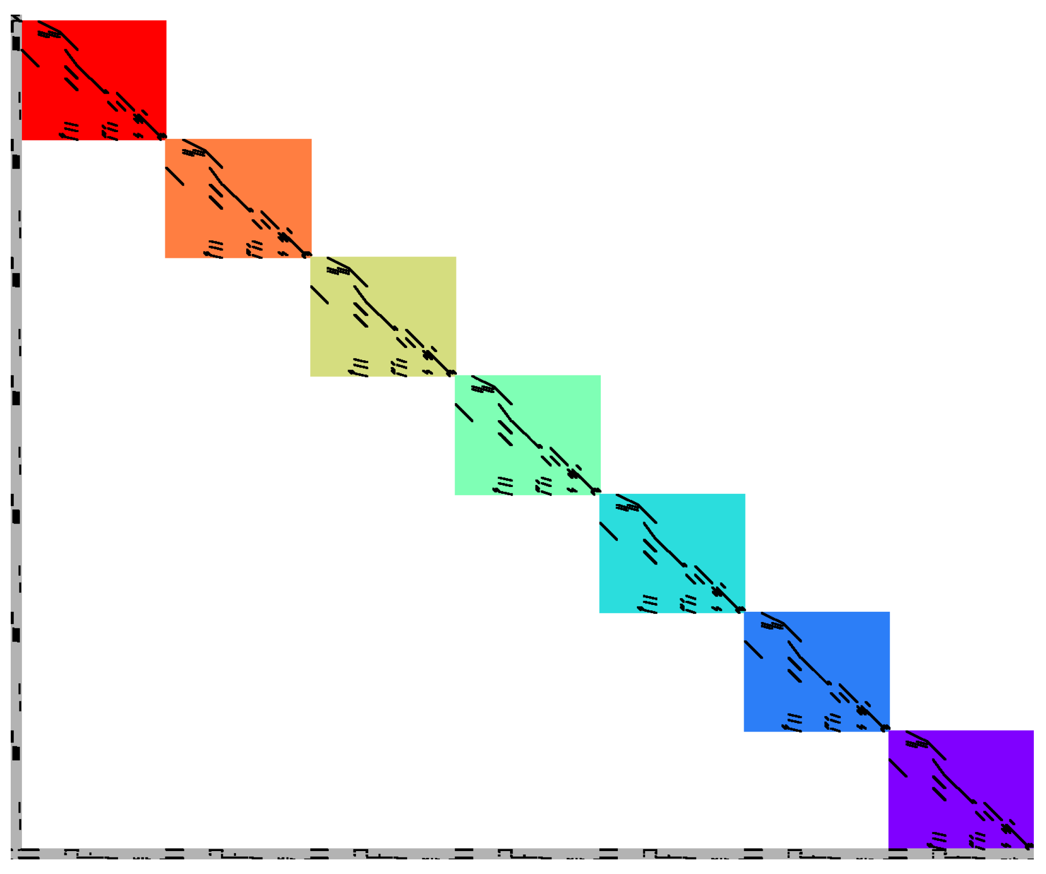
- Breuer, T.; Bussieck, M.; Cao, K.-K.; Cebulla, F.; Fiand, F.; Gils, H.C.; Gleixner, A.; Khabi, D.; Koch, T.; Rehfeldt, D.; et al. Optimizing Large-Scale Linear Energy System Problems with Block Diagonal Structure by Using Parallel Interior-Point Methods. In Operations Research Proceedings 2017; Kliewer, N., Ehmke, J.F., Borndörfer, R., Eds.; Springer: Berlin, Germany, 2018. [Google Scholar]


| Dimension | Model Characteristic | Descriptive Characteristic | Example | |
|---|---|---|---|---|
| Time | Set of time steps | Short-term (sub-annual operation) | Long-term (configuration/investment) | |
| Temporal resolution | hourly | each 5 years | ||
| Planning horizon | one year | from 2020 until 2050 | ||
| Space | Set of regions | Spatial resolution | Administrative regions (e.g., NUTS3 [11]) | |
| Geographical scope | European Union | |||
| Technology | Variables and constraints per technology | Technological detail | Consideration of start-up behavior, minimum downtimes | |
| Set of technologies | Technological diversity | Power and heat generation, transmission grids and storage facilities | ||
| Authors | Math. Problem Type | Descriptive Problem Type | Decomposed Model Scale | Decomposition Technique | Decomposition Purpose |
|---|---|---|---|---|---|
| Alguacil and Conejo [64] | MIP/NLP | Plant and grid operation | Time, single sub-problem | Benders decomposition | Decoupling of UC and multi-period DC-OPF * |
| Amjady and Ansari [65] | MIP/NLP | Plant operation | Benders decomposition | Decoupling of UC and AC-OPF ** | |
| Binato et al. [66] | MIP/LP | TEP | Benders decomposition | Decoupling of discrete investment decisions and DC-OPF | |
| Esmaili et al. [67] | NLP/LP | Grid operation | Benders decomposition | Decoupling of AC-OPF and congestion constraints | |
| Flores-Quiroz et al. [61] | MIP/LP | GEP | Time, 1-31 sub-problems, sequentially solved | Dantzig-Wolfe decomposition | Decoupling of discrete investment and UC |
| Habibollahzadeh et al. [68] | MIP/LP | Plant operation | Benders decomposition | Decoupling of UC and ED | |
| Khodaei et al. [69] | MIP/LP | GEP-TEP | Time, two sub-problem types, sequentially solved | Benders decomposition | Decoupling of discrete investments into generation and transmission capacity, security constraints and DC-OPF |
| Martinez-Crespo et al. [70] | MIP/NLP | Plant and grid operation | Time, 24 sub-problems, sequentially solved | Benders decomposition | Decoupling of UC and security constraint AC-OPF |
| Roh and Shahidehpour [71] | MIP/LP | GEP-TEP | Time, up to 10 × 4 sub-problems, sequentially solved | Benders decomposition and Lagrangian Relaxation | Decoupling of discrete investments into generation and transmission capacity, security constraints and DC-OPF |
| Virmani et al. [62] | LP/MIP | Plant operation | Technology (generation units), up to 20 sub-problems, sequentially solved | Lagrangian Relaxation | Decoupling of unit specific(UC) and cross-park (ED) constraints |
| Wang et al. [72] | LP/MIP | Plant and grid operation | Space, 26 sub-problems, sequentially solved | Lagrangian Relaxation | Decoupling of DC-OPF and UC |
| Wang et al. [73] | MIP/NLP | Plant and grid operation | Scenarios and time, 10 × 4 sub-problems, sequentially solved | Benders decomposition | Decoupling of UC, scenario specific system adequacy constraints and network security constraints |
| Wang et al. [63] | LP | Plant and grid operation | Technology (circuits) and time (contingencies), two sub-problem types, sequentially solved | Lagrangian Relaxation and Benders decomposition | Decoupling of DC-OPF, system risk constraints and network security constraints |
| Model Name | REMix | |||
|---|---|---|---|---|
| Author (Institution) | German Aerospace Center (DLR), Institute of Engineering Thermodynamics | |||
| Model type | Linear programing Minimization of total costs for system operation and expansion Economic dispatch/optimal dc power flow with expansion of storage and transmission capacities | |||
| Sectoral focus | Electricity | |||
| Geographical focus | Germany | |||
| Spatial resolution | 488 nodes | |||
| Analyzed year (scenario) | 2030 | |||
| Temporal resolution | 8760 time steps (hourly) | |||
| Input-parameters: | Dependencies | |||
| Temporal | Technical | Spatial | ||
| Conversion efficiencies [78] | x | |||
| Operational costs [78] | x | |||
| Fuel prices and emission allowances [79] | x | |||
| Electricity load profiles [80] | x | x | ||
| Capacities of power generation, storage and grid transfer capacities and annual electricity demand [81,82,83] | x | x | ||
| Renewable energy resources feed-in profiles | x | x | x | |
| Import and export time series for cross-border power flows [84] | x | x | ||
| Evaluated output parameters | System costs (objective value) | |||
| Generated power | x | x | ||
| Added storage/transmission capacities | x | |||
| Storage levels | x | x | x | |
| Processor | Available Threads | Available Memory |
|---|---|---|
| Dual Intel Xeon Platinum 8168 | 2x 24 @ 2.7 GHz | 192 GB |
| Intel Xeon Gold 6148 | 2x 40 @ 2.4 GHz | 368 GB |
| Original Model Instance Name | Applied Speed-Up Approaches | Number of Variables | Number of Constraints | Number of Non-Zeros |
|---|---|---|---|---|
| REMix Dispatch |
| 30,579,396 | 9,214,488 | 69,752,951 |
| REMix Expansion |
| 43,169,135 | 32,805,201 | 137,967,269 |
| Speed-Up Approach | Parameter | |
|---|---|---|
| Name | Evaluated Range | |
| Spatial aggregation | number of regions (clusters) | {1, 5, 18, 50, 100, 150, 200, 250, 300, 350, 400, 450, 488} |
| Down-sampling | temporal resolution | {1, 2, 3, 4, 6, 8, 12, 24, 48, 168, 1095, 4380} |
| Rolling horizon dispatch | number of intervals | {4, 16, 52,365} |
| overlap size | {1%, 2%, 4%, 10%} | |
| Temporal zooming (sequential) | number of intervals | {4, 16, 52} |
| temporal resolution of down-sampled run | {4, 8, 24} | |
| Temporal zooming (grid computing) | number of intervals | {4, 16, 52} |
| number barrier threads | {2, 4, 8, 16} | |
| number of parallel runs | {2, 4, 8, 16} | |
| temporal resolution of down-sampled run | {8, 24} | |
| Speed-Up Approach | Sufficient Speed-Up (Model Instance) | Accuracy | |
| Average | Worst (Affected Indicator) | ||
| Spatial aggregation | |||
| “REMix Dispatch” | >4 (100 regions) | >95% | >70% (power transmission) |
| “REMix Expansion” | >8 (150 regions) | >95% | >70% (transmission expansion) |
| Down-sampling | |||
| “REMix Dispatch” | >6 (2190 time steps) | >97% | >81% (storage utilization) |
| “REMix Expansion” | >10 (2190 time steps) | >97% | >87% (storage utilization) |
| Rolling horizon dispatch | ≈2.5 (16 intervals) | >96% | >87% (storage utilization) |
| Temporal zooming (sequential) | >8 (1095 time steps/16 intervals) | >93% | >69% (storage expansion) |
| Temporal zooming (grid computing) | >10 (1095 time steps/16 intervals) | >92% | >68% (storage expansion) |
© 2019 by the authors. Licensee MDPI, Basel, Switzerland. This article is an open access article distributed under the terms and conditions of the Creative Commons Attribution (CC BY) license (http://creativecommons.org/licenses/by/4.0/).
Share and Cite
Cao, K.-K.; von Krbek, K.; Wetzel, M.; Cebulla, F.; Schreck, S. Classification and Evaluation of Concepts for Improving the Performance of Applied Energy System Optimization Models. Energies 2019, 12, 4656. https://doi.org/10.3390/en12244656
Cao K-K, von Krbek K, Wetzel M, Cebulla F, Schreck S. Classification and Evaluation of Concepts for Improving the Performance of Applied Energy System Optimization Models. Energies. 2019; 12(24):4656. https://doi.org/10.3390/en12244656
Chicago/Turabian StyleCao, Karl-Kiên, Kai von Krbek, Manuel Wetzel, Felix Cebulla, and Sebastian Schreck. 2019. "Classification and Evaluation of Concepts for Improving the Performance of Applied Energy System Optimization Models" Energies 12, no. 24: 4656. https://doi.org/10.3390/en12244656
APA StyleCao, K.-K., von Krbek, K., Wetzel, M., Cebulla, F., & Schreck, S. (2019). Classification and Evaluation of Concepts for Improving the Performance of Applied Energy System Optimization Models. Energies, 12(24), 4656. https://doi.org/10.3390/en12244656