Optimal Decomposition and Reconstruction of Discrete Wavelet Transformation for Short-Term Load Forecasting

Abstract

To achieve high accuracy in prediction, a load forecasting algorithm must model various consumer behaviors in response to weather conditions or special events. Different triggers will have various effects on different customers and lead to difficulties in constructing an adequate prediction model due to non-stationary and uncertain characteristics in load variations. This paper proposes an open-ended model of short-term load forecasting (STLF) which has general prediction ability to capture the non-linear relationship between the load demand and the exogenous inputs. The prediction method uses the whale optimization algorithm, discrete wavelet transform, and multiple linear regression model (WOA-DWT-MLR model) to predict both system load and aggregated load of power consumers. WOA is used to optimize the best combination of detail and approximation signals from DWT to construct an optimal MLR model. The proposed model is validated with both the system-side data set and the end-user data set for Independent System Operator-New England (ISO-NE) and smart meter load data, respectively, based on Mean Absolute Percentage Error (MAPE) criterion. The results demonstrate that the proposed method achieves lower prediction error than existing methods and can have consistent prediction of non-stationary load conditions that exist in both test systems. The proposed method is, thus, beneficial to use in the energy management system.

1. Introduction

Necessity to construct a short-term load forecasting (STLF) model that has flexible applications at the system’s level and end user’s level grows rapidly by the common implementation of a future ahead bidding system, such as day-ahead demand response programs. System level refers to the electricity utilities, such as medium-voltage level customers, the distribution system, or aggregated residential users in one region. End-user’s level refers to the single residential load, apartment user, or a small-scale distribution user. End-user’s load characteristic has more variety than system’s level because it is strongly related to the user’s behavior, which is hard to model.

Both system and end-user data sets are necessary to have an accurate load prediction model to support further process, such as energy utilization [1], microgrid scheduling [2], and system demand analysis [3]. Habib et al. [1] applied the load prediction result to improve the energy and batteries utilization in hybrid power system, while Jin et al. [2] designed a load prediction which is fed to determine the optimal scheduling of distributed energy resources and microgrid of a smart building. Meanwhile, He et al. [3] used the load prediction accuracy derived from decoupling relation between electricity consumption and economic growth.

To have an accurate STLF method, several approaches estimate the load patterns and non-stationary part of load signal by modeling the user behavior and use signal decomposition to extract the non-stationary part of load signal. The user behavior model is built to estimate the exact load signals by considering various inputs, such as user daily schedules, as investigated by Stephen et al. [4] and Sajjad et al. [5], while Perfumo et al. [6] used specific temperature formulation. Another way to investigate user behavior is by using non-intrusive load monitoring to know status of each set of appliances as proposed by Welikala et al. [7]. However, information to build user behavior is scarcer in the wide area data set and driven by the seasonal effect of the time series, a fact that makes this approach less attractive, as applied in the work of Kong et al. [8], Xie et al. [9], and Erdinc et al. [10]. In contrast to modeling user behavior, the decomposition method is built after the load inputs are determined. Signal decomposition is used to smoothen the load variations, by using discrete wavelet transform (DWT), so that the input load pattern can be decomposed into low- and high-frequency parts of sub-signals for the input variables formulated.

To construct a closely fitting model of the load, a ubiquitous implementation of DWT is strongly related to proper selection of both the decomposition level and type of wavelet. Among the types of wavelet, Daubechies is well known due to its practicality in multiresolution signal application in which there is flexibility in analyzing the content of the signal. Li et al. [11], Chen et al. [12], and Reis and Alves da Silva [13] use the fourth order Daubechies (Db4) to predict the electric load with different decomposition levels of 3 to 5. Meanwhile, Guan et al. [14] and Li et al. [15] use the Daubechies types varying between Db1 to Db3 and the decomposition level of level-2. Bashir and El-Hawary [16] use Db2 with level-2 to reflect the uncertain factors on daily load characteristics. A particle swarm optimization (PSO) algorithm is then employed to adjust the weights of the artificial neural network (ANN) in the training process.

In addition to selection of the DWT’s decomposition level and type of wavelet, arrangement of the correct related exogenous inputs is necessary. Arrangement of input variables is mainly based on various weather information, lagged historical data, or an ensemble of sub-signals after wavelet decomposition. Pandey et al. [17] use conditional mutual information-based feature selection to extract information of the built wavelet models before assembling those models into a final prediction model. The prediction model designed by Chen et al. [12] is built based on Db4 and uses a similar day’s load as the input. A forecasting method proposed by Guan et al. [14] uses 12 dedicated models with two levels of decomposition and boundary of Daubechies type varying from Db1 to Db3. The problem of selecting input variables becomes more difficult when every related exogenous factor is added to the prediction model. Thus, this paper takes the idea of using correlation analysis and statistical t-test on the common related weather information to carefully select them.

ANNs can be used to predict load by several input variables, such as month, hour, day, the demand for same hour in the previous week, the demand of first- and second-forecasting hours, weighted temperature, humidity, and power demand pattern, as applied by Kong et al. [8]. Within a day of prediction horizon, some of the methods need to build separate ANN model for each hour as shown by Chen et al. [12] and Guan et al. [14] or using decomposed signal as proposed by Rocha Reis and Alves da Silva [13]. Guan et al. [14] proposed a prediction interval in which the decomposition needs to filter out the high-frequency part of the signal to smoothen the load variation. Li et al. [15] indicate the usage of the predetermined wavelet component and decomposition level cannot always improve the performance of prediction model. In addition, manual tuning of a hidden layer in an ANN cannot guarantee a general performance in a prediction model either, when it is used in another data set. Thus, to accommodate the problems with how to automatically select proper parameters for an accurate model, an optimal tuning algorithm is necessary.

To generalize the application of the load forecasting method, the prediction model must have accuracy in both system and end-user data sets. Sun et al. [18] use wavelet neural network (WNN) and load distribution factor to find suitable wavelet type varying from Db2 to Db20 for irregular and regular nodes of load flow in distribution system, respectively. The method uses two decomposition levels and trains each decomposed signal in separate networks. However, the method fails to keep its prediction accuracy for the smart meter load due to the unpredicted behavior of an end-user affecting the load variation.

From the related works, the prediction model of STLF strongly depends on two key variables, which are the predictors and structure of the prediction algorithm. The predictors are designed to capture the load characteristics, while the structure of prediction algorithm determines the close-fitting process between targeted output and the prediction result. Integrating the evolutionary algorithm becomes the prominent way to address the issue to find optimal structure of prediction algorithm. He et al. [3] show that an improved particle swarm optimization-extreme learning machine (IPSO-ELM) can optimize the weight in an ELM, which improves the overall load prediction result. Bashir and El-Hawary [16] used PSO to the ANN model combined with wavelet decomposition to successfully extract redundant information from the load and achieve high precision.

For the design of highly correlated predictors to closely-fit the actual load, it is proved by Stephen et al. [4] that the ensemble forecast from Autoregressive Integrated Moving Average (ARIMA), ANN, persistent forecast, and Gaussian load profile can improve the mean absolute percentage error (MAPE) from 18.56% to 11.13% for the residential load. In Kong et al. [8], long short-term memory is used in the residential load forecasting to improve the performance by 21.99% of MAPE. Pandey et al. [17] apply the WNN to Canadian utility load data, in which the predictors are grouped into seasons, to achieve 1.033% of MAPE on average. Thus, the proposed method adheres to the related works and investigates how to design the optimal predictors and prediction structure through several preconditioning schemes and discrete wavelet decomposition.

This paper proposes a one-day ahead hourly prediction model that integrates multiple linear regression (MLR) and discrete wavelet transform (DWT) optimized by using the whale optimization algorithm (WOA). The WOA is proposed by Mirjalili and Lewis [19] as a novel meta-heuristic optimization algorithm which mimics the social behavior of humpback whales to find a global optimum solution. Compared to the other optimization algorithms, WOA converges fast and tunes only a few parameters to approach an optimal solution. The proposed model provides a more accurate prediction method that closely fits system-side loads and aggregated loads at downstream level (end-user). Instead of using ANN, the proposed method is suitable for real time application because it uses MLR that requires less time while dealing with multiple inputs. Multiple weather attributes and load data conditions are employed as the input of MLR. Based on Daubechies type wavelet, DWT is used to decompose a non-stationary signal into several components. The signal is independently decomposed to the set of Daubechies levels and types by handling the selected decomposition coefficients, while the remaining coefficients are replaced with zero. Based on this scheme, the signal can be extracted with its unique characteristics reflected by individual approximation and detail components. Then, WOA is used to optimize the combination of signals for constructing a prediction model.

The proposed method is validated in both system-side and end-user data sets, respectively, associated with actual weather information. The state-of-the-art features of the proposed method include:

• Accurate and consistent implementation of STLF is achieved in both system-side and aggregated end-user data sets by integrating WOA-based DWT in the MLR model.
• Due to the superior optimization ability of WOA, the best of DWT is implemented for more accurate prediction with more sensible load pattern reconstruction and more flexibility to interpret unique load characteristics of each data set.
• The simple design is targeted yet does not lose accuracy of prediction via best reconstructing signals of DWT and determining the historical input from common related weather information.

The rest of the paper is organized as follows. In Section 2, the modeling approach of historical data used in the proposed method is clearly described. Section 3 describes the proposed WOA-DWT-MLR prediction method. Section 4 provides the testing results for ISO-NE and aggregated load data. Comparisons with other well-established methods are also provided in this section. Section 5 provides the discussion. Finally, conclusions are given in Section 6.

2. Historical Data Modeling Approach

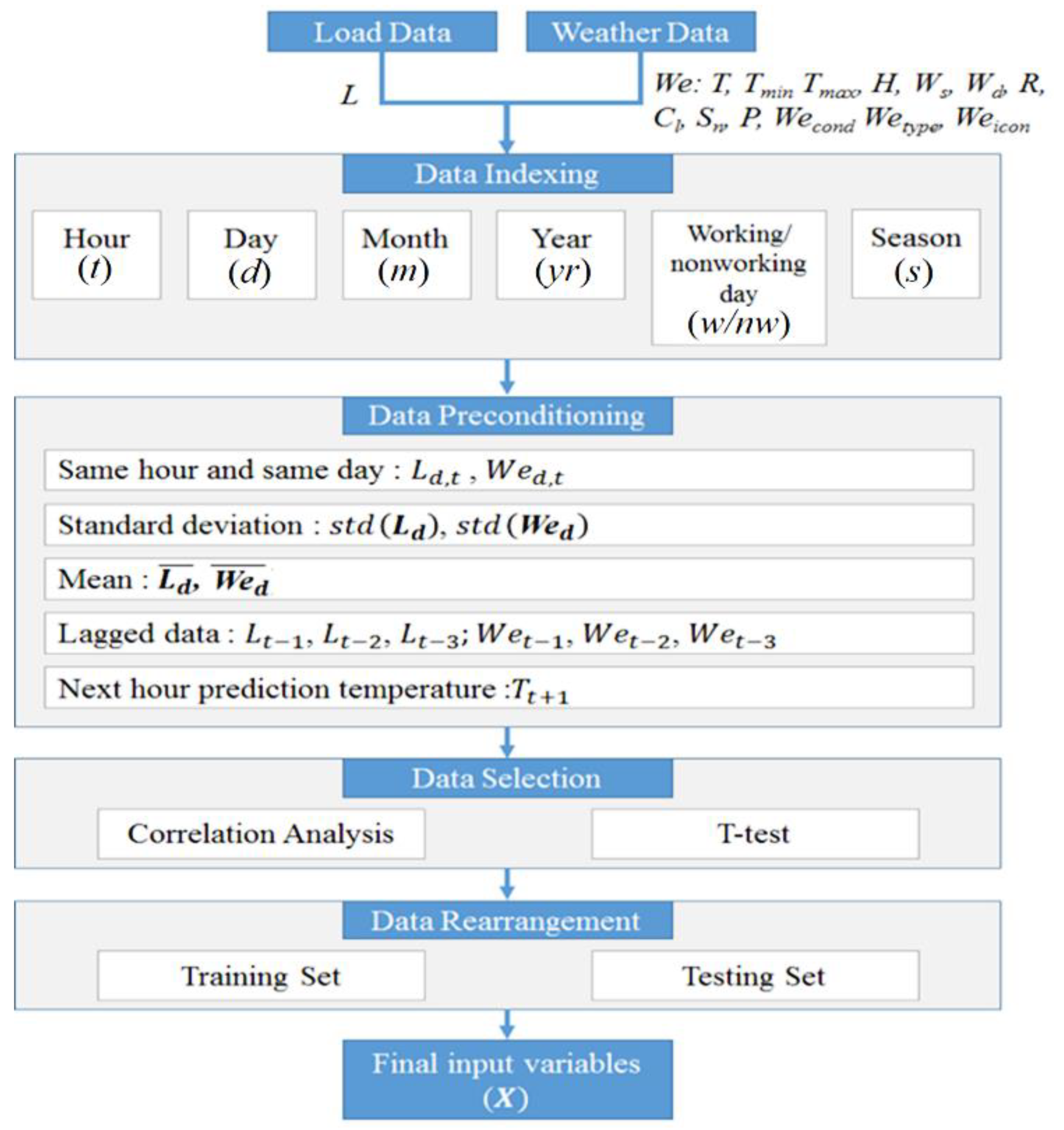
Appropriate selection of input variables based on historical load and weather variables that affect load pattern is essential for STLF. Xin et al. [20] use correlation analysis to choose the decomposed signal. In this paper, the correlation analysis is utilized to select proper input variables from several preconditioned data. As shown in Figure 1, for selection of the input variables, historical data is modeled through the following steps, which are the data indexing, data preconditioning, data selection, and data rearrangement.

As the initial step, load data and weather information are prepared based on [21,22], respectively. The data are arranged as a column-vector sorted in the row sequence. The input data for both system- and end-user load are hourly data. The historical load (L) data are in metric of kW. The historical weather data (We) consist of temperature (T), maximum temperature (T_max), minimum temperature (T_min), humidity (H), wind speed (W_s), wind direction (W_d), rain (R), cloud (C_l), snow (S_n), pressure (P), weather condition (We_cond), weather type (We_type), and weather icon (We_icon).

We_cond, We_type, and We_icon above are the weather information summary within the observed hour. We_cond describes the general weather conditions, varying from clouds, rain, smoke, thunderstorm, drizzle, haze, and mist. We_type gives a detailed description of each We_cond, such as scattered clouds, few clouds, broken clouds, proximity shower rain, thunderstorm with light rain, light-intensity shower rain, light rain, light-intensity drizzle, and mist. We_icon is the visualization code of We_type and We_cond. Detailed information about the weather can be found in [22].

In the next step, the following inputs are indexed into six different labels according to the hour (t), day (d), month (m), year (yr), working/non-working day (w/nw), and season (s). This process is done to ease the later process in the data preconditioning. Using this index, we can easily rearrange the data into several preconditions that may have strong relations to the predicted signal. Weather information and calendar events are also mapped to a load pattern to explain feature correlation.

Then, the load and weather data are manipulated into several conditions in the data preconditioning step. The same hour and same day, daily mean and standard deviation, lagged data, and next-hour prediction temperature are chosen. The lagged data, up to the previous three hours, are used to avoid misinterpretation of non-stationary load patterns. The lagged version of the load data allows the prediction model to include the recent history of a load sequence. For example, load in hour-24 is highly correlated with the load variation between hour-21 and hour-23. By using the lagged data, the sequential load variation pattern can thus be captured.

After the data preconditioning is done, the data selection and data rearrangement are processed. From the following series, the correlation analysis and t-test are used to achieve the input-output relation and relationship strength between each input to the output. Based on the result of t-test, the input vectors that have p-value lower than 0.05 are classified as significant and used as input variables. Then, the selected vectors are classified into the tuning set and testing set with ratios of 70% and 30%, respectively, to the length of total historical data. The final input variables are then constructed.

3. Proposed Prediction Method

In general, a load pattern is the result of aggregated user behaviors from a downstream level to a high-voltage level, in which the pattern repetition is affected in accordance to the level of aggregation. The wider the system region, the lower non-stationary part of the load pattern is than the narrow system region because the associated weather or user-behavior changes are canceled out by each other. The difficulties in the STLF lie on the precision of modeling different load characteristics, especially from system-side to aggregate end-user load data. DWT has been used to model various load characteristics with different wavelet types and decomposition levels, as previously investigated in [11,12,13,14,15,16]. However, the best reconstruction of DWT remained unsolved. 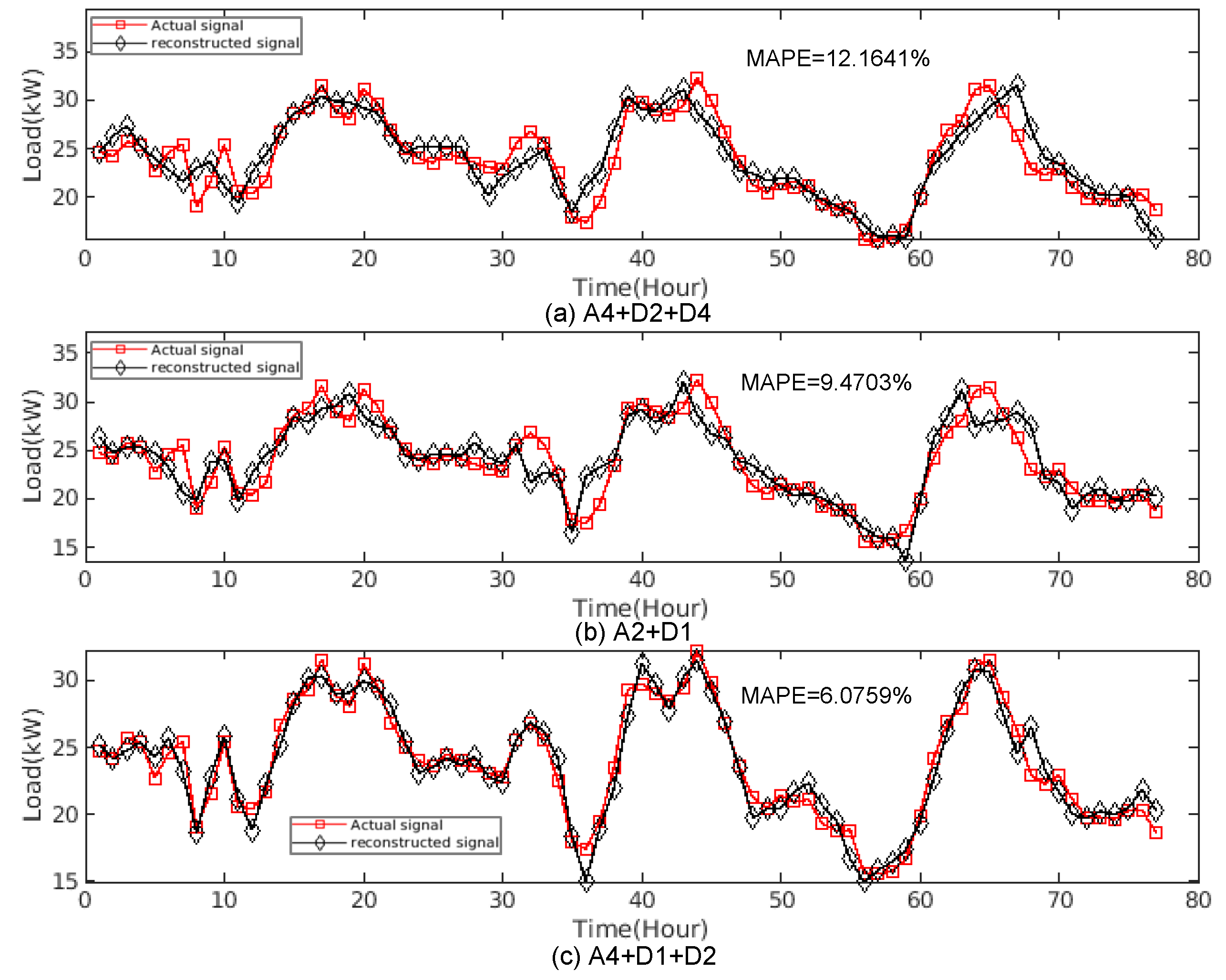Figure 2 shows the forecasting results of different reconstructions of DWT using Db2. The figure shows that the forecasting accuracy varies by different combinations of approximation and detail components (A_m + D_m). In Figure 2a, the signal is reconstructed from approximation level-4 and detail components level-2 and level-4, which are shortened as A4, D2, and D4, respectively. Similarly, the combination of A2 and D1 and combination of A4, D1, and D2 are used for Figure 2b,c, respectively. As seen from Figure 2a,c, though they use same level of decomposition with different combination of detail components, the MAPE changes drastically. Besides, in Figure 2b, by only using approximation and detail component in decomposition level-2, it may achieve 9.4703% of MAPE, which is lower than the MAPE in Figure 2a that uses decomposition level-4. It reflects that, unique to each signal, the chosen set of approximation and detail components affects the decomposed signals and accuracy of prediction. The reconstruction by using decomposed signals may either fit to the original load pattern or distort the original signal. Therefore, the best reconstruction by using decomposed signals is an important task in modeling historical data and prediction.

3.1. The Proposed WOA-DWT-MLR Method

In this paper, the term of “open-ended” defines the general functionality of the prediction method which is flexible in the application of system and end-user sides. An open-ended prediction method is expected to have the capability to accommodate different load characteristics of aggregated system load and individual end-user load, which have majorly different load characteristics observed from their signal waveform and load capacity. The characteristic of system load is steadier in variation than end-user load because the changes of aggregated load from various feeders are canceled out by each other and result in less fluctuation.

Differing from the system load, the end-user load fluctuates much more according to the local weather, user behavior, calendar, and usage of appliances. Those factors complicate the variation and randomness of the load pattern from hour to hours and day to days. An open-ended prediction method is expected to always have the best performance without any site-specific constraint, a fact which is possible to be achieved by setting the optimal prediction model from the chosen inputs.

The open-ended prediction method is formulated based on WOA-DWT-MLR model. WOA is used to find the optimal level of decomposition, type of wavelet, and composition of details and approximations before those sub-signals are modeled into several MLR models. The DWT decomposes the non-stationary part of inputs into several high- and low- frequency components and reconstructs them in the original time domain signal. DWT uses the Daubechies type of wavelet which has scale and translation parameters for transforming the signal into low- and high-frequency coefficients. The low-frequency sub-signal is called as approximation component, while the high frequency part is called as detail component. Search space of the Daubechies can be formulated as:

$$DW{T}_{r,m}\left(n\right)=\frac{1}{\sqrt{2^r}}\psi \left(\frac{1}{2^r}\left(n-2^{r}m\right)\right),$$

(1)

where r is DWT’s level of resolution, and m is scale parameter relating to time step n. DWT is tuned to find appropriate values in the wavelet type and decomposition level. The trend of the signal is coarsened by the approximation component. The high frequency of the signal is captured by the detail component. When the decomposition level is increased, the density of signal variation decreases or sparser. For further details, refer to Mallat [23].

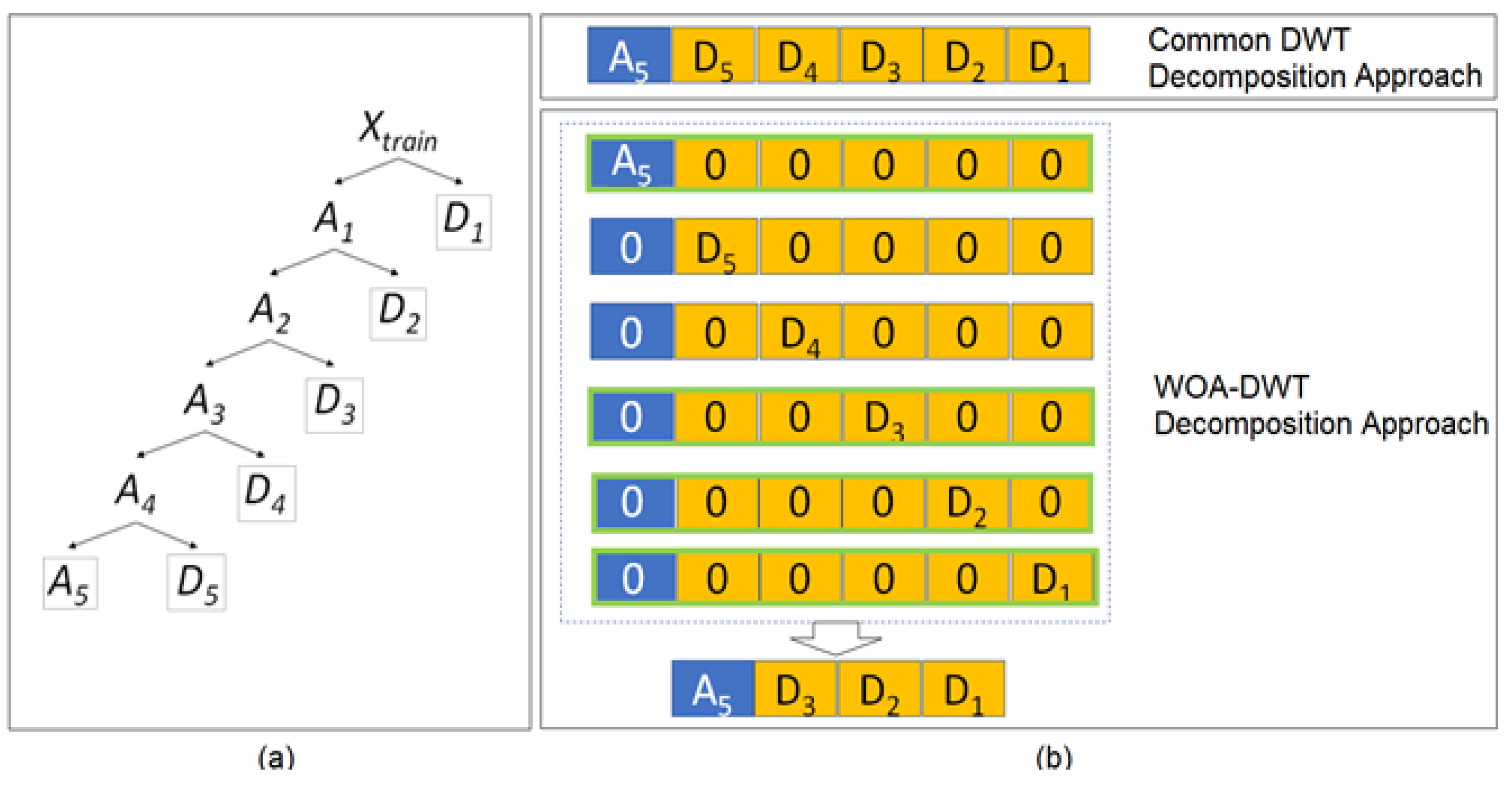
Figure 3 shows the DWT modeling process in the proposed WOA-DWT-MLR. Figure 3a shows the decomposition tree of the proposed WOA-DWT-MLR, setting level-5 as the maximal level for the WOA-DWT. In the proposed decomposition approach, the signal is independently decomposed to the set of Daubechies levels and types by handling the selected decomposition coefficients while the remaining coefficients are replaced with zero. Based on this scheme, the signal can be extracted to its unique characteristics reflected by individual approximation and detail components. Instead of taking the common decomposition structure as [A_r, D_r, …, D₁], WOA is utilized to find the optimal combination of the decomposed parts. This approach is taken to sort out the less necessary DWT components to achieve accurate reconstruction of the actual signal. Only the selected parts of decomposition are reconstructed. Figure 3b shows the illustration with the proposed method having [A₅, D₃, D₂, D₁] as the final combination, due to less Least Square Error (LSE), as in Equation (12), than the common structure of [A₅, D₅, D₄, D₃, D₂, D₁].

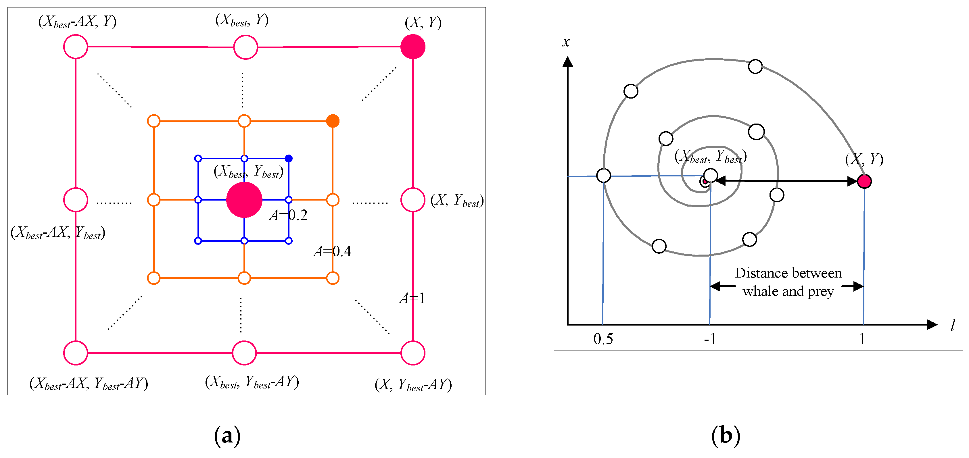
According to Mirjalili and Lewis [19], a humpback whale attacks prey by adopting the bubble-net feeding strategy. Figure 4 shows this strategy with its shrinking encircling mechanism and spiral updating process as used in the WOA [19]. The bubble-net feeding strategy is the hunting method of whales by creating some bubbles along a spiral to corner the prey close to the surface before eating them. In the mathematical model as illustrated in Figure 4a, the bubble tags are modeled as position from (X, Y) towards (X_best, Y_best), following a vector coefficient of 0 ≤ A ≤ 1, to replicate the shrinking spiral of a whale to corner the prey. As shown in Figure 4b, the spiral position updating process is used to update the distance between the whale located at (X, Y) and the prey located at (X_best, Y_best). The whale corners the prey within the shrinking circle and spiral shape, simultaneously, through random update of position (X, Y) toward (X_best, Y_best). In the optimization algorithm, WOA optimizes the solutions following the number of search agents to tune the best performance. Basically, WOA calculates the location of bubbles as the solutions and encircles them in the n-dimension search space. In this research, WOA finds the set of approximation and detail components that has the minimum LSE as the objective function in the tuning stage. Search agents then move in a hyper-cubed way around the current best solution. The position of a search agent can be updated according to the position of the current best record X_best. Different places around the best agent can be achieved with respect to the current position by adjusting the value of coefficient vectors $\overrightarrow{A}$ and $\overrightarrow{C}$.

The updating process of current position is written as follows:

$$\overrightarrow{D}=\left|\overrightarrow{C}·{\stackrel{\rightharpoonup }{X}}_{best}\left(iter\right)-\overrightarrow{X}\right|,$$

(2)

$$\overrightarrow{X}\left(iter+1\right)={\overrightarrow{X}}_{best}\left(iter\right)-\overrightarrow{A}·\overrightarrow{D},$$

(3)

$$\overrightarrow{A}=2\overrightarrow{a}·\overrightarrow{r}-\overrightarrow{a},$$

(4)

$$\overrightarrow{C}=2·\overrightarrow{r},$$

(5)

where iter indicates the current iteration, ${\stackrel{\rightharpoonup }{X}}_{best}$ and $\overrightarrow{X}$ are the latest position vector of the best solution obtained and position vector, respectively, and $\overrightarrow{a}$ describes the shrinking bubble-net strategy to the surface by linearly decreased from 2 to 0 over the course of iterations, while $\overrightarrow{r}$ is a random vector in [0, 1]. The humpback whales swim around the prey within a shrinking circle and along a spiral-shaped path simultaneously. There are two approaches to search for prey in WOA, which are exploitation and exploration. The exploitation phase uses the bubble-net attacking method, following the shrinking encircling mechanism and spiral updating position, which assumes 50% probability as follows:

$$\overrightarrow{X}\left(iter+1\right)=\{\begin{array}{c}{\stackrel{\rightharpoonup }{X}}_{best}\left(iter\right)-\overrightarrow{A}·\overrightarrow{D}, if p<0.5\\ \overrightarrow{D^{\prime }}·e^{bl}·\cos \left(2\pi l\right)+{\stackrel{\rightharpoonup }{X}}_{best}\left(iter\right), if p\ge 0.5\end{array}.$$

(6)

• Shrinking encircling mechanism: this behavior is modeled by decreasing the value of $\overrightarrow{a}$ in Equation (4) and further use $\overrightarrow{A}$ in Equation (6) with p < 0.5. $\overrightarrow{A}$ is a random value in the interval of [−a, a], where a is decreased from 2 to 0 over the iterations.
• Spiral updating position: this approach initially calculates the distance between the whale location X and prey location $X_{best}$ and then constructs a spiral equation between the X and and $X_{best}$ to mimic the helix-shaped movement of humpback whales as Equation (6) with p ≥ 0.5, where $\overrightarrow{D^{\prime }}=\left|{\stackrel{\rightharpoonup }{X}}_{best}\left(iter\right)-\overrightarrow{X}\left(iter\right)\right|$ indicates the distance of the ith whale to the current best solution. In this approach, b is a constant describing the shape of the logarithmic spiral, while l is a random number in [−1, 1].

The exploration of the humpback whales is defined by a random search with coefficient vector $\left|\overrightarrow{A}\right|>1$ that allows WOA to perform a global search. Instead of using the current best agent, the humpback whales choose the search agent randomly based on the position of each other. This mechanism can be modeled as follows:

$$\overrightarrow{D}=\left|\overrightarrow{C}·{\stackrel{\rightharpoonup }{X}}_{rand}-\overrightarrow{X}\right|,$$

(7)

$$\overrightarrow{X}\left(iter+1\right)={\stackrel{\rightharpoonup }{X}}_{rand}-\overrightarrow{A}·\overrightarrow{D},$$

(8)

where ${\stackrel{\rightharpoonup }{X}}_{rand}$ is a random position vector (a random whale) chosen from the current population.

In the proposed method, the search vectors of WOA are the wavelet type $so{l}_{i,1}$, decomposition level $so{l}_{i,2}$, and reconstruction of details and approximation being used $so{l}_{i,3}$. These search vectors are accommodated in $\overrightarrow{X}$, which is then extended to the size of agent numbers and search vectors as row and column, respectively. After several iterations, the set of solutions is fed to DWT to get the optimal approximation-component $a_k$ and detail-components $d_k$ varying from k = 1, 2, 3, …, $so{l}_{i,2}$ that achieve minimum prediction error. Then, the final decomposition sub-signals of WOA-DWT are used in prediction model, following the multiple linear regression model as in Equation (9):

$$y_i=\alpha +{\beta }_1{x}_{i1}+{\beta }_2{x}_{i2}+\cdots +{\beta }_k{x}_{ik}+e_i ,$$

(9)

$$y_{out}= y_{i\_a_k}+\cdots +y_{i_{d_k}}, LS{E}_{y_{out}}=\min \left(LSE\right).$$

(10)

The final prediction output is the summation of best combination MLR model that has the minimum LSE as in Equation (10). The prediction output of each Daubechies wavelet component y_i is calculated from the input variables X, regression coefficients β, intercept α, and observed model error e. The intercept α and regression coefficient β are obtained using the least-square estimator that minimizes the sum of square errors (residuals).

$$S={{\displaystyle \sum }}^{}{ϵ}_t{}^2={{\displaystyle \sum }}^{}{\left(Y_t-{\widehat{Y}}_t\right)}^2,$$

(11)

where ${ϵ}_t$ is residual error between actual $Y_t$ and prediction value ${\widehat{Y}}_t$ at observed hour t.

The proposed prediction model is evaluated by LSE and Mean Absolute Percentage Error (MAPE). LSE evaluates the WOA optimization, while MAPE evaluates absolute error between the prediction result and actual load data. Calculation of MAPE and LSE based on number of hours Nh is shown in Equations (12) and (13) as follows:

$$LSE=\frac{1}{Nh}{{\displaystyle \sum }}_{t=1}^{Nh}{\left|Y_t-{\widehat{Y}}_t\right|}^2,$$

(12)

$$MAPE=\frac{1}{Nh}{{\displaystyle \sum }}_{t=1}^{Nh}\left|\frac{Y_t-{\widehat{Y}}_t}{Y_t}\right|\times 100\%.$$

(13)

3.2. Prediction Models of Tuning and Testing Stages

Tuning, validation, and testing stages are run to build the prediction models. Figure 5a,b shows the tuning and testing stages, respectively, of the proposed WOA-DWT-MLR to find the best prediction model. In the proposed method, the DWT is subjected to each data set to handle the unique periodicity of those seasons. DWT with the initial parameter tuned by WOA calculates the decomposition layer of a set of input and output data. The initial parameter is taken randomly between 2 to 5 for Daubechies level r and 1 to 5 for Daubechies type m. The validation stage is performed as the preliminary testing after prediction model is built in the tuning stage. Each of these reconstructed signals is utilized in several individual MLR models. The output of each MLR is summed and the LSE is calculated. The best prediction model with the minimum LSE is chosen as the final prediction model after several iterations. In the tuning process, validation will be conducted using last 24-h time series data in each season. In the testing stage, the tuned prediction model is tested with the testing data set. The tuning stage takes 70% of the data to get more insight of the daily pattern. Both validation and testing stages use the remaining 15% of data.

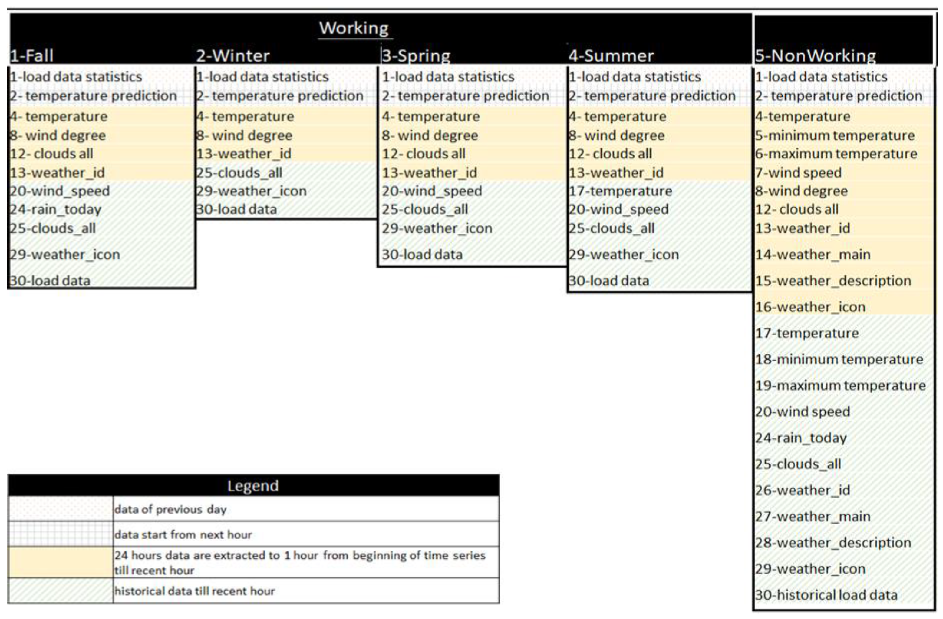
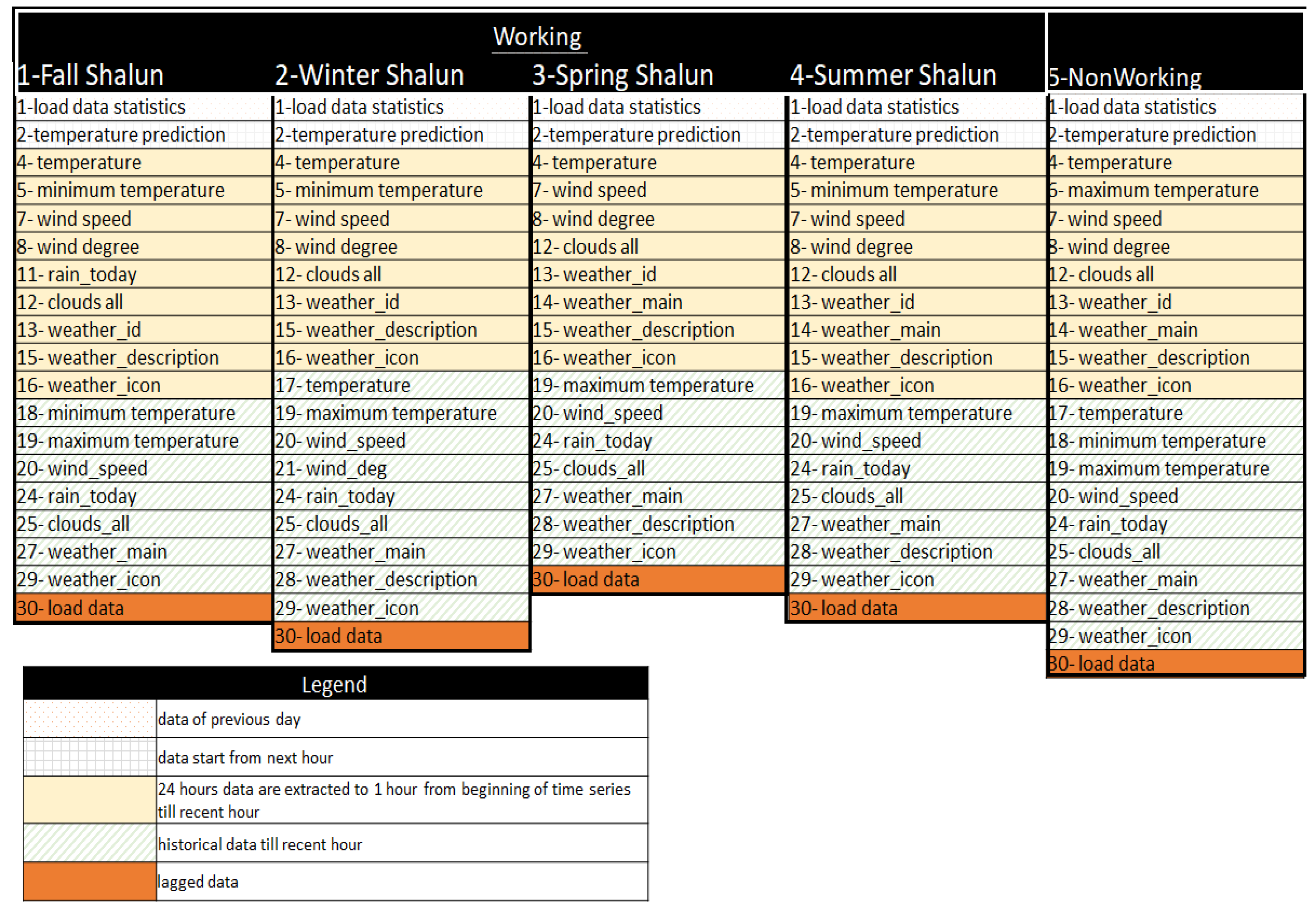
To show the effectiveness of the proposed prediction model, the inputs for both system and end-user data sets are differentiated into working day and non-working day models. In the working day model, historical data from Monday to Friday is contained, including deferred holidays to compensate for holidays that fall on weekends. The data set excludes holiday happening within these days. The non-working day model covers Saturday to Sunday, including national holidays happening on weekdays.

The proposed method is tested by the system data set and end-user data set. In the system data set, there are four different season models, starting from Fall, Winter, Spring, and Summer. It is assumed that Fall runs from September to November, and so on for the remaining season models in different months. For the end-user data set, there are only two different season models which are sets of Fall-Winter and Spring-Summer, respectively. The Fall-Winter model is assumed to begin at September and last till February. The end-user data set consists of only two different unique models because of data lacking issues.

3.3. Benchmark Algorithms

To validate performance of the proposed method, five well-known algorithms are used as benchmark. These methods have been applied to the same day-ahead load forecasting to show individual prominent results. The comparison methods are traditional MLR, ANN, Autoregressive moving average with exogenous input (ARMAX), support vector regression (SVR), and PSO-DWT-MLR. Brief descriptions about the algorithms are as follows:

• MLR (Mohammad et al. [24]): the MLR prediction model calculates the targeted output based on a set of predictors in which the coefficients of each predictor are calculated by least sum of squares as in Equation (9). For the validation of the proposed method, MLR uses the same input variables as the proposed method.
• ANN (Hernández et al. [25]): the ANN consists of the input layer, hidden layers, and output layer interconnected via weights between nodes or neurons. To get the best weights from regression models that describe the relationship between input variables and next-day hourly prediction, the number of ANN’s hidden neurons needs to be fine-tuned.
• ARMAX (Hong-Tzer et al. [26]): ARMAX is used to model the relationship between load demand and exogenous input variables. The ARMAX model can be written as follows:

  $$A\left(q\right)y\left(t\right)=B\left(q\right)u\left(t-nk\right)+C\left(q\right)e\left(t\right),$$

  (14)

  where y(t) is the load demand, u(t) is the exogenous input related to load demand, e(t) is white noise, and q⁻¹ is a back-shift operator. $A\left(q\right)=1+a_1{q}^{-1}+\cdots +a_{na}{q}^{-na}, a_1,\dots , a_{na}$ are parameters of the Autoregressive (AR) part, na is the AR order; $B\left(q\right)=b_1+b_1{q}^{-1}+\cdots +a_{nb}{q}^{-nb+1}, b_1,\dots , b_{nb}$ are parameters of the exogenous input (X) part, nb is the input order; $C\left(q\right)=1+c_1{q}^{-1}+\cdots +c_{nc}{q}^{-nc}, c_1,\dots , c_{nc}$ are parameters of the Moving Average (MA) part, and nc is the MA order. To get the best tune of ARMAX parameters, PSO is used for each data set.
• SVR (Cortez and Vapnik [27], Chen et al. [28]): SVR is a non-parametric technique using sequential minimal optimization to solve a decomposed equation for the input variables. For each iteration, a working set of two points is chosen to find a function f(x) that deviates from y_n by the value not greater than the error in each previous training point of x. The result of iteration process can be recalled as the mapping of the training data x into high dimensional feature space to represent nonlinear relationship between input variables and targeted output.
• PSO-DWT-MLR: the prediction method uses PSO (Zhan et al. [29]) as the optimization algorithm to find the best combination of reconstructed signals. PSO is used to optimize the DWT type, level, and combination of wavelet component, as WOA did in the proposed method.

4. Simulation Results

The proposed method is simulated in MATLAB 2018 environment running with Intel Core™ i-73770 CPU of 3.40 GHz and 8 GB RAM. The decomposition level of DWT tuned by WOA is between level-2 and level-5, while the type of DWT is between Db1 to Db5. The search agent of WOA is set to 50 with three solutions for decomposition level, type of wavelet, and combination between reconstruction of details and approximation being used. WOA is also set with 50 iterations maximum to find the optimal solution. For each tuning model, best performance and error distribution are observed in ten trials. The performance is analyzed with MAPE in the validation stage and testing stage. The prediction results of traditional MLR, ANN [25], autoregressive moving average with exogenous input (ARMAX) [26], support vector regression (SVR) [27,28], and PSO-DWT-MLR are also provided to show the effectiveness of proposed WOA-DWT-MLR. In MLR, optimal coefficients are found by least square error. ANN uses six and seven hidden neurons in the single hidden layer for working day model and non-working day model, respectively. ARMAX uses optimal order tuned by PSO where the lagged time series and exogenous inputs are modeled as Gaussian distribution. SVR is set with Sequential Minimal Optimization (SMO) solver. Besides, PSO-DWT-MLR is used to compare the effectiveness of WOA over PSO. All methods use the same input/output data sets for tuning, validation, and testing. The existing methods are fine-tuned uniquely according to each data set.

4.1. Test System

The proposed method was tested on two different data sets that represent the system and end-user data sets. The system data set used Independent System Operator of New England (ISO-NE). ISO-NE is the regional transmission organization (RTO) that serves six regions with headquarters in Massachusetts. The data can be accessed in [21]. Two years of data, from 1 January 2016 to 31 December 2017, was used. The end-user data set used load demand of Green Energy Building located in Shalun Campus of National Cheng Kung University. The end-user data set consisted of aggregation of three different smart meters in which the data set from 17 May 2017 to 26 September 2018 was taken for the simulation.

The weather data used in this paper was taken from open access weather data provider as Application Programming Interface (API) in [22], which presents information about temperature, humidity, wind speed, wind gust, cloud condition, weather condition, and weather icon. Data, such as temperature which may vary from positive to negative (for four-season countries), is preconditioned in Kelvin metric instead of using Celsius. For condition explanation, such as “cloudy”, “sunny”, “partly showered”, and so on, the weather-explanation is converted into the unique discrete range.

As explained in historical data modeling approach shown in Figure 1, the input variables are selected with high correlated parameters using the correlation analysis and t-test. The results of correlation analysis and t-test are shown in

Table 1. Correlation analysis and T-test of input variables.

Name	R	p-Value	Correlated (1)/Non Correlated (0)
Minimum temperature	5.100 $\times {10}^{-2}$	9.131 $\times {10}^{-21}$	1
Maximum temperature	3.627 $\times {10}^{-2}$	3.052 $\times {10}^{-11}$	1
Pressure	−8.197 $\times {10}^{-3}$	1.333 $\times {10}^{-1}$	0
Humidity	−5.185 $\times {10}^{-3}$	3.424 $\times {10}^{-1}$	0
Wind speed	−4.580 $\times {10}^{-2}$	4.816 $\times {10}^{-17}$	1
Wind degree	1.365 $\times {10}^{-2}$	1.246 $\times {10}^{-2}$	1
Rain 1 h	1.880 $\times {10}^{-2}$	5.738 $\times {10}^{-4}$	1
Rain 3 h	3.168 $\times {10}^{-2}$	6.533 $\times {10}^{-9}$	1
Rain 24 h	9.255$\times {10}^{-3}$	9.012 $\times {10}^{-2}$	0
Rain today	1.989 $\times {10}^{-2}$	2.707 $\times {10}^{-4}$	1
Snow 1 h	−3.963 $\times {10}^{-3}$	4.680 $\times {10}^{-1}$	0
Clouds all	−3.889 $\times {10}^{-2}$	1.040 $\times {10}^{-12}$	1
Weather ID	2.118 $\times {10}^{-2}$	1.050 $\times {10}^{-4}$	1
Weather main	−2.779 $\times {10}^{-2}$	3.594 $\times {10}^{-7}$	1
Weather description	−4.250 $\times {10}^{-2}$	6.884 $\times {10}^{-15}$	1
Weather icon	−2.552 $\times {10}^{-2}$	2.952 $\times {10}^{-6}$	1

. Then, these parameters are given to WOA-DWT-MLR to get the coefficient β of each input variable from the chosen DWT components. In the training stage, we can figure out that each season (Fall, Winter, Spring, and Summer) has a unique combination of coefficients which consist of nonzero values and zeros. The observation results of Fall in the working day of the ISO-NE data set are shown in Figure 6. The data set of Fall is labeled as 1-Fall, which consists of approximation component level-4 and detail components level-1, 2, and 3, which are shortened as A4, D1, D2, and D3, respectively. We can infer that the nonzero coefficients reflect the relation of the input variables to the targeted output, while the zero coefficients reflect that it has no relation to the targeted output, though it is already chosen from correlation analysis and t-test.

The selected input variables used for each season in working and non-working data sets are listed in Figure 7 and Figure 8 for the ISO-NE data set and the Shalun data set, respectively. From these figures, the ISO-NE test system is less sensitive to the lagged data as the selected input variable of predictors in the Shalun test system. We can infer that the lagged data are not a strong correlated predictor to the prediction result in the ISO-NE data set. The sensitivity above is measured by observing the zero and nonzero values in the MLR coefficients. Besides, the ISO-NE test system needs less weather information than the Shalun test system. For both test systems, each season in the non-working data set has similar input variables, owing to the effect of data scarcity in comparison to the working data set.

4.2. Numerical Results

The best WOA-DWT-MLR prediction model obtained can be observed in

Table 2. Best prediction model of ISO-NE data set.

Season	Wav. Type	Dec. Level	Wavelet Reconstruction	Day Type
Fall	Db3	4	A4, D1, D2, D3,	Working
Winter	Db3	4	A4, D1, D2, D3,
Spring	Db5	5	A5, D1, D2, D3, D4, D5
Summer	Db5	5	A5, D1, D2, D3, D4, D5
Fall	Db5	4	A4, D1, D2, D3, D4, D5	Non-working
Winter	Db4	5	A5, D1, D2, D3, D4
Spring	Db3	4	A4, D1, D2
Summer	Db5	5	A5, D2, D3, D4

and

Table 3. Best prediction model of End-User data set.

Season	Wav. Type	Dec. Level	Wavelet Reconstruction	Day Type
Fall-Winter	Db3	3	A3, D1, D2, D3	Working
Spring-Summer	Db5	5	A5, D1, D2, D3, D4, D5
Fall-Winter	Db3	3	A3, D2, D3	Non-working
Spring-Summer	Db4	4	A4, D1, D2, D3, D4

. Prediction models of working and non-working days for the system data set are shown in Table 2. It is observed that the best decomposition of level-4 and level-5 is obtained with wavelet types Db3, Db4, and Db5. For the end-user data set, the prediction models are shown in Table 3. In the end-user data set, the best prediction model uses decomposition level-3, level-4, and level-5 with wavelet types of Db3, Db4, and Db5.

4.2.1. ISO-NE Data Set

Prediction results of the system data set (ISO-NE) are shown in

Table 4. Prediction results of ISO-NE (working day). ANN = artificial neural network; PSO = particle swarm optimization; ARMAX = Autoregressive moving average with exogenous input; SVR = support vector regression.

Validation Error (%)	Fall	Winter	Spring	Summer
MLR	1.8383	1.8793	2.0956	1.4659
ANN	2.5472	2.1815	2.3387	1.4975
ARMAX	4.1761	2.0931	4.7462	2.3154
SVR	2.1130	1.8543	1.9406	2.3740
PSO-DWT-MLR	1.1963	1.2122	1.2380	1.3043
WOA-DWT-MLR	1.1487	1.0603	1.0414	0.8322
Testing Error (%)	Fall	Winter	Spring	Summer
MLR	1.8161	3.8908	1.9223	1.9868
ANN	2.1125	2.9227	2.1748	2.0401
ARMAX	4.4960	2.4762	4.5653	2.4149
SVR	2.32740	1.95772	1.96806	5.19816
PSO-DWT-MLR	1.3860	2.3867	1.3348	1.8368
WOA-DWT-MLR	1.3024	1.6928	1.0104	0.9213

for working days. In the validation stage, the proposed method achieves 1.1487%, 1.0603%, 1.0414%, and 0.8322% MAPE in Fall, Winter, Spring, and Summer, respectively. When the final prediction model is tested, the proposed method further shows its significant improvements among other methods by leading the accuracy with 1.3024%, 1.6928%, 1.0104%, and 0.9213% MAPE. If validation errors are compared head-to-head to testing errors among four seasons, prediction models of the proposed method can hold their accuracy with MAPE of 0.1537%, 0.6325%, 0.031%, and 0.0909%, respectively, as compared to PSO-DWT-MLR.

For non-working data set, the proposed method also surpasses the compared methods in validation stage with 1.2781%, 1.0374%, 1.3055%, and 1.4311% for Fall, Winter, Spring, and Summer, respectively, as listed in

Table 5. Prediction results of ISO-NE (non-working day).

Validation Error (%)	Fall	Winter	Spring	Summer
MLR	1.9704	1.8694	2.2309	2.2502
ANN	3.1560	1.8876	2.9832	3.5523
ARMAX	2.3650	2.2913	3.4135	7.2335
SVR	1.8625	1.8376	2.0260	2.0172
PSO-DWT-MLR	1.8375	1.5342	1.4269	1.5848
WOA-DWT-MLR	1.2781	1.0374	1.3055	1.4311
Testing Error (%)	Fall	Winter	Spring	Summer
MLR	2.3733	2.1621	1.6637	2.1986
ANN	3.3239	2.2801	2.7051	3.1254
ARMAX	2.7512	2.8100	3.3978	7.0049
SVR	2.3201	2.1227	1.5502	2.1961
PSO-DWT-MLR	2.0463	2.0789	1.3616	1.2338
WOA-DWT-MLR	1.5869	1.2811	1.3399	1.2398

. Though the same data set was applied to all methods, the ARMAX model fails to hold its prediction consistency in Summer, due to its inability in coefficient determination when load variation is high as the effect of less data and unexpected weather variations. The proposed method can have the lowest MAPE of 1.5869%, 1.2811%, 1.3399%, and 1.2398% for Fall to Summer in the testing stage.

The predicted load patterns for the system data set in working day are observed in Figure 9a. ARMAX faces difficulty in being consistent when the actual load pattern changes drastically in transition of working hour to lunch time and transition of working hour to dinner time (as shown from hour-10 to hour-13 and hour-16 to hour-19), while the other non-parametric based methods, such as the proposed method, can predict the actual load pattern better. In this figure, MLR can closely predict the load variation because the preconditioned input variables cover the detail associated weather and statistical load data for standard deviation and mean value. Furthermore, in Figure 9b, compared methods cannot closely predict the actual load on the valley-like pattern nor transition to a peak load, as shown between hour-5 and hour-15. In contrast, the proposed method can predict the actual load well, while other methods still have a significant gap to the actual load.

4.2.2. End-User Data Set

For the end-user data set, load variation is expected to happen in the actual load signal, due to the aggregation of only three smart meters. The variation is strongly related to any human behavior inside the offices. For the working data set, the proposed method successfully presides at the prediction accuracy of 5.4697% and 3.2479% as compared to the other methods which have almost twice and higher MAPE in validation stage, as shown in

Table 6. Prediction result of Shalun (working day).

Validation Error (%)	Fall-Winter	Spring-Summer
MLR	15.0677	7.1133
ANN	19.9037	7.9612
ARMAX	10.4263	10.6182
SVR	13.5051	6.8966
PSO-DWT-MLR	5.6531	3.4675
WOA-DWT-MLR	5.4697	3.2479
Testing Error (%)	Fall-Winter	Spring-Summer
MLR	9.3383	13.3464
ANN	10.5189	20.3770
ARMAX	9.6939	13.3079
SVR	8.6685	12.8394
PSO-DWT-MLR	6.1665	5.5546
WOA-DWT-MLR	6.0246	5.5222

. Differing from other non-parametric and traditional regression methods, PSO-DWT-MLR provides the second accurate prediction. This is the proof that the integration of signal decomposition improves the prediction accuracy. In the testing stage, the proposed method can hold its prediction consistency by surpassing the other methods with 6.0246% and 5.5222% of MAPE. The prediction performance of Spring-Summer model in testing stage decreases in the validation stage because the data in the testing stage contains many missing data.

Table 7. Prediction result of Shalun (non-working day).

Validation Error (%)	Fall-Winter	Spring-Summer
MLR	9.6415	17.4223
ANN	12.8374	17.6259
ARMAX	21.5325	10.5514
SVR	8.3827	16.0362
PSO-DWT-MLR	6.9836	8.6637
WOA-DWT-MLR	5.3888	3.2748
Testing Error (%)	Fall-Winter	Spring-Summer
MLR	8.5347	14.1043
ANN	9.8549	14.8972
ARMAX	21.2365	11.5149
SVR	8.0799	10.9618
PSO-DWT-MLR	6.1767	9.2912
WOA-DWT-MLR	6.1767	9.2912

presents prediction accuracy of the non-working data set. The proposed method outperforms the other methods with 5.3888% and 3.2748% MAPE in validation stage for the Fall–Winter model and Spring-Summer model, respectively, and maintains the corresponding testing errors of 6.1767% and 9.2912% MAPE. Non-consistent performance of MLR, ANN, ARMAX, and SVR is shown, even though the testing error is less than the validation error.

Performance of different prediction models is analyzed from the load patterns in Figure 10a,b for working and non-working days, respectively. In Figure 10a, both the proposed method and PSO-DWT-MLR outperform the other comparison methods. In Figure 10b, ANN and ARMAX fail to fit the prediction results to actual load. The MLR-based prediction model fits the actual load, but only the proposed method has the best performance among the compared methods.

5. Discussion

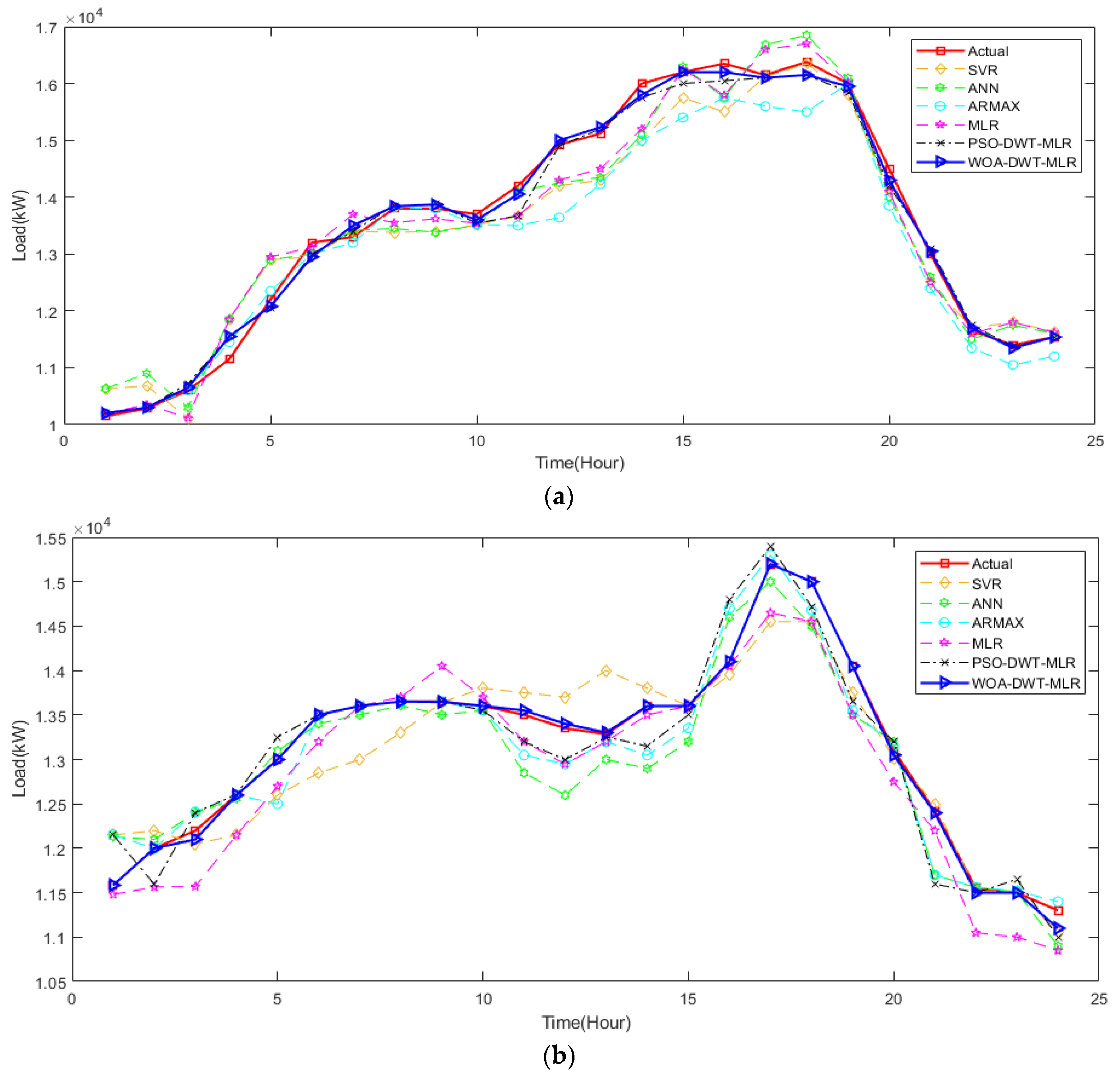
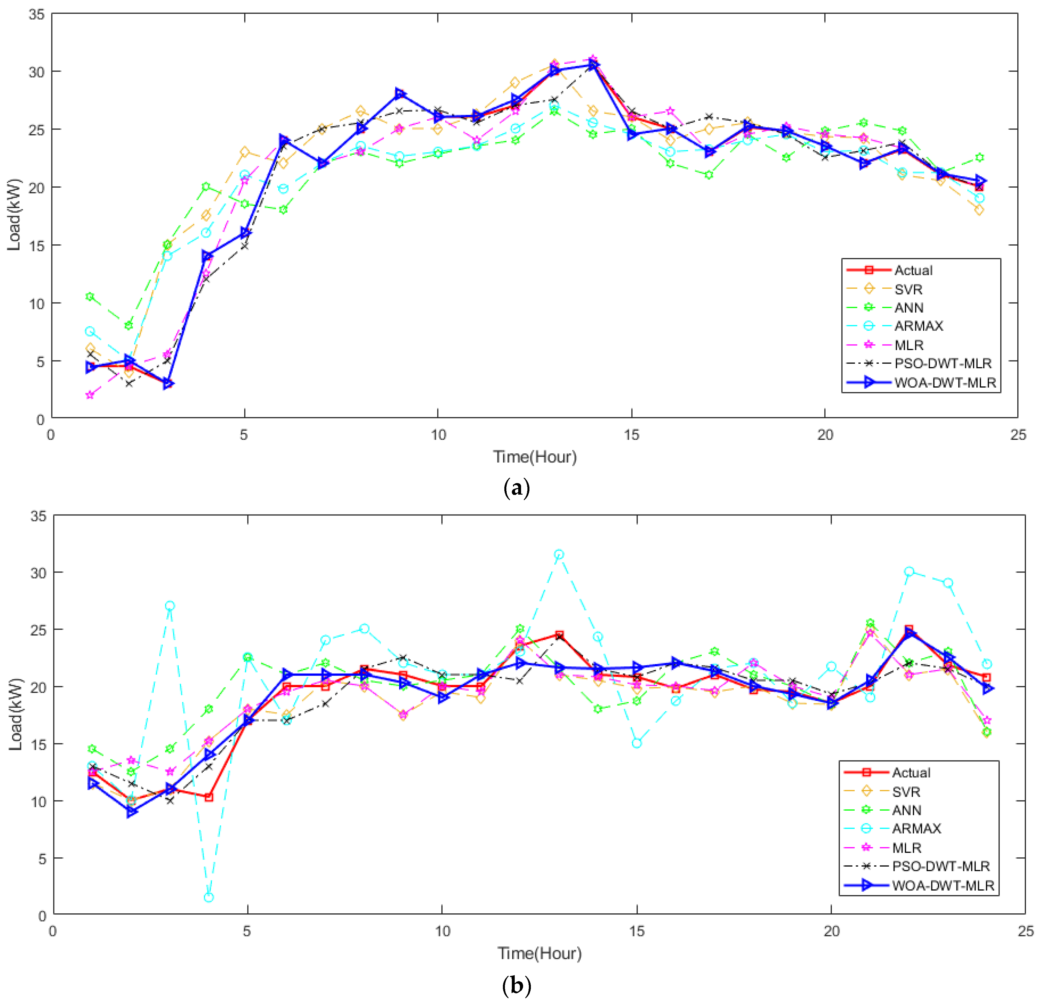
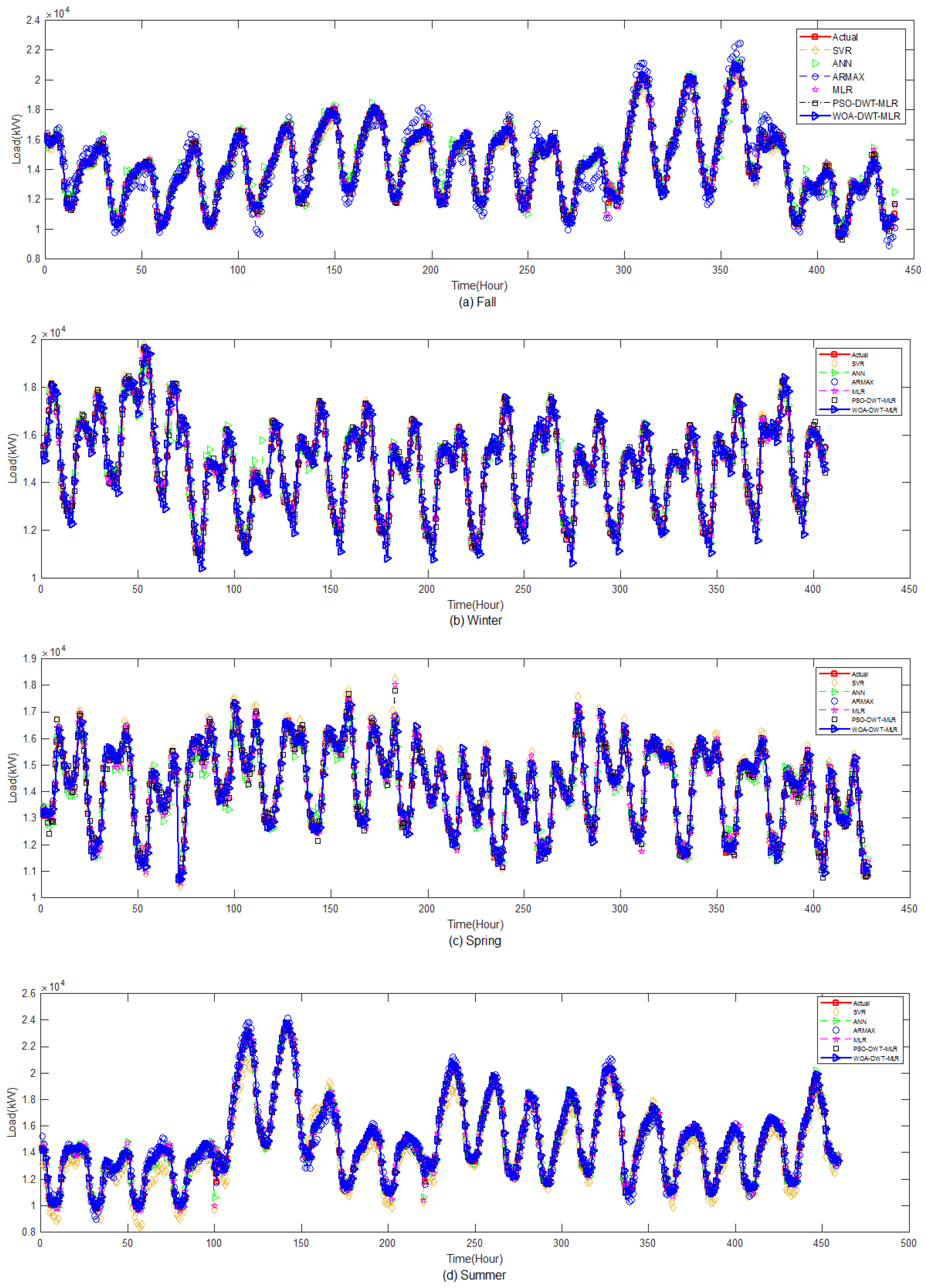
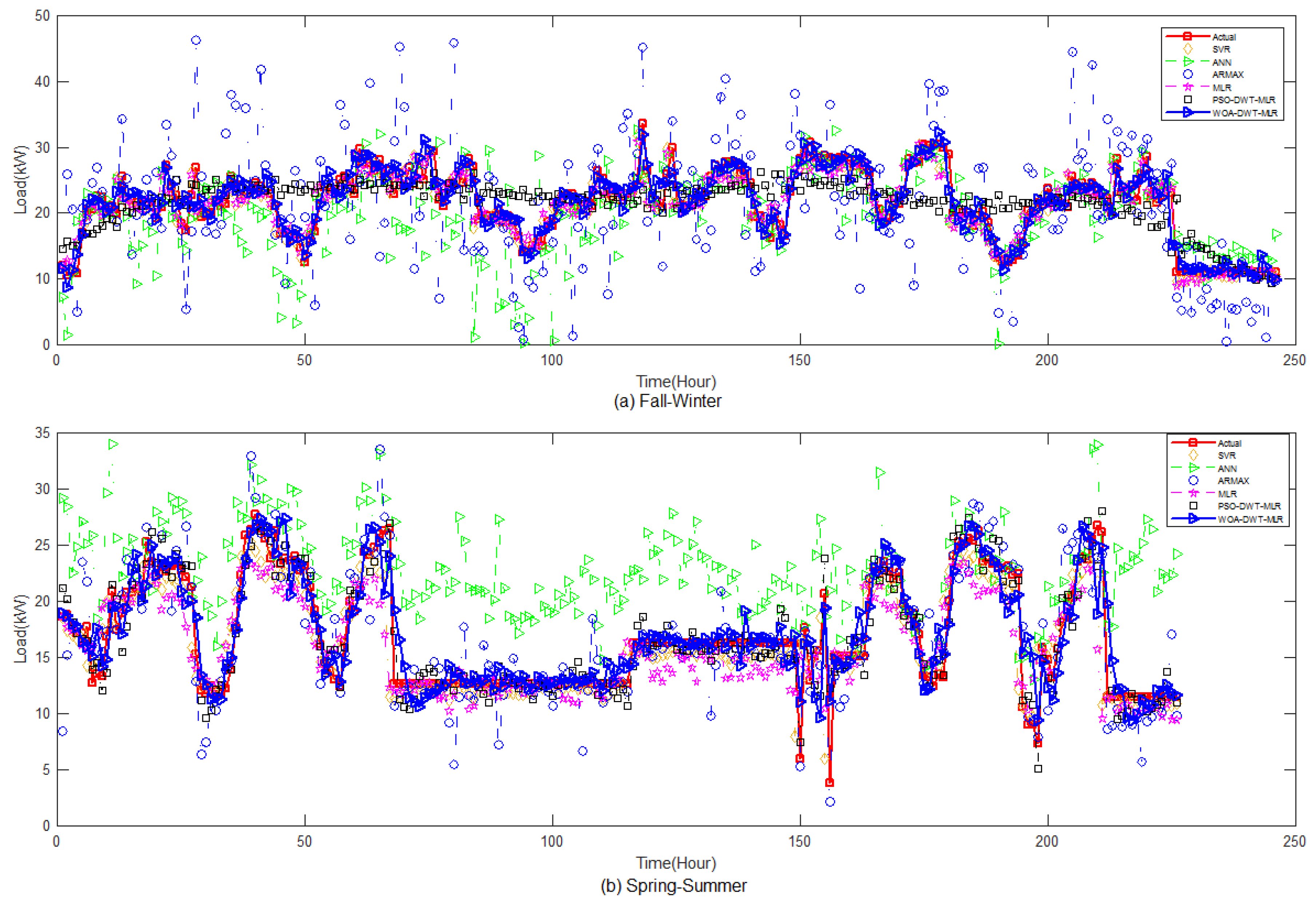
To get deeper observation of the prediction results of the proposed method, we extended the prediction period into several days for each season in the ISO-NE and Shalun data set, as depicted in Figure 11 and Figure 12, respectively. It is noted that, due to some missing data, the pattern of some hours of a day is neglected to avoid greater error in prediction evaluation. From these figures, we can infer that both the system and end-user data set are non-stationary with weekly seasonality and seasonal trends, even though we have treated the data based on its season. Especially in the Shalun data set, as seen in Figure 12, the seasonal trend is distinct because of the combination of seasons in Fall-Winter and Spring Summer groups, due to lack of data.

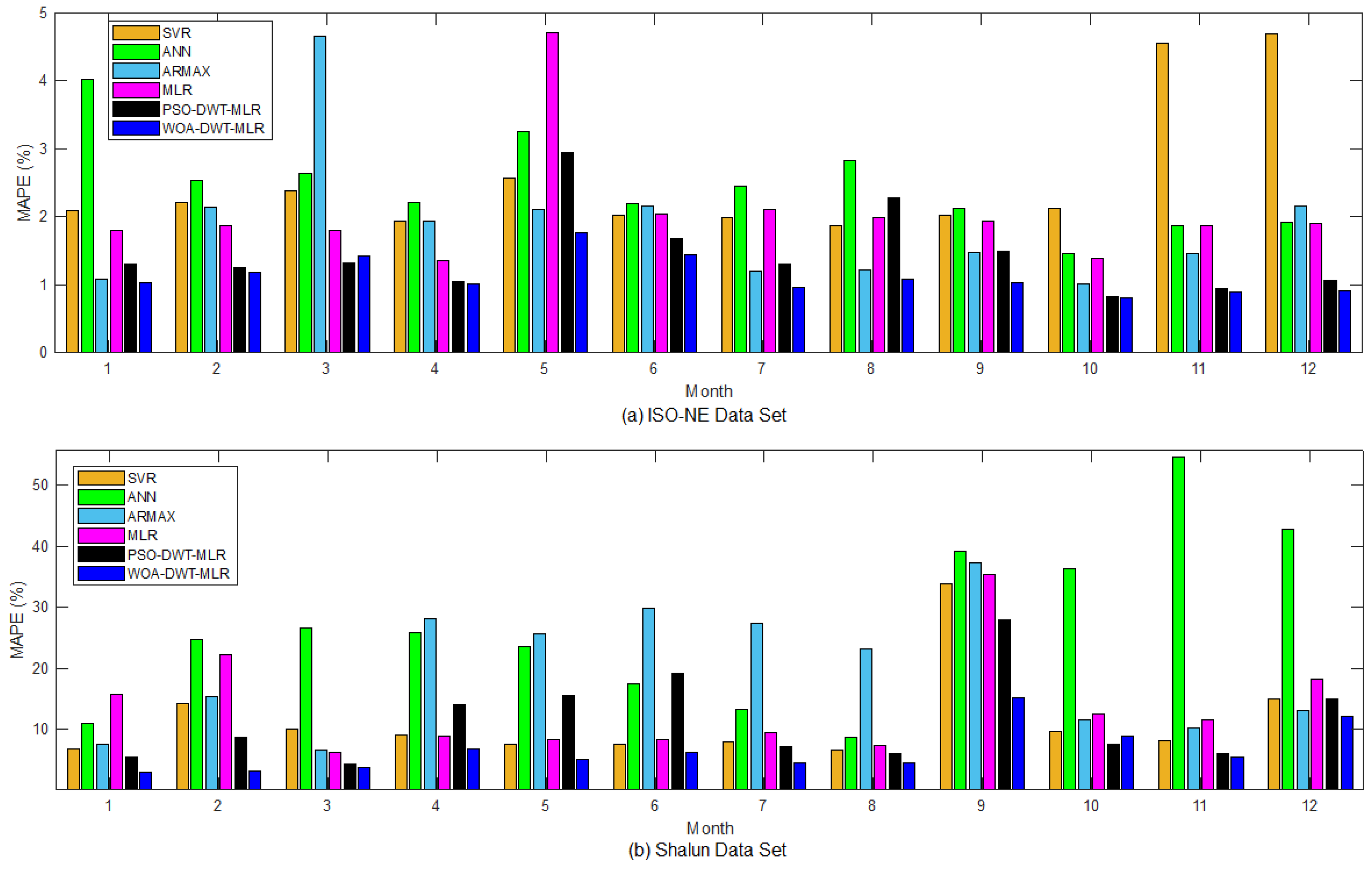
To avoid subjective judgement based on visual observation of the prediction pattern results, the annual averages of MAPE for both the ISO-NE and Shalun data sets are plotted monthly in Figure 13a,b, respectively. Axis-y represents the average MAPE of the month, while axis-x represents month with month-1, month-2, …, and month-12 being January, February, …, and December. For the ISO-NE data set, as shown in Figure 13a, we can observe that prediction techniques without discrete wavelet transform do not have better accuracy due to its inability to extract nonstationary part of the load pattern. Besides, though ARMAX can produce a mostly better performance in January, July, August, September, and October, the prediction performance is gets worse in the other months, showing an unsteady prediction performance of ARMAX.

Different from the former prediction techniques, the prediction result of PSO-DWT-MLR and WOA-DWT-MLR are more stable in magnitude of 1% to 3% MAPE and 1% to 2% of MAPE, respectively. For the PSO-DWT-MLR, the MAPE in May and August is worse than traditional MLR because of the PSO trapped at the local minima. Thus, though DWT is already used, the combination of approximation and detailed component cannot effectively produce accurate prediction. For the proposed WOA-DWT-MLR, the MAPE is higher in May for about 1.77% but quite stable at 0.98% of MAPE for the remaining months. As shown in Figure 13b for the Shalun data set, the performance of WOA-DWT-MLR is better than other comparison methods. Though, in September, the MAPE is higher, up to 15.21%, in comparison, the comparison method has 33.82%, 39.29%, 37.27%, 35.45%, and 28.01% for SVR, ANN, ARMAX, MLR, and PSO-DWT-MLR, respectively. The main cause of the higher errors in September comes from the data scarcity due to too many bad data.

For the end-user data set, the prediction accuracy of all the methods for comparison is worse than the ISO-NE data set because of its irregular power consumptions. Though relevant weather information has been selected, the other exogenous factors, like user behavior, still highly affect the randomness in the load consumption pattern. Further disturbing the load pattern for the tuning stage, the irregularity is also worsened by the outlier data due to out of order of the communication system for collecting the load data. Therefore, in further research, a more reliable data preconditioning scheme is needed to support the prediction modeling.

Related to the length of available data, the proposed method has strong consistency in accuracy, as proved by the MAPE. The accuracy is not bounced away when facing a lack of data, such as that happening in the Summer and Fall model, when the other methods lose their accuracy. It reveals that the proposed method can handle the highly nonlinear end-user data set, while the other methods fail to maintain their accuracy.

For the computation time, the proposed method constructs the final prediction model by storing the best information of MLR coefficients, type of DWT, and level of wavelet decomposition in each iteration. Without the WOA-DWT, MLR needs less than 1 min to build a load forecasting model, while ANN and ARMAX require more computation time. After the WOA-DWT strategy applied in MLR by the proposed method, the computation time increases to several minutes and up to ten minutes. Once the testing stage begins, the algorithm needs to manage the process of wavelet decomposition and requires more time than the other methods to produce prediction but fits the application requirement.

6. Conclusions

This paper has proposed an open-ended STLF algorithm that works in both system- and end-user data sets. The algorithm uses WOA to find the optimal level of decomposition, type of wavelet, and reconstruction of detail and approximation components in an MLR-based prediction model. WOA is proved to be more efficient in finding global optimum in wavelet decomposition. From results of validation and testing stages, the proposed WOA-DWT-MLR method has been proved to predict with better accuracy as compared to the MLR, ANN, ARMAX, SVR, and PSO-DWT-MLR approaches. Especially for the end-user data set, the proposed method outperforms the compared methods significantly in the prediction consistency. However, the computation time can be further addressed due to the usage of WOA-DWT in the reconstruction process at the training stage, though it is still manageable to be performed for day-ahead load forecasting. Nevertheless, the proposed method has shown promising results for further use in an offline system, such as the planning of demand response or in an energy management system. Furthermore, the proposed method can be extended as the base prediction model for probabilistic load forecasting, due to its ability in providing consistent and accurate prediction results.