Analysis of the Nexus of CO₂ Emissions, Economic Growth, Land under Cereal Crops and Agriculture Value-Added in Pakistan Using an ARDL Approach

Abstract

The present study attempts to explore the correlation between carbon dioxide emissions (CO₂ e), gross domestic product (GDP), land under cereal crops (LCC) and agriculture value-added (AVA) in Pakistan. The study exploits time-series data from 1961 to 2014 and further applies descriptive statistical analysis, unit root test, Johansen co-integration test, autoregressive distributed lag (ARDL) model and pairwise Granger causality test. The study employes augmented Dickey–Fuller (ADF) and Phillips–Perron (PP) tests to check the stationarity of the variables. The results of the analysis reveal that there is both short- and long-run association between agricultural production, economic growth and carbon dioxide emissions in the country. The long-run results estimate that there is a positive and insignificant association between carbon dioxide emissions, land under cereal crops, and agriculture value-added. The results of the short-run analysis point out that there is a negative and statistically insignificant association between carbon dioxide emissions and gross domestic product. It is very important for the Government of Pakistan’s policymakers to build up agricultural policies, strategies and planning in order to reduce carbon dioxide emissions. Consequently, the country should promote environmentally friendly agricultural practices in order to strengthen its efforts to achieve sustainable agriculture.

1. Introduction

The changes in climate affect the productivity of the agriculture sector through a variation in global temperatures, the variability of precipitation and other related factors. It is estimated that about 15%–30% of the output of agriculture would be affected negatively by 2080–2100 [1]. A further decline in crop yield may occur in Africa, Latin America and Asia because adaptive measures are overlooked. The Fourth Assessment Report of the Intergovernmental Panel on Climate Change stated that it would cost about 5%–10% of GDP for Africa to take adaptation measures to combat climate change [2]. Moreover, they predicted that about a 50% drop in agricultural crops would be observed by 2020 and the crop revenue may further decrease even up to 90% by 2100. The variation in the pattern of rainfall has also affected more than one billion people in South Asia [3]. Researchers including [4,5,6,7,8,9,10,11,12,13,14,15] and many others have shown that climate change poses threats to agriculture, food and water supplies, especially in the developing economies. Most of the models indicate that climate variation would adversely affect the yield of wheat in South Asia. The Intergovernmental Panel on Climate Change (IPCC) 4th Assessment Report put forth that in South Asia the crop yield would reduce proportionately from 1820 m³ to 1140 m³ from 2001 to 2050.

The increasing population of Pakistan and non-assurance of food security for its society is a challenge, since the residents are expected to double by 2050 [16]. Climate change and adaptation strategies are increasingly becoming the main focus of scientific research these days, for instance, the effect on the production of crops such as wheat, rice and maize [17]. The vulnerability index of the fluctuation of climate in Pakistan is remarkably rising in comparison to numerous countries around the globe, due to variable climatic conditions. Of late, Pakistan has been confronted with a lot of climatic variations, for instance; a rise in temperature, changes in the pattern of precipitation, floods, earthquakes and weather shifts. The development of the agriculture sector in developing countries is hampered by increasing climatic risk and projected changes in climate over the 21^st century [18]. Pakistan is affected the most by climate change owing to inadequate and substandard infrastructure and limited adaptive capacity [19]. It is projected that by 2050, there would be a 2%–3% rise in temperature causing a significant variation in the pattern of rainfall [20]. The country is ranked 8 among the most negatively affected countries by adverse weather conditions and climate change over the period 1995–2014 as reported by the Global Climate Risk Index (GCRI) [21]. The productivity of the main crops including wheat, rice, cotton and sugarcane and rural livelihoods has been affected significantly due to climate variability and extreme events over the last two decades [22]. The vulnerability of rural livelihood to climate change can be seen from the historic floods during 2010–2014 and severe droughts from 1999 to 2003 [22]. Greenhouse gas emissions may cause an unproductive effect on the environment up to a great extent and this issue becomes substantially critical for all countries in the world. Recently, many researchers have been paying attention to the carbon dioxide emissions as one of the essential causes of global warming [23,24,25,26]. There has been an unprecedented increase in population, agricultural production, energy demand and economic growth to achieve food security, and carbon dioxide emissions have also increased over the decades [27,28,29,30].

In this study, we conducted an in-depth investigation of the entire country (Pakistan) which explores the variety of responses of the carbon dioxide emissions (CO₂ e), gross domestic product (GDP), land under cereal crops (LCC) and agriculture value-added (AVA) based on historical data during 1961 to 2014. The autoregressive distributed lag (ARDL) model is employed simultaneously to observe the effect of the CO₂ e, GDP, LCC and AVA in order to identify a certain correlation between them. This enabled us to determine the long-run relationships among several variables [31]. Johansen and Juseliu’s estimation to carefully investigate this subject in-depth. In addition, we also conducted generalized impulse response functions and variance decomposition methods to find out the effects of shocks on the adjustment path of the variables.

The rest of the study is structured as follows: the second section entails a brief part of the literature review. The third section is about the research methodology refers to the processing for the data collection. The fourth section is the results and discussion part and the final section is the conclusion and policy recommendations of the study in hand.

2. Literature Review

A wide range of literature is accessible on determining the factor of economic growth, agricultural production and the emissions of carbon dioxide. The long-run equilibrium relationship between carbon dioxide emissions, income growth, energy consumption and agriculture for Pakistan from 1971 to 2014 have been verified and tested. The results confirmed that there were bidirectional causalities between GDP, agriculture, energy use and CO₂ emissions. They also found that AVA had a positive inelastic effect on CO₂ emissions and that GDP had a positive elastic impact on CO₂ emissions [32]. The previous study investigated the impact of AVA and per capita renewable energy consumption on carbon dioxide emissions in Asian countries. They found that agricultural and renewable energy had negative impacts on CO₂ emissions [33]. Evidence from the study revealed long-run equilibrium association flowing from consumption of electricity industrialization, gross domestic product and carbon dioxide emissions [34]. The study employed the vector error correction model (VECM) and ordinary least squares (OLS) regression revealed the effect of population progression, energy intensity and GDP on carbon dioxide emissions in Ghana. The study provided evidence of the existence of long-run equilibrium association flowing from population growth, energy intensity and gross domestic product to carbon dioxide emissions. The study also revealed that there was a bi-directional causality among energy consumption and carbon dioxide emissions [35]. Another study in Ghana investigated the association between population growth, use of energy, gross domestic product and carbon dioxide emissions by using both ARDL regression analysis and VECM. The study found that there will be fluctuation in carbon dioxide emissions due to the use of energy in the future. Evidence from the study showed a unidirectional causality running from carbon dioxide emissions to the use of energy and population [29]. Another study in China employed the ARDL model, the Granger causality test based on VECM, and impulse response and variance decomposition to test the relationship between CO₂ emissions, energy consumption and economic growth in the agricultural sector. The estimated results illustrated that there is bidirectional causality between agricultural carbon emissions and agricultural economic growth in both the short run and long run and there exist unidirectional causality from agricultural energy consumption to agricultural carbon emissions and agricultural economic growth [36]. The empirical results derived from the study confirmed the validty of the environmental Kuznets curve (EKC) hypothesis for three countries namely France, Portugal and Spain during the period under the study in the long-run as well as in short-run with exception the case of Portugal [37].

It is evident that a rise in temperature can have a devastating effect on the productivity of the agriculture sector, food security and farmers’ incomes. This phenomenon varies in tropical and temperate zones. In the middle- and the high-latitude zones, the output of crops is anticipated to increase and spread northwards and vice versa for several other countries in tropical regions [38]. It has been found that high latitudes can cause an expansion in the production by nearly 10% due to a 2 °C rise in temperature, whereas it reduced production just by the same percent in the low latitude. Considering the inevitable effect of contemporary technology, it is projected that an increase in temperature would increase the productivity of yield by 37% and 101% by 2050s for the Russian Federation [39].

As compared to other developing countries, the effects of escalating temperature on agriculture are harsher in Sub-Saharan Africa [40]. It has been observed that some important climatic conditions such as temperatures and rainfall had persisted at their pre-1960 status, then the gap of agricultural production between different developing countries and Sub- Saharan Africa at the end of the 20th century would have remained only 32% of the existing shortfall. A study for the period of 1980–2005 in Nigeria indicated that temperature exerts a negative effect while rainfall has a positive effect on agricultural production [41].

Another study developed a two-chain logarithmic mean divisia index (LMDI) decomposition method and derived the results that technology, distribution and population effects could not suppress China’s agricultural carbon dioxide emissions simultaneously in most years [42]. Developed countries have the ability to maintain a minimum level of technology for the improvement of living standards and increasing agricultural productivity [43]. Generally, developed countries are capable of counterbalancing the negative consequences of climate change. Developed states usually have a low level of susceptibility but a high level of adaptive ability, which itself has a role of technological expertise, dissemination and supply of assets, and human social and political capital [44]. The developed world has very standard levels of water filtration and sanitation; on the other hand, developing countries have insecure and unreliable water supplies and often the sanitation system is non-satisfactory and below the margin. The concept of crop insurance is utterly missing in developing countries to protect their farmers from the negative consequences of climate change which may destroy their livelihoods.

Since the last decade, the country’s (Pakistan) per capita GDP has observed a diverse or unlike trend and lack of equilibrium. During the period from 2005 to 2014 the per capita GDP increased from 974.5$ to 1111.2$ respectively. In 2011, the government gave great importance ton upgrading the country’s economy and can be witnessed that per capita GDP has consistently increased during the period 2011 to 2014. During the period of 2011 to 2014, even though there were several types of socio-economic challenges such as energy crises, a war against terrorism and poverty, still there was a rise of 64.71$ in per capita GDP (Pakistan Economic Survey 2017). In consequence, it is evident that the Government of Pakistan has taken actions to raise economic growth and enriched living conditions.

3. Methodology and Data Collection

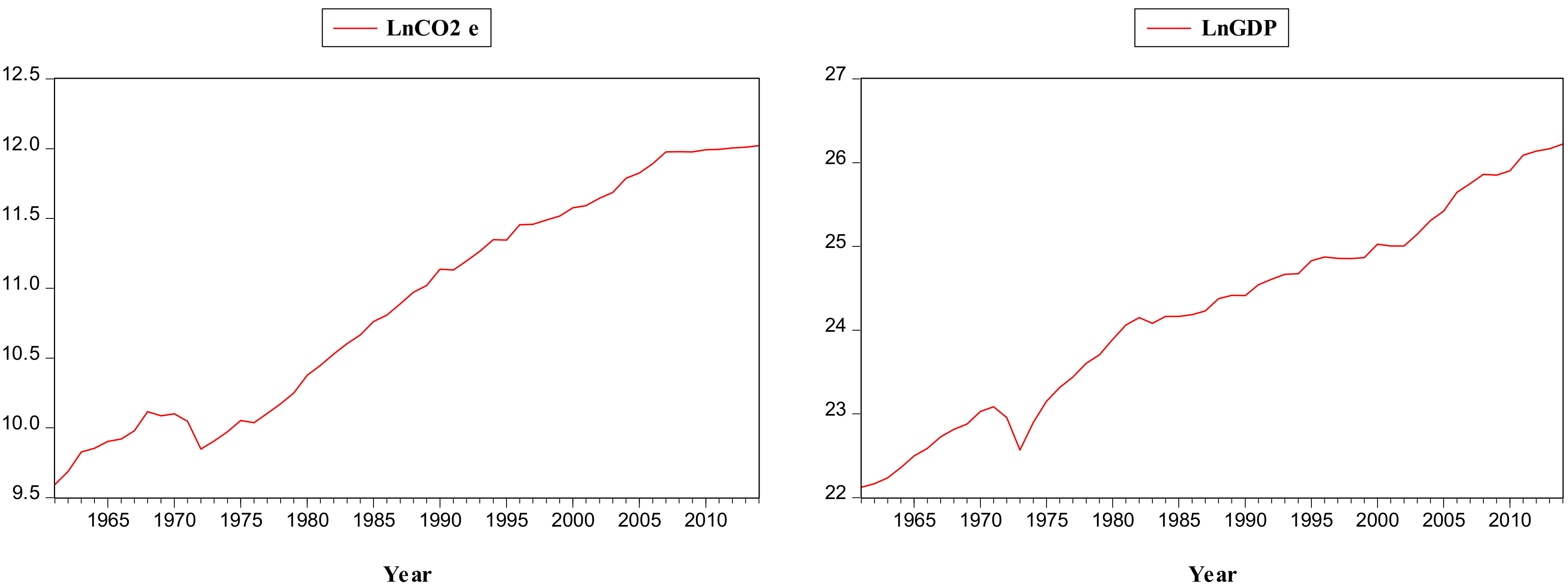
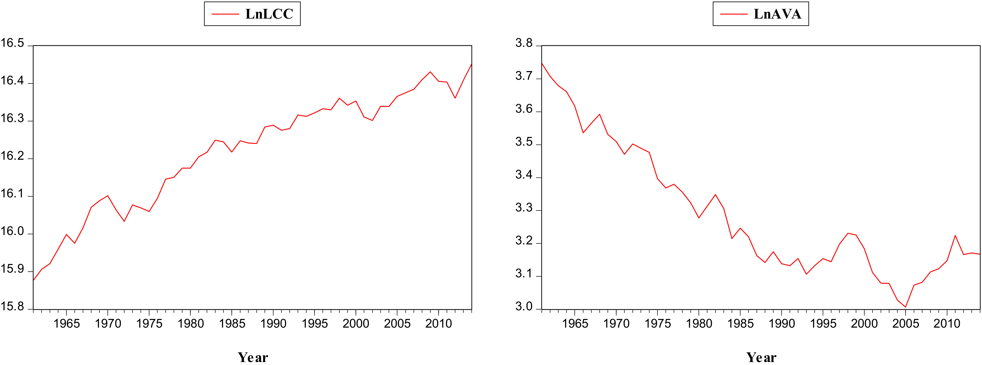
3.1. Data Sources and Description

The fundamental purpose of the aforementioned study is to find out the relationship between CO₂ e, GDP, LCC and AVA in Pakistan. The study adopted the time series data spanning from 1961 to 2014 using the ARDL method to test the relationship between study variables. To fulfill the study objectives, the data sets of the selected variable in the study were procured from the Food and Agriculture Organization Corporate Statistical Database FAOSTATS (www.fao.org) and World Development Indicators (http://data.worldbank.org).

Four variables were considered throughout the analysis where carbon dioxide emissions CO₂ e (kt) was taken as a dependent variable and explanatory variables include GDP (current US$), LCC (hectares) and AVA (percentage of GDP). This study employed the actual CO₂ emissions instead of potential CO₂ (i.e., CO₂ eq.). Previous studies [29,45,46] put into practice the actual CO₂ emissions which show that the use of actual CO₂ emissions improves the efficiency of the model.

Table 1. Detail of variables.

Variable Name	Abbreviation	Unit of Measurement	Source
Carbon dioxide emission	CO2 e	Kilotons (kt)	FAOSTAT (2018)
Gross domestic product	GDP	Current US $	WDI (2018)
Land under cereal crop	LCC	Hectares	WDI (2018)
Agriculture value added	AVA	Percentage of GDP	WDI (2018)

shows the source of data and variable description. The trend analysis of the study variables are given Figure 1.

3.2. Econometric Model

The current study entails the co-integration and autoregressive distributed lag model to find out the association between carbon dioxide emissions, gross domestic product, land under cereal crop and agriculture value-added in Pakistan. The following steps show our study analysis. In the first step, we have to find out the stationarity in the time series data. For this objective, we conducted the augmented Dickey-Fuller (ADF) test [47] and Phillips and Perron (PP) unit root tests [48]. The step second was to find out the optimal lag length of the study variables. To determine the lag lengths we used the Akaike information criterion (AIC) [49] or Schwarz information criterion (SIC) [50]. In the third step, we estimated the Johansen co-integration test to seek the long-run relationship between the study variables. Were there a co-integration, then we moved to the next step. In the last step, were a co-integration to exist then we estimated an ARDL model. Furthermore, we also estimated the pairwise Granger causality test to establish causal links between variables. The econometric model used in this study is given as:

$$C{O}_{2 et}=f\left(GD{P}_t,LC{C}_t,AV{A}_t\right)$$

(1)

where in the above equation (1), CO₂ e is the carbon dioxide emissions, GDP is the gross domestic product, LCC is the land under cereal crop, AVA is the agriculture value-added and t is the time period. We then applied the Cobb Douglas production function in its stochastic form as:

$$C{O}_{2 et}={\alpha }_0{\alpha }_{1}GD{P}_t,{\alpha }_{2}LC{C}_t,{\alpha }_{3}AV{A}_t$$

(2)

Then we employed the log-linear model, for this purpose, we log-transform the above model to get the linear regression model which is given as:

$$lo{g}_e(C{O}_{2 et})={\alpha }_0+\sum lo{g}_e\left({\alpha }_{1}GD{P}_t,{\alpha }_{2}LC{C}_t,{\alpha }_{3}AV{A}_t\right)$$

(3)

Then we transformed the variable’s value into their natural logarithm form to find out the long-run association between the study variables. This transformation of the data into their natural logarithm is to ensure the results were efficient, reliable and consistent. Equation (4) shows the logarithm form for the study variables.

$$lnC{O}_{2 et}={\alpha }_0+{\alpha }_{1}lnGD{P}_t+{\alpha }_{2}lnLC{C}_t+{\alpha }_{3}lnAV{A}_t + {\epsilon }_t$$

(4)

where lnCO_{2 et} lnGDP_t, lnLCC_t and lnAVA_t expressed the natural logarithm of carbon dioxide emissions, gross domestic product, crop production index, land under cereal crop and agriculture value-added, respectively. In the above equation (4), t =1,…….N represents the time period and ${\epsilon }_t$ is the error term. The parameters ${\alpha }_0,{\alpha }_1, {\alpha }_2,and {\alpha }_3$ measure the long-run elasticity of carbon dioxide emissions with respect to the real GDP, land under cereal crop and agriculture value-added respectively.

4. Results and Discussions

4.1. Descriptive Analysis and Correlation Matrix

The descriptive analysis shows mean, coefficient of variation, skewness, kurtosis and normality of distribution over the study variables.

Table 2. Descriptive statistics and correlation matrix of all the variables.

Variables	LnCO2 e	LnGDP	LnLCC	LnAVA
Mean	10.88533	24.21358	16.22058	3.290421
Median	10.92998	24.30179	16.24839	3.222102
Maximum	12.02154	26.22191	16.45170	3.746831
EMinimum	9.592673	22.12312	15.87711	3.006656
Std. Dev.	0.801811	1.193248	0.152553	0.196416
Skewness	0.002686	−0.087221	−0.548516	0.734181
Kurtosis	1.510778	1.953711	2.226820	2.385217
Jarque-Bera	4.990073	2.531587	4.052896	5.701605
Probability	0.082493	0.282015	0.131803	0.057798
Correlation
LnCO2 e	1.000000
LnGDP	0.978197	1.000000
LnLCC	0.956098	0.973567	1.000000
LnAVA	−0.884455	−0.897413	−0.930411	1.000000

provides the descriptive analysis and the kurtosis results display that all the variables exhibit platykurtic distribution. The results of the skewness indicate that both carbon dioxide emissions and agriculture value-added have long right-tail distribution while the remaining variables indicate long left-tail distribution. The outcome from the Jarque–Bera test shows that we accept the null hypothesis of normal distribution at the 5% level of significance for all variables except agriculture value-added. The mean results show that the gross domestic product generate a high value of 24.21. The standard deviation analysis show that the gross domestic product is also the most explosive variable with the highest deviation of 1.19 followed by carbon dioxide emissions.

4.2. Lag Selection for Vector Error Correction Model

After the unit root test, in the next step we need to find out the optimum lag length for co-integration analysis by using the AIC criteria [49] or SIC [50] criteria. The AIC results in

Table 3. Selection of lag length.

Lag	LogL	LR	FPE	AIC	SC	HQ
0	112.9309	NA	1.51e–07	−4.357238	−4.204276	−4.298989
1	346.9699	421.2700	2.46e–11	−13.07879	−12.31398*	−12.78755*
2	366.4259	31.90793*	2.17e–11*	−13.21704*	−11.84038	−12.69280
3	380.8168	21.29858	2.39e–11	−13.15267	−11.16417	−12.39544
4	395.6585	19.59104	2.67e–11	−13.10634	−10.50599	−12.11611

* indicates lag order selected by the criterion; e: stands for exponential constant; LR: sequential modified LR test statistic (each test at 5% level); FPE: Final prediction error; AIC: Akaike information criterion; SC: Schwarz information criterion; HQ: Hannan-Quinn information criterion.

indicate that the most suitable lag value is lag 2 for the model.

It is important to find out how many lags to be used in ARDL model. Therefore, to figure out the optimal number of lags for the model, the unrestricted vector autoregression (VAR) lag selection criteria is tested. Table 3 formulates the lag selection criteria for the model but the most commonly employed criteria are AIC and SIC. The previous study used AIC for a small sample size [51].

4.3. Unit Root Test

Before estimating the co-integration analysis, it is important to determine where the study variables are stationary at first difference i.e., I(1). The stationarity of the variables is tested using the ADF test [47] and PP test [48] in order to have a robust result and avoid spurious regression results.

Table 4. Unit root test (Augmented Dickey–Fuller).

Variables	Akaike Info Criterion				Philips–Perron
	LEVEL		1ST DIFFERENCE		LEVEL		1ST DIFFERENCE
	Intercept	Trend and Intercept	Intercept	Trend and Intercept	Intercept	Trend and Intercept	Intercept	Trend and Intercept
LnCO2 e	−0.63771 0.8528	−2.107644 0.5292	−5.915923 0.0000	−2.908476 0.1689	−0.809440 0.8082	−1.554595 0.7974	−5.928838 0.0000	−5.897317 0.0001
LnGDP	−0.512237 0.8803	−3.102790 0.1165	−6.128411 0.0000	−6.074545 0.0000	−0.501008 0.8825	−2.682416 0.2478	−6.117041 0.0000	−6.043380 0.0000
LnLCC	−1.845078 0.3552	−3.097552 0.1175	−7.310103 0.0000	−5.882637 0.0001	−2.177064 0.2168	−3.058810 0.1268	−7.399540 0.0000	−7.703130 0.0000
LnAVA	−2.617304 0.0959	−1.487037 0.8218	−6.708506 0.0000	−4.529780 0.0039	−2.720270 0.0773	−1.506937 0.8148	−6.708506 0.0000	−7.242419 0.0000
Conclusion	Non-stationary		Stationary		Non-stationary		Stationary

shows the unit root test results. Our findings in Table 4 indicate that all the study variables are non-stationary at a level. However, the variables became stationary at their first difference and rejected the null hypothesis that unit root exists at first difference. The results show that all the study variables are stationary at first difference which means that variables are integrated at I(1). Since the variables entailed in the study are I(1), so this indicates the spurious regression problem occurs here. Hence it is important to find out the co-integration test among the time series variables.

4.4. Johansen Co-Integration Test

A summary of the Johansen co-integration [52] test is presented in

Table 5. Results of Johansen co-integration test.

Hypothesized No. of CE(s)	Rank Test (Trace)				Rank Test (Maximum Eigenvalue)
	Eigenvalue	Trace Statistic	0.05 Critical Value	Prob.	Max-Eigen Statistic	0.05 Critical Value	Prob.
None	0.423351	52.89693	47.85613	0.0156	28.07661	27.58434	0.0432
At most 1	0.300607	24.82032	29.79707	0.1679	18.23469	21.13162	0.1213
At most 2	0.121100	6.585634	15.49471	0.6263	6.583293	14.26460	0.5395
At most 3	0.0000459	0.002341	3.841466	0.9593	0.002341	3.841466	0.9593

. The purpose of the Johansen co-integration test is to find out the long-run relationship between the study variables in the model. Maximum eigenvalue and trace statistic tests [53] were conducted to determine the co-integration among the study variables. The results of the maximum eigenvalue and trace statistic showed 4 co-integrating equations at the 5 percent level. Here, the results of co-integration would determine whether we have to apply a VAR model or VECM model.

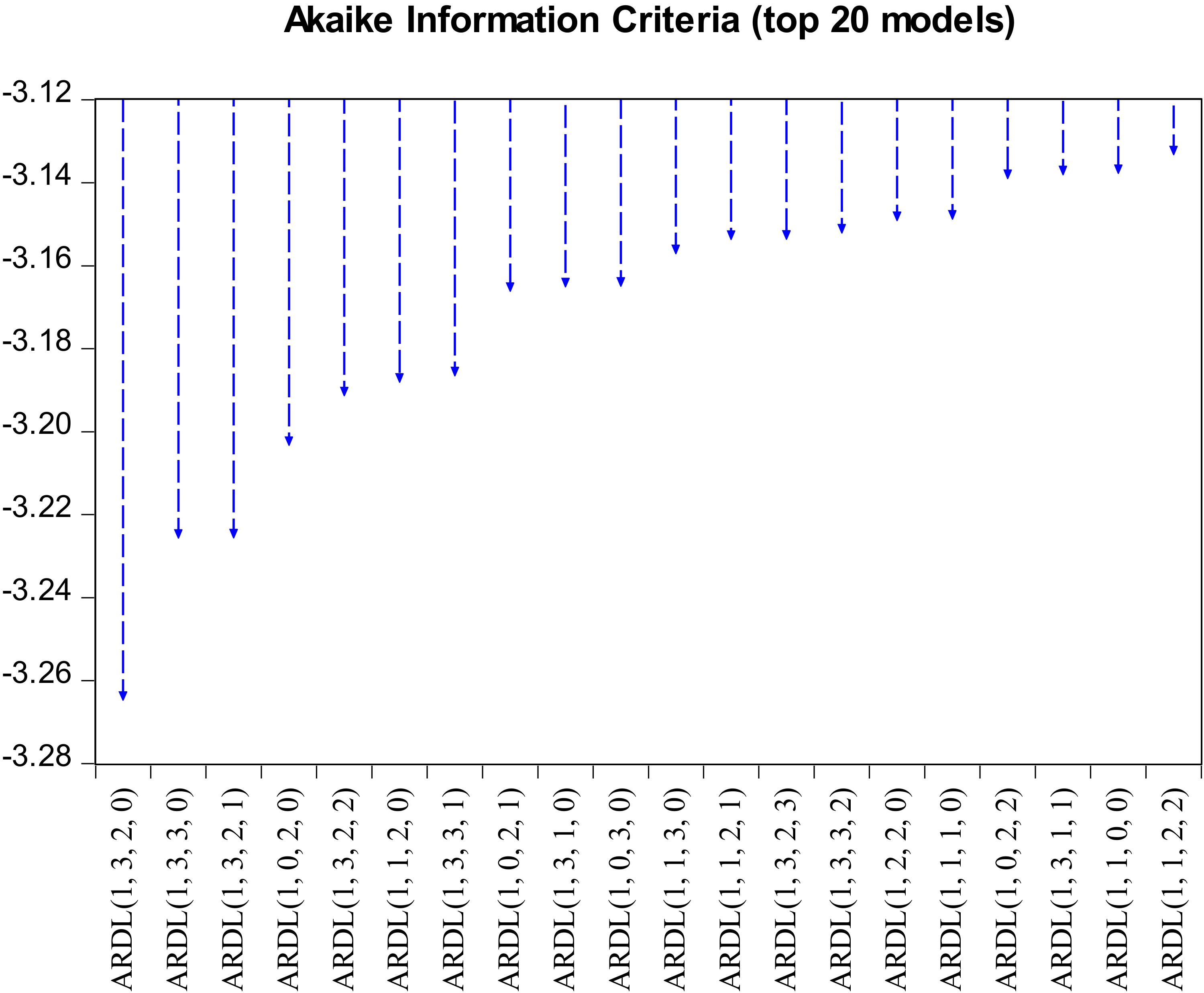
4.5. Autoregressive Distributed Lag (ARDL) Bound Testing of Co-Integration

The current study uses an ARDL bound testing approach suggested by [54] to find out both short-run and long-run association of the CO₂ e, GDP, LCC and AVA. The ARDL bound testing method is appropriate for those models in which there is a mixture of I(0) and I(1) variables. Another characteristic of this model is that it is appropriate for a small sample size as our sample size is only 52 [54].

After the estimation of unit root testing which shows that all variables are integrated at I(1), now we carried out the ARDL method of co-integration (bounds testing) to estimate the relationship between the selected variables in this study. The results of the ARDL bound testing are reported in

Table 6. ARDL bound testing.

Test Statistic	Value	k
F-statistic	5.805114	3
Critical Value Bounds
Significance	I(0) Bound	I(1) Bound
10%	2.37	3.2
5%	2.79	3.67
2.5%	3.15	4,08
1%	3.65	4.66

. The results indicate that the f-statistic value (5.805114) is greater than the 10% and 5% upper critical values of I(0) bound. The results of the bounds testing validate significant long-run relationships among variables and showing the rejection of null hypothesis of no co-integration association among LnCO₂ e, LnGDP, LnLCC and LnAVA.

Furthermore, the study estimates the AIC to prefer the optimal model by employing long-run and short-run association among variables. Employing the Akaike information criterion shows the top 20 possible ARDL models in Figure 2. Based on the model specification in equation (4), the short-run and long-run equilibrium relation LnCO₂ e, LnGDP, LnLCC and LnAVA is estimated using the ARDL regression analysis shown in equation (5) where

α₀ = 19.2356, α₁ = 0.3246, α₂ = −0.2867 and α₃ = −3.3902.

(5)

4.6. Short-Run and Long-Run Equation Models

Table 7. Short-run and long-run relationship estimates selected model for autoregressive distributed lag (ARDL) (1,3,2,0).

Short Run Coefficients
Variable	Coefficient	Std. Error	t-Statistic	Prob.
D(LnGDP)	0.033643	0.056658	0.593784	0.5559
D(LnGDP(−1))	0.014904	0.055969	0.266287	0.7914
D(LnGDP(−2))	−0.173688	0.058569	−2.965542	0.0050
D(LnLCC)	0.863260	0.241211	3.578864	0.0009
D(LnLCC(−1))	0.716364	0.243073	2.947112	0.0053
ECT(−1)	−0.077780	0.013781	−5.644230	0.0000
Long Run Coefficients
Variable	Coefficient	Std. Error	t-Statistic	Prob.
C	1.496155	4.774608	0.313357	0.7556
Ln CO2 e(−1)	−0.077780	0.038989	−1.994952	0.0527
LnGDP(−1)	0.025249	0.042403	0.595470	0.5548
LnLCC(−1)	−0.022297	0.326479	−0.068295	0.9459
LnAVA	−0.263688	0.097057	−2.716831	0.0096
D(LnGDP)	0.033643	0.063982	0.525816	0.6018
D(LnGDP(−1))	0.014904	0.065642	0.227049	0.8215
D(LnGDP(−2))	−0.173688	0.066271	−2.620874	0.0122
D(LnLCC)	0.863260	0.298943	2.887709	0.0062
D(LnLCC(−1))	0.716364	0.289813	2.471814	0.0177
EC = LnCO2 e − (0.3246(LnGDP) − 0.2867(LnLCC) − 3.3902(LnAVA) + 19.2356))

summarizes the results of short-run equation of the ARDL model. The results show that the speed of adjustment (error correction term ECT(−1)) value is –0.077780 which shows that there are a long run and short-run equilibrium relationships running from LnGDP, LnLCC and LnAVA to LnCO₂ e. The speed of adjustment is approximately 7.7 % in one period of long-run equilibrium.

Table 5 also shows the results of long-run equation results of the ARDL approach. The results of long-run equilibrium relationship show that a 1% increase in LnGDP will increase LnCO₂ e by 2%, a 1% increase in LnLCC will decrease LnCO₂ e by 0.02% and a 1% increase in LnAVA will decrease LnCO₂ e by 26% in long-run estimates.

The evidence of the following studies reveals that carbon dioxide emissions increase in the early phases of economic growth and then decline after a threshold point. The findings of these studies such as [10,55,56,57,58,59,60,61,62] examined the relationship between carbon dioxide emissions and GDP growth.

The findings of previous studies such as [63] for China, [59] for Tunisia, [64] for Iran, [65] for Pakistan, [66] for Malaysia, [57] for Turkey and [55] for India examined a unidirectional causality running from GDP income to carbon dioxide emissions without response which suggests that emission reduction plans will not restrain trade and industry growth and which seems to be a feasible policy instrument in the aforementioned studied countries to accomplish its long-run sustainable growth.

Furthermore, we applied generalized impulse response functions for the verification of the results. The generalized impulse response results show an in-depth understanding of shocks to gross domestic product, land under cereal crop, agriculture value-added affected carbon dioxide emissions. The results of generalized impulse responses for carbon dioxide emissions, gross domestic product, land under cereal crop and agriculture value-added are provided in Figure 3.

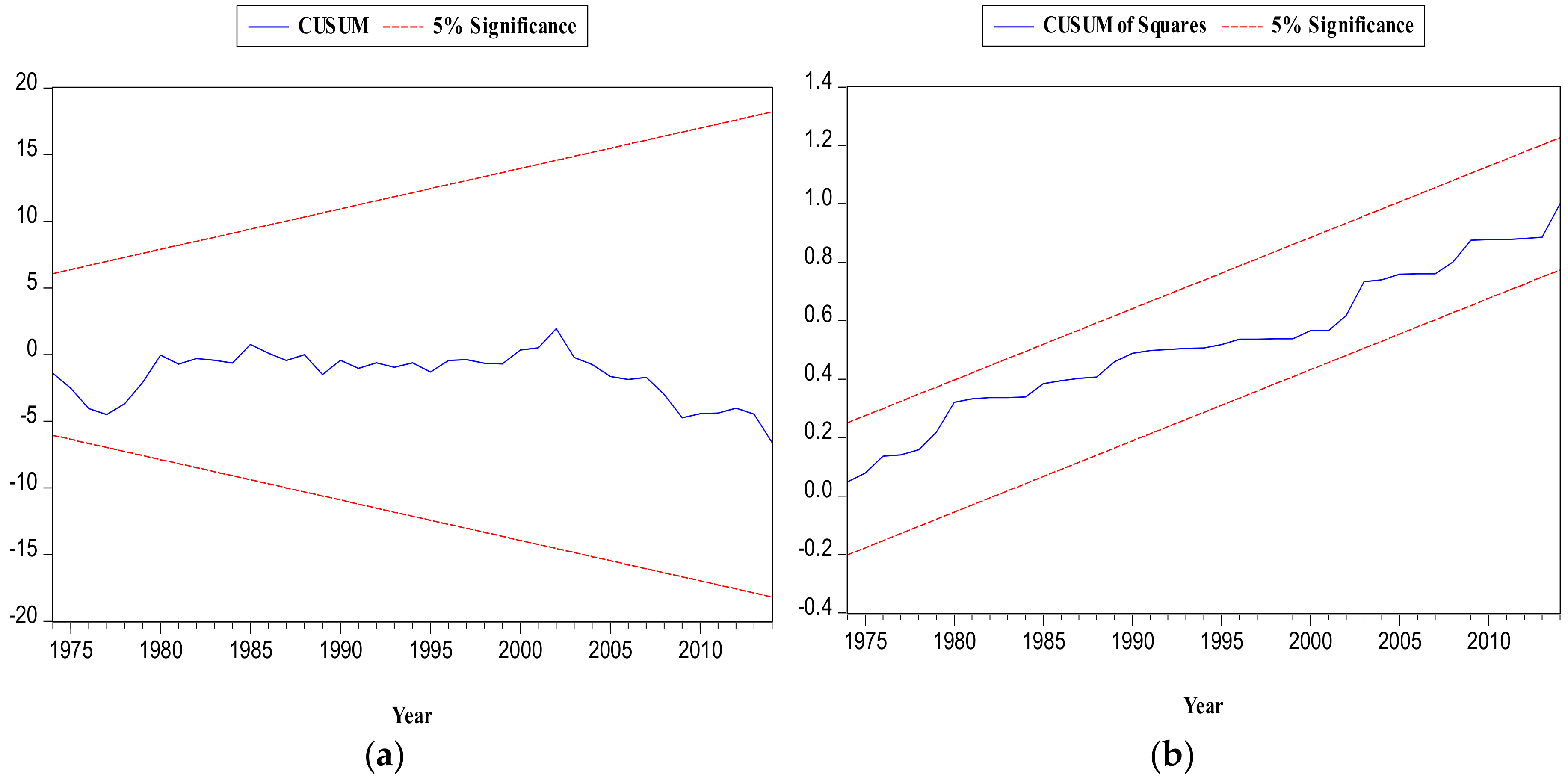
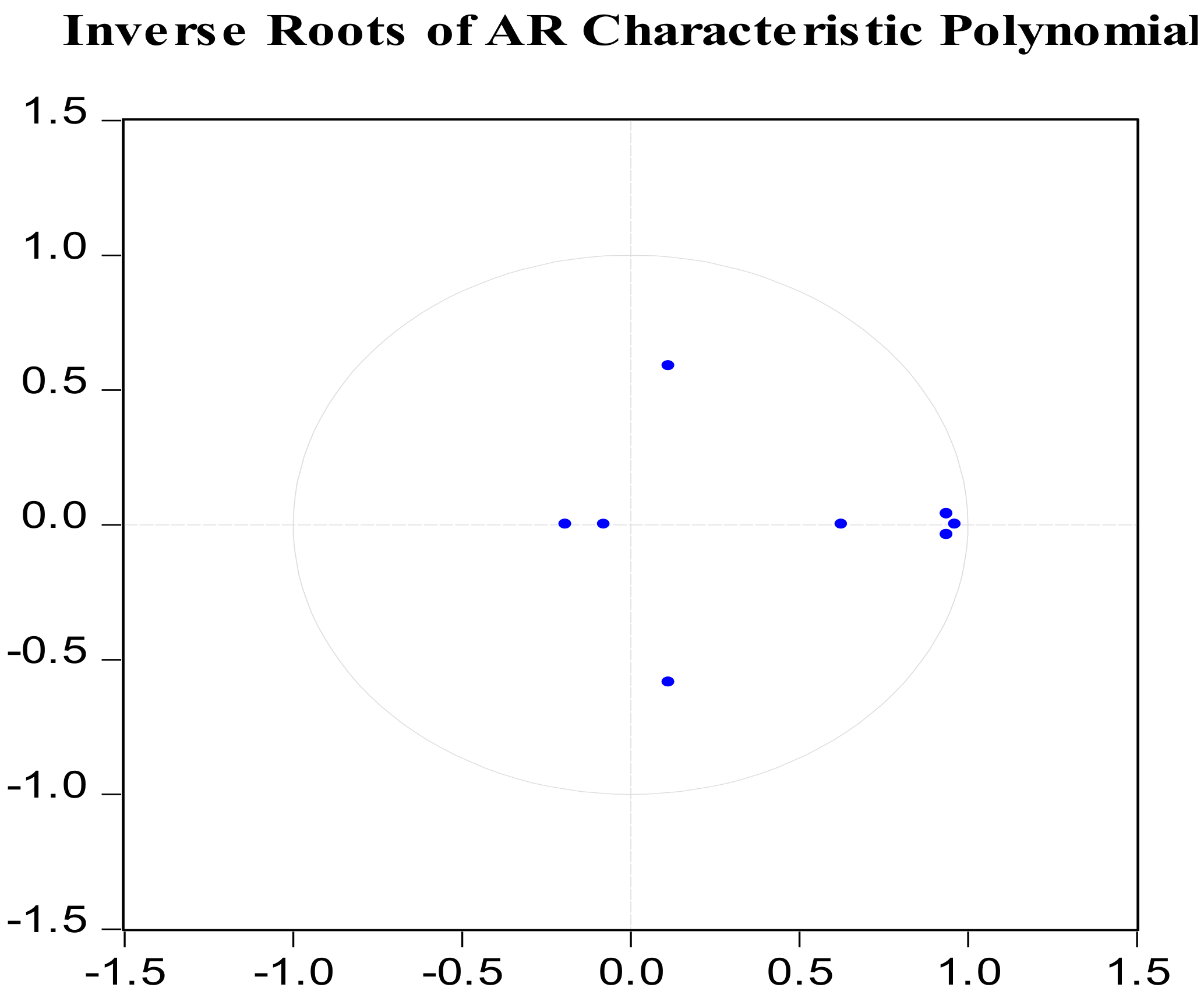
4.7. Diagnostic Test

As suggested by [67], both the cumulative sum of the recursive residuals (CUSUM) and the cumulative sum of the square of the recursive residuals (CUSUMsq) tests were implemented to run the ARDL model in a befitting manner. Figure 4 reveals that both the graphs of CUSUM and CUSUMsq tests lie between the critical bounds indicated with red colored lines at a 5% confidence interval. The blue color lines in the middle represent the measurements for the cumulative sum of the recursive residuals and the cumulative sum of the squares of the recursive residuals. Both CUSUM and CUSUMsq graphs show that the model of our study is well stable.

Several diagnostic tests were operated to check the good fit of the ARDL model.

Table 8. Diagnostic tests results.

Breusch-Godfrey Serial Correlation LM Test:
F-statistic	0.237056
Obs R-squared	0.936929
Prob. F(3,38)	0.8700
Prob. Chi-Square(3)	0.8165
Heteroskedasticity Test: Breusch–Pagan–Godfrey
F-statistic	1.190498
Obs R-squared	10.56646
Scaled explained SS	10.87174
Prob. F(9,41)	0.3268

shows that estimation is fine regarding the serial correlation Lagrange Multiplier (LM) test, where the F-statistics (0.237056) have insignificant probability. The heteroskedasticity test under Breusch–Pagan–Godfrey also signifies that there is no sign of serial correlation. The value of F-statistics (1.190498) shows an insignificant probability, which means there is no heteroskedasticity issue in the model estimation.

Furthermore, the inverse root of AR polynomial graph displaying the stability of the model where are blue dots is within the circle. Figure 5 shows the inverse root of AR polynomial estimation.

4.8. Pairwise Granger Causality Tests

The pairwise Granger causality test is estimated to find out the robustness of the model, which elaborates the directional linkages between the two variables at a time. The results of the pairwise Granger causality is exhibited in

Table 9. Pairwise Granger causality test.

Null Hypothesis:	Obs	F-Statistic	Prob.
LnGDP does not Granger Cause LnCO2 e	52	0.34510	0.7099
LnCO2 e does not Granger Cause LnGDP		8.51829	0.0007
LnLCC does not Granger Cause LnCO2 e	52	1.91090	0.1593
LnCO2 e does not Granger Cause LnLCC		1.81672	0.1738
LnAVA does not Granger Cause LnCO2 e	52	2.63228	0.0825
LnCO2 e does not Granger Cause LnAVA		0.42783	0.6544
LnLCC does not Granger Cause LnGDP	52	1.78823	0.1784
LnGDP does not Granger Cause LnLCC		6.22181	0.0040
LnAVA does not Granger Cause LnGDP	52	1.03562	0.3630
LnGDP does not Granger Cause LnAVA		0.13864	0.8709
LnAVA does not Granger Cause LnLCC	52	3.95660	0.0258
LnLCC does not Granger Cause LnAVA		1.43426	0.2485

. The estimations of the pairwise Granger causality shows unidirectional causality between LnGDP to LnCO₂ e, LnLCC to LnGDP and LnAVA to LnLCC.

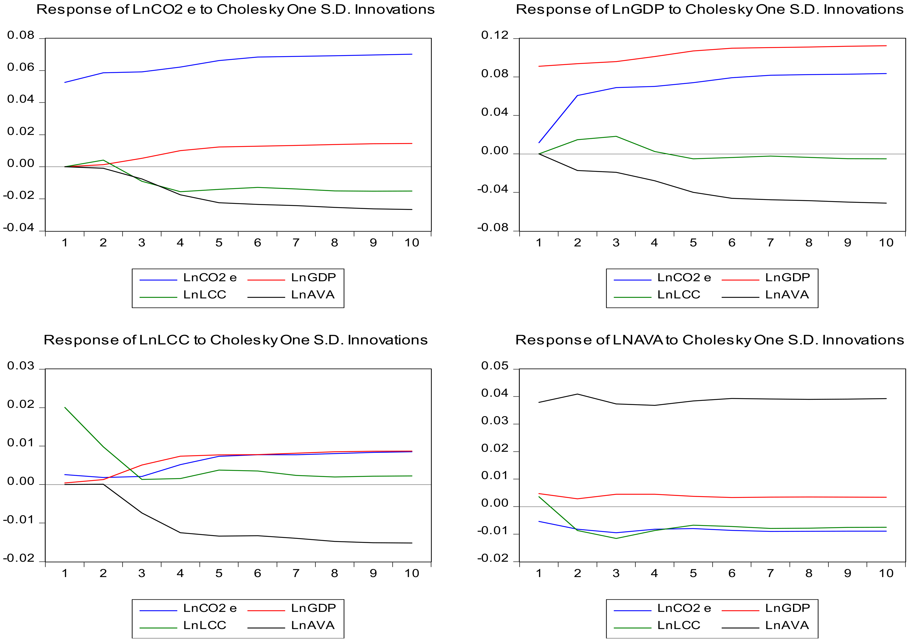
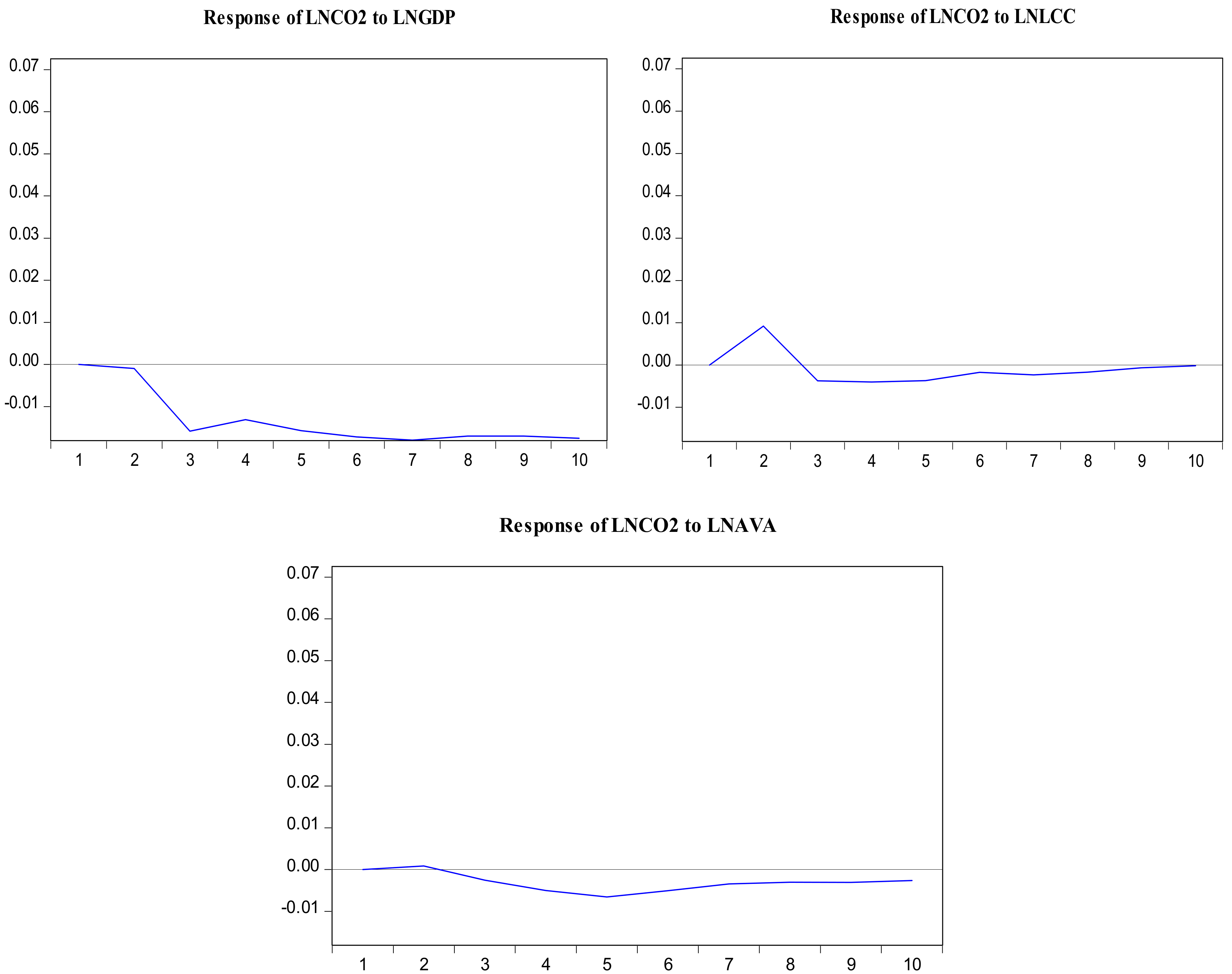
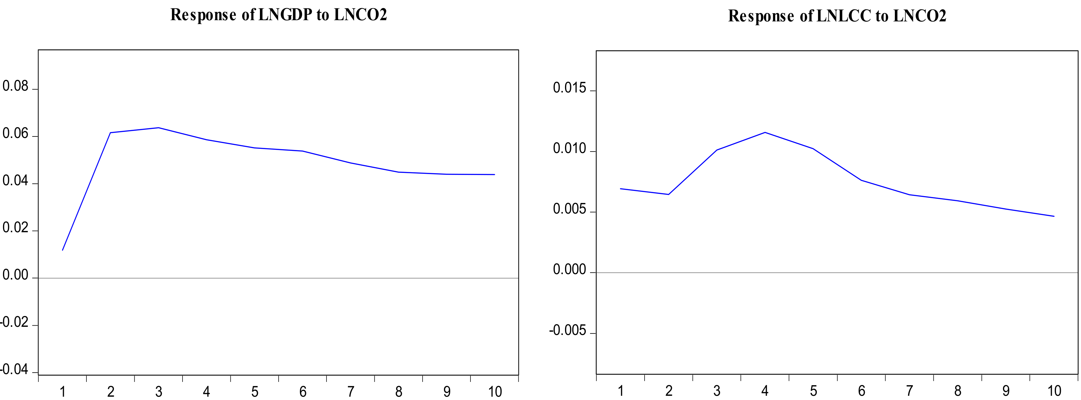
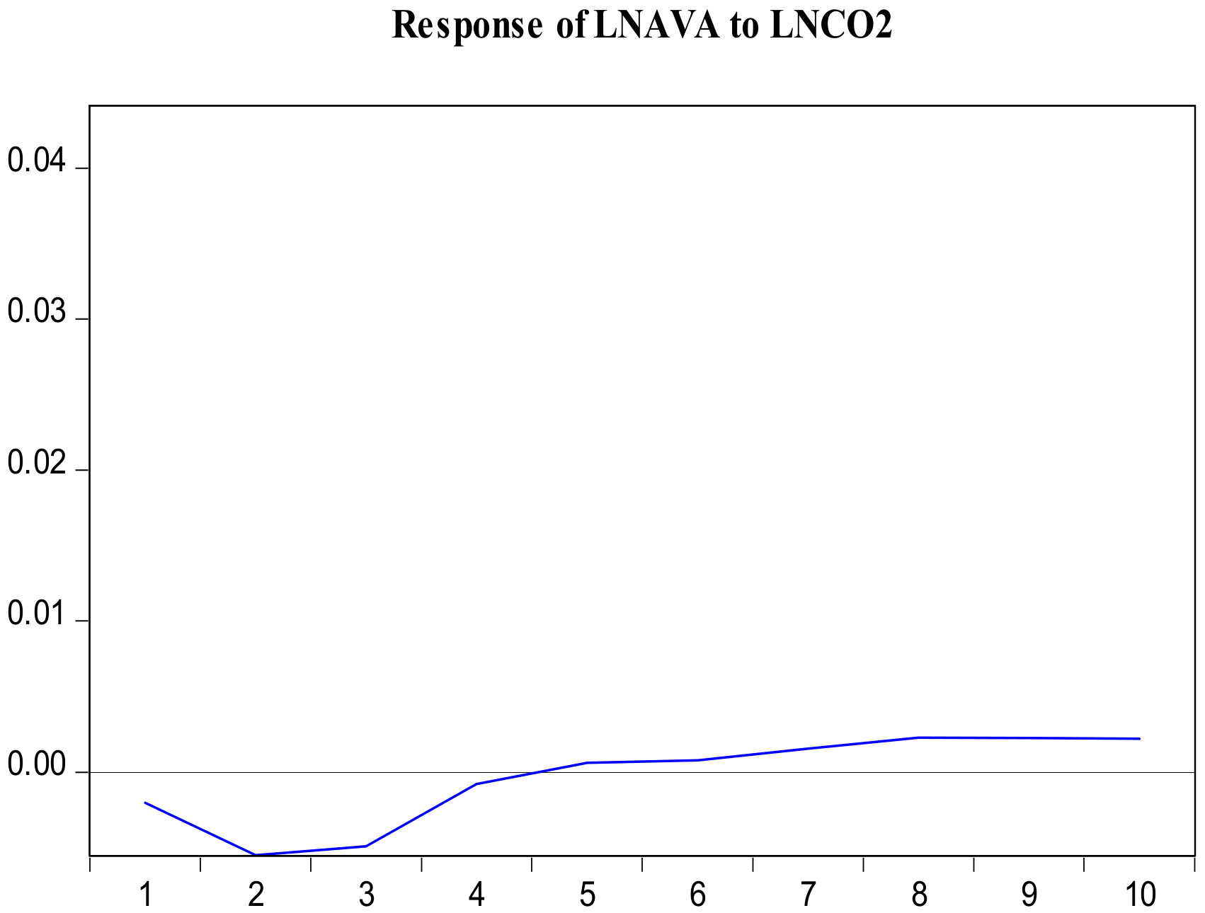
4.9. Impulse Response and Variance Decomposition Analysis

Finally, the study employed impulse response analysis between LnCO₂ e, LnGDP, LnLCC and LnAVA to describe random innovations among them. As the pairwise Granger causality test does not indicate any random response, so in this case, we have to run the impulse response analysis. Figure 6 displays that the response of carbon dioxide emissions to a gross domestic product, land under cereal crops and agriculture value-added are insignificant within 10-period horizons. On the other hand, the initial response of carbon dioxide emissions to land under cereal crop is significant in the beginning. A one standard deviation shock to land under cereal crop first increases carbon dioxide emissions to 1-period horizon and then starts decreasing to the 10-periods horizon. Figure 7 illustrates the response of gross domestic product, land under cereal crop and agricultural value-added to carbon dioxide emissions.

Table 10. Variance decomposition Cholesky ordering; LnCO₂ e_EMISSIONS LnGDP LnLCC LnAVA.

Variance Decomposition of LnCO2 e:
Period	S.E.	LNCO2 e	LnGDP	LnLCC	LnAVA
1	0.052387	100.0000	0.000000	0.000000	0.000000
2	0.082091	98.71976	0.013097	1.256378	0.010761
3	0.110017	97.05350	2.074796	0.812947	0.058761
4	0.131880	96.72981	2.427748	0.658399	0.184048
5	0.151464	96.20375	2.913165	0.557815	0.325269
6	0.168350	95.78747	3.397230	0.461823	0.353472
7	0.183532	95.44742	3.816423	0.404535	0.331620
8	0.197549	95.30147	4.032265	0.356521	0.309743
9	0.210862	95.20442	4.188896	0.313796	0.292891
10	0.223536	95.10645	4.340165	0.279285	0.274097
Variance Decomposition of LnGDP:
Period	S.E.	LnCO2 e	LnGDP	LnLCC	LnAVA
1	0.090540	1.714846	98.28515	0.000000	0.000000
2	0.147440	18.08957	79.94849	0.319798	1.642142
3	0.180273	24.58352	71.58001	0.872488	2.963985
4	0.202225	27.94786	67.03118	1.197606	3.823346
5	0.227024	28.07898	64.92696	1.894400	5.099661
6	0.250104	27.76311	63.32763	2.031381	6.877877
7	0.268642	27.36151	62.39127	2.146152	8.101068
8	0.285511	26.69581	62.00309	2.495791	8.805307
9	0.302657	25.87071	61.89515	2.792302	9.441847
10	0.319132	25.16367	61.79875	2.942672	10.09490
Variance Decomposition of LnLCC:
Period	S.E.	LnCO2 e	LnGDP	LnLCC	LnAVA
1	0.019616	12.45762	0.679255	86.86313	0.000000
2	0.022818	17.21273	0.890578	78.32556	3.571125
3	0.025397	29.76056	3.976938	63.25735	3.005150
4	0.029421	37.65852	8.366014	47.75381	6.221656
5	0.032195	41.56618	7.848681	40.22046	10.36468
6	0.033756	42.90460	7.661578	36.78005	12.65377
7	0.035466	42.15718	8.493156	34.06056	15.28910
8	0.037344	40.54667	9.617245	31.05127	18.78481
9	0.038945	39.10538	10.27839	28.82381	21.79242
10	0.040393	37.68193	10.95538	27.30356	24.05913
Variance Decomposition of LnAVA:
Period	S.E.	LnCO2 e	LnGDP	LnLCC	LnAVA
1	0.040325	0.255478	3.255885	4.319678	92.16896
2	0.060142	0.952231	1.551848	2.327764	95.16816
3	0.071323	1.153774	2.165245	2.590248	94.09073
4	0.081077	0.902385	2.715711	4.100540	92.28136
5	0.091163	0.718266	2.498629	5.149917	91.63319
6	0.100451	0.597671	2.267443	5.312943	91.82194
7	0.108566	0.532349	2.227840	5.480631	91.75918
8	0.116045	0.503706	2.175351	5.836543	91.48440
9	0.123284	0.479624	2.061993	6.111924	91.34646
10	0.130224	0.457998	1.967759	6.249748	91.32449

estimates Cholesky’s method of variance decomposition to random innovation affecting the variables in the VAR [68]. The results indicate that almost 4.3% of the future fluctuations in LnCO₂ e is due to shocks in the LnGDP, 0.27% of future fluctuations in the LnCO₂ e is due to shocks in LnLCC and 0.27% of future fluctuations in the LnCO₂ e is due to shocks in LnAVA, respectively. Evidence from the table shows that almost 25% of future fluctuations in LnGDP is due to shocks in LnCO₂ e, 10% of future fluctuations in LnGDP is due to shocks in LnAVA and 2.9% of future fluctuations in LnGDP is due to shocks in LnLCC. Moreover, evidence from the results shows that almost 37% of future fluctuations in LnLCC is due to shocks in LnCO₂ e, 24% of future fluctuations in LnLCC is due to shocks in LnAVA and 10% of future fluctuations in LnLCC is due to shocks in LnGDP. Finally, the evidence from Table 9 shows that almost 6.2% of the future fluctuations in LnAVA is due to shocks in LnLCC, 1.9% of future fluctuations in LnAVA is due to shocks in LnGDP and 0.4% of future fluctuations in LnAVA is due to shocks in LnCO₂ e, respectively.

5. Conclusions and Policy Recommendations

The purpose of the study was to determine the relationships between CO₂ e as a dependent variable and GDP, LCC and AVA as independent variables in Pakistan. These independent variables have been tested to determine their effect on Pakistan’s carbon dioxide emissions. Therefore, an empirical study was necessary to notify the policymakers and place Pakistan properly in efforts directed to mitigate the consequences of global warming. The study uses time-series data from 1961 to 2014. In the study, we run a descriptive analysis, Johansen co-integration test, pairwise Granger causality test and autoregressive distributed lag model.

The ARDL bounds test co-integration analysis displayed evidence of both short-run and long-run equilibrium relationship between the study variables. The speed of adjustment (ECT) is approximately 7.7 percent in one period of long-run equilibrium. Furthermore, the outcome of CUSUM and CUSUMsq showed that the model used in the study is stable. The pairwise Granger causality test was applied to find out the robustness of the model.

Our study findings have few policy implications for promoting agricultural development. To maintain economic growth and to reduce carbon dioxide emissions, it is very important to adjust and optimize the industrial structure. Pakistan’s industrial sectors are generating heavy and high emissions of carbon dioxide. Therefore, the policymakers need to promote zero and light emissions industries for the development of the country. The results of the study show unidirectional Granger causality from gross domestic product to carbon dioxide emissions which indicates that ensuring a continuous increase in economic growth is a necessary condition for achieving high carbon dioxide emissions. Therefore, the government of Pakistan should take necessary actions to achieve high economic growth with less carbon dioxide emissions. As Pakistan predominantly is an agricultural country, thus, it is summarized that variations in climate change might have negative consequences for agricultural production and industrial growth, poverty reduction and job creation. As a South Asian country, Pakistan is not an exception, and the vulnerability index of climate change in the country is quite high. The country is listed among the countries severely affected by climate change [69] despite being a low producer of CO₂ gases [70] because of its increasing dependence on agriculture for food and fiber needs [71]. In addition, the agriculture sector of Pakistan consists of a majority of small resource, poor farmers with less adaption capacity. For the major crop production of mainly cereals, fruits and vegetables in Pakistan, the policymakers or government need to develop new crop farming methods, introducing new crop varieties, and an extension services role is also very important for spreading the updated science-based information.

References

1. FAO. The State of Food Insecurity in the World the Multiple Dimensions of Food Security; Food and Agriculture Organization of the United Nations: Rome, Italy, 2013. [Google Scholar]
2. Boko, M.; Niang, I.; Nyong, A.; Vogel, A.; Githeko, A.; Medany, M.; Osman-Elasha, B.; Tabo, R.; Yanda Pius, Z. Africa, Climate Change 2007: Impacts, Adaptation and Vulnerability: Contribution of Working Group II to the Fourth Assessment Report of the Intergovernmental Panel on Climate Change; Cambridge University Press: Cambridge, UK, 2007; pp. 433–467. [Google Scholar]
3. Turner, A.G.; Annamalai, H. Climate change and the South Asian summer monsoon. Nat. Clim. Chang. 2012, 2, 587–595. [Google Scholar] [CrossRef]
4. Deressa, T.T.; Hassan, R.M.; Ringler, C. Perception of and adaptation to climate change by farmers in the Nile basin of Ethiopia. J. Agric. Sci. 2011, 149, 23–31. [Google Scholar] [CrossRef] [Green Version]
5. Fatuase, A.; Ajibefun, I. Perception and Adaptation to Climate Change among Farmers in Selected Communities of Ekiti State, Nigeria. Gaziosmanpasa Univ. Ziraat Fak. Derg. 2014, 31, 101–114. [Google Scholar]
6. Gömann, H. How Much did Extreme Weather Events Impact Wheat Yields in Germany?—A Regionally Differentiated Analysis on the Farm Level. Procedia Environ. Sci. 2015, 29, 119–120. [Google Scholar] [CrossRef] [Green Version]
7. Kurukulasuriya, P.; Mendelsohn, R.; Hassan, R.; Benhin, J.; Deressa, T.; Diop, M.; Eid, H.M.; Fosu, K.Y.; Gbetibouo, G.; Jain, S.; et al. Will African agriculture survive climate change? World Bank Econ. Rev. 2006, 20, 367–388. [Google Scholar] [CrossRef] [Green Version]
8. Özdoǧan, M. Modeling the impacts of climate change on wheat yields in Northwestern Turkey. Agric. Ecosyst. Environ. 2011, 141, 1–12. [Google Scholar] [CrossRef]
9. Potgieter, A.; Meinke, H.; Doherty, A.; Sadras, V.O.; Hammer, G.; Crimp, S.; Rodriguez, D. Spatial impact of projected changes in rainfall and temperature on wheat yields in Australia. Clim. Chang. 2013, 117, 163–179. [Google Scholar] [CrossRef]
10. Song, T.; Zheng, T.; Tong, L. An empirical test of the environmental Kuznets curve in China: A panel cointegration approach. China Econ. Rev. 2008, 19, 381–392. [Google Scholar] [CrossRef]
11. Tao, F.; Yokozawa, M.; Xu, Y.; Hayashi, Y.; Zhang, Z. Climate changes and trends in phenology and yields of field crops in China, 1981–2000. Agric. For. Meteorol. 2006, 138, 82–92. [Google Scholar] [CrossRef]
12. Tao, F.; Zhang, S.; Zhang, Z. Spatiotemporal changes of wheat phenology in China under the effects of temperature, day length and cultivar thermal characteristics. Eur. J. Agron. 2012, 43, 201–212. [Google Scholar] [CrossRef]
13. Tao, F.; Zhang, Z.; Xiao, D.P.; Zhang, S.; Rötter, R.P.; Shi, W.J.; Liu, Y.J.; Wang, M.; Liu, F.S.; Zhang, H. Responses of wheat growth and yield to climate change in different climate zones of China, 1981–2009. Agric. For. Meteorol. 2014, 189–190, 91–104. [Google Scholar] [CrossRef]
14. Webb, L.B.; Whetton, P.H.; Barlow, E.W.R. Climate change and winegrape quality in Australia. Clim. Res. 2008, 36, 99–111. [Google Scholar] [CrossRef]
15. You, L.; Rosegrant, M.W.; Wood, S.; Sun, D. Impact of growing season temperature on wheat productivity in China. Agric. For. Meteorol. 2009, 149, 1009–1014. [Google Scholar] [CrossRef]
16. Ahmad, M.; Farooq, U. The state of food security in Pakistan: Future challenges and coping strategies. Pak. Dev. Rev. 2010, 49, 903–923. [Google Scholar] [CrossRef] [Green Version]
17. Kang, Y.; Khan, S.; Ma, X. Climate change impacts on crop yield, crop water productivity and food security—A review. Prog. Nat. Sci. 2009, 19, 1665–1674. [Google Scholar] [CrossRef]
18. IPCC. Climate Change 2014: Synthesis Report. Contribution of Working Groups I, II and III to the Fifth Assessment Report of the Intergovernmental Panel on Climate Change; IPCC: Geneva, Switzerland, 2014.
19. Stocker, T.F.; Qin, D.; Plattner, G.K.; Tignor, M.M.B.; Allen, S.K.; Boschung, J.; Nauels, A.; Xia, Y.; Bex, V.; Midgley, P.M. IPCC, 2013: Climate Change 2013: The Physical Science Basis. Contribution of Working Group I to the Fifth Assessment Report of the Intergovernmental Panel on Climate Change; IPCC: Geneva, Switzerland, 2013; p. 1535. [Google Scholar]
20. Gorst, A.; Groom, B.; Dehlavi, A. Crop Productivity and Adaptation to Climate Change in Pakistan Centre for Climate Change. Environ. Dev. Econom. 2018, 23, 1–23. [Google Scholar] [CrossRef] [Green Version]
21. Sönke, K.; Eckstein, D.; Dorsch, L.; Fischer, L. Global Climate Risk Index 2016: Who Suffers most from Extreme Weather Events? Weather-Related Loss Events in 2014 and 1995 to 2014; Report from Germanwatch; Germanwatch: Bonn, Germany, 2015; pp. 1–28. Available online: https://germanwatch.org/sites/germanwatch.org/files/publication/16411.pdf (accessed on 30 October 2019).
22. Abid, M.; Scheffran, J.; Schneider, U.A.; Ashfaq, M. Farmers’ perceptions of and adaptation strategies to climate change and their determinants: The case of Punjab province, Pakistan. Earth Syst. Dyn. 2015, 6, 225–243. [Google Scholar] [CrossRef] [Green Version]
23. Tunç, G.I.; Türüt-Aşık, S.; Akbostancı, E. A decomposition analysis of CO2 emissions from energy use: Turkish case. Energy Policy 2009, 37, 4689–4699. [Google Scholar] [CrossRef]
24. Sarkar, M.S.K.; Sadeka, S.; Sikdar, M.M.H.; Zaman, B. Energy Consumption And CO2 Emission In Bangladesh: Trends And Policy. Asia Pac. J. Energy Environ. 2015, 2, 175–182. [Google Scholar] [CrossRef]
25. Appiah, K.; Dua, J.; Boamah, K.B. The Effect of Environmental Performance on Firm’s Performance—Evidence from Ghana. Br. J. Interdiscip. Res. 2017, 8, 340–348. [Google Scholar]
26. Appiah, K.; Du, J.; Musah, A.A.I.; Afriyie, S. Investigation of the Relationship between Economic Growth and Carbon Dioxide (CO2) Emissions as Economic Structure Changes: Evidence from Ghana. Resour. Environ. 2017, 7, 160–167. [Google Scholar]
27. McAusland, C. Globalisation’s Direct and Indirect Effects on the Environment. Glob. Transp. Environ. 2010, 31–53. [Google Scholar] [CrossRef]
28. Adom, P.K.; Bekoe, W.; Amuakwa-mensah, F.; Mensah, J.T.; Botchway, E. Carbon dioxide emissions, economic growth, industrial structure, and technical efficiency: Empirical evidence from Ghana, Senegal, and Morocco on the causal dynamics. Energy 2012, 47, 314–325. [Google Scholar] [CrossRef]
29. Asumadu-Sarkodie, S.; Owusu, P.A. The relationship between carbon dioxide and agriculture in Ghana: A comparison of VECM and ARDL model. Environ. Sci. Pollut. Res. 2016, 23, 10968–10982. [Google Scholar] [CrossRef] [PubMed]
30. Shahbaz, M.; Khan, S.; Ali, A.; Bhattacharya, M. The impact of globalization on CO2 emissions in china. Singap. Econ. Rev. 2017, 62, 929–957. [Google Scholar] [CrossRef] [Green Version]
31. Pesaran, M.H.; Shin, Y. An autoregressive distributed-lag modelling approach to cointegration analysis. Econom. Soc. Monogr. 1998, 31, 371–413. [Google Scholar]
32. Gokmenoglu, K.K.; Taspinar, N. Testing the agriculture-induced EKC hypothesis: The case of Pakistan. Environ. Sci. Pollut. Res. 2018, 25, 22829–22841. [Google Scholar] [CrossRef]
33. Liu, X.; Zhang, S.; Bae, J. The impact of renewable energy and agriculture on carbon dioxide emissions: Investigating the environmental Kuznets curve in four selected ASEAN countries. J. Clean. Prod. 2017, 164, 1239–1247. [Google Scholar] [CrossRef]
34. Asumadu-sarkodie, S.; Owusu, P.A.; Asumadu-sarkodie, S.; Owusu, P.A. Carbon dioxide emission, electricity consumption, industrialization, and economic growth nexus: The Beninese case. Energy Sources Part B Econ. Plan. Policy 2016, 11, 1089–1096. [Google Scholar] [CrossRef]
35. Asumadu-Sarkodie, S. Carbon dioxide emissions, GDP, energy use, and population growth: A multivariate and causality analysis for Ghana, 1971–2013. Environ. Sci. Pollut. Res. 2016, 23, 13508–13520. [Google Scholar] [CrossRef]
36. Zhang, L.; Pang, J.; Chen, X.; Lu, Z. Carbon emissions, energy consumption and economic growth: Evidence from the agricultural sector of China’s main grain-producing areas. Sci. Total Environ. 2019, 665, 1017–1025. [Google Scholar] [CrossRef] [PubMed]
37. Zafeiriou, E.; Azam, M. CO2 emissions and economic performance in EU agriculture: Some evidence from Mediterranean countries. Ecol. Indic. 2017, 81, 104–114. [Google Scholar] [CrossRef]
38. Gornall, J.; Betts, R.; Burke, E.; Clark, R.; Camp, J.; Willett, K.; Wiltshire, A. Implications of climate change for agricultural productivity in the early twenty-first century. Philos. Trans. R. Soc. B. Biol. Sci. 2010, 365, 2973–2989. [Google Scholar] [CrossRef] [PubMed]
39. Victor, P.A. Growth, degrowth and climate change: A scenario analysis. Ecol. Econ. 2012, 84, 206–212. [Google Scholar] [CrossRef]
40. Barrios, S.; Ouattara, B.; Strobl, E. The impact of climatic change on agricultural production: Is it different for Africa? Food Policy 2008, 33, 287–298. [Google Scholar] [CrossRef] [Green Version]
41. Ayinde, O.E.; Muchie, M.; Olatunji, G.B. Effect of Climate Change on Agricultural Productivity in Nigeria: A Co-integration Model Approach. J. Hum. Ecol. 2011, 35, 189–194. [Google Scholar] [CrossRef]
42. Chen, J.; Cheng, S.; Song, M. Changes in energy-related carbon dioxide emissions of the agricultural sector in China from 2005 to 2013. Renew. Sustain. Energy Rev. 2018, 94, 748–761. [Google Scholar] [CrossRef]
43. Goklany, I.M. Integrated strategies to reduce vulnerability and advance adaptation, mitigation, and sustainable development. Mitig. Adapt. Strateg. Glob. Chang. 2007, 12, 755–786. [Google Scholar] [CrossRef]
44. Tol, R.S.J.; Downing, T.E.; Kuik, O.J.; Smith, J.B. Distributional aspects of climate change impacts. Glob. Environ. Chang. 2004, 14, 259–272. [Google Scholar] [CrossRef]
45. Li, W.; Ou, Q.; Chen, Y. Decomposition of China’s CO2 emissions from agriculture utilizing an improved Kaya identity. Environ. Sci. Pollut. Res. 2014, 21, 13000–13006. [Google Scholar] [CrossRef]
46. Ismael, M.; Srouji, F.; Boutabba, M.A. Agricultural technologies and carbon emissions: Evidence from Jordanian economy. Environ. Sci. Pollut. Res. 2018, 25, 10867–10877. [Google Scholar] [CrossRef] [PubMed]
47. Dickey, D.A.; Fuller, W.A. Likelihood Ratio Statistics For Autoregressive Time Series With A Unit. Econometrica 1981, 49, 1057–1072. [Google Scholar] [CrossRef]
48. Phillips, P.; Perron, P. Testing for a unit root in time series regression. Biometrika 1988, 75, 335–346. [Google Scholar] [CrossRef]
49. Akalke, H. A New Look at the Statistical Model Identification. IEEE Trans. Autom. Control 1974, 19, 716–723. [Google Scholar]
50. Schwarz, G. Institute of Mathematical Statistics is collaborating with JSTOR to digitize, preserve, and extend access to The Annals of Statistics. Ann. Stat. 1978, 6, 461–464. [Google Scholar] [CrossRef]
51. Khim, V.; Liew, S. Which Lag Length Selection Criteria Should We Employ? Econ. Bull. 2004, 3, 1–9. [Google Scholar]
52. Johansen, S. Statistical Analysis of Cointegration Vectors. J. Econ. Dyn. Control 1988, 12, 231–254. [Google Scholar] [CrossRef]
53. Johansen, S.; Juselius, K. Maximum Likelihood Estimation and Inference on Cointegration—With applications to the demand for money. Oxf. Bull. Econ. Stat. 1990, 52, 169–210. [Google Scholar] [CrossRef]
54. Pesaran, M.H.; Shin, Y.; Smith, R.J. Bounds testing approaches to the analysis of level relationships. J. Appl. Econom. 2001, 16, 289–326. [Google Scholar] [CrossRef]
55. Boutabba, M.A. The impact of fi nancial development, income, energy and trade on carbon emissions: Evidence from the Indian economy. Econ. Model. 2014, 40, 33–41. [Google Scholar] [CrossRef] [Green Version]
56. Shahbaz, M.; Hooi, H.; Shahbaz, M. Environmental Kuznets Curve hypothesis in Pakistan: Cointegration and Granger causality. Renew. Sustain. Energy Rev. 2012, 16, 2947–2953. [Google Scholar] [CrossRef] [Green Version]
57. Ozturk, I.; Acaravci, A. The long-run and causal analysis of energy, growth, openness and fi nancial development on carbon emissions in Turkey. Energy Econ. 2013, 36, 262–267. [Google Scholar] [CrossRef]
58. Hooi, H.; Smyth, R. CO2 emissions, electricity consumption and output in ASEAN. Appl. Energy 2010, 87, 1858–1864. [Google Scholar]
59. Fodha, M.; Zaghdoud, O. Economic growth and pollutant emissions in Tunisia: An empirical analysis of the environmental Kuznets curve. Energy Policy 2010, 38, 1150–1156. [Google Scholar] [CrossRef]
60. Ferda, H. An econometric study of CO2 emissions, energy consumption, income and foreign trade in Turkey. Energy Policy 2009, 37, 1156–1164. [Google Scholar]
61. Kanjilal, K.; Ghosh, S. Environmental Kuznet’s curve for India: Evidence from tests for cointegration with unknown structural breaks. Energy Policy 2013, 56, 509–515. [Google Scholar] [CrossRef]
62. Jayanthakumaran, K.; Verma, R.; Liu, Y. CO2 emissions, energy consumption, trade and income: A comparative analysis of China and India. Energy Policy 2012, 42, 450–460. [Google Scholar] [CrossRef]
63. Jalil, A.; Mahmud, S.F. Environment Kuznets curve for CO2 emissions: A cointegration analysis for China. Energy Policy 2009, 37, 5167–5172. [Google Scholar] [CrossRef] [Green Version]
64. Lotfalipour, M.R.; Falahi, M.A.; Ashena, M. Economic growth, CO2 emissions, and fossil fuels consumption in Iran. Energy 2010, 35, 5115–5120. [Google Scholar] [CrossRef]
65. Nasir, M.; Rehman, F.U. Environmental Kuznets Curve for carbon emissions in Pakistan: An empirical investigation. Energy Policy 2011, 39, 1857–1864. [Google Scholar] [CrossRef]
66. Saboori, B.; Sulaiman, J.; Mohd, S. Economic growth and CO2 emissions in Malaysia: A cointegration analysis of the Environmental Kuznets Curve. Energy Policy 2012, 51, 184–191. [Google Scholar] [CrossRef]
67. Brown, R.L.; Durbin, J.; Evans, J.M. Techniques for testing the constancy of regression relationships over time. J. R. Stat. Soc. Ser. B 1975, 37, 149–192. [Google Scholar] [CrossRef]
68. Payne, J.E. Inflationary dynamics of a transition economy: The Croatian experience. J. Policy Model. 2002, 24, 219–230. [Google Scholar] [CrossRef] [Green Version]
69. Smadja, J.; Aubriot, O.; Puschiasis, O.; Duplan, T.; Hugonnet, M. Climate change and water resources in the Himalayas: Field study in four geographic units of the Koshi. J. Alp. Res. 2015, 103, 2–22. [Google Scholar] [CrossRef] [Green Version]
70. Yousuf, I.; Ghumman, A.R.; Hashmi, H.N.; Kamal, M.A. Carbon emissions from power sector in Pakistan and opportunities to mitigate those. Renew. Sustain. Energy Rev. 2014, 34, 71–77. [Google Scholar] [CrossRef]
71. Ahmad, M.; Mustafa, G.; Iqbal, M. Impact of Farm Households’ Adaptations to Climate Change on Food Security: Evidence from Different Agro-Ecologies of Pakistan. Pakistan development review. 2016, 55, 561–588. [Google Scholar]
Figure 1. Trend of the study variables.
Energies 12 04590 g001aEnergies 12 04590 g001b
Figure 2. ARDL model selection criterion. Source. Authors’ calculation.
Energies 12 04590 g002
Figure 3. Results of generalized impulse response functions.
Energies 12 04590 g003
Figure 4. Stability test based on (a) cumulative sum of the recursive residuals (CUSUM) and (b) CUSUM of squares. Source. Authors’ calculation.
Energies 12 04590 g004
Figure 5. Checking the stability of vector autoregression (VAR).
Energies 12 04590 g005
Figure 6. Impulse response of LnCO2 e to Cholesky one standard deviation (S.D.).
Energies 12 04590 g006
Figure 7. Impulse-response of other variables to Cholesky one S.D. Innovations in LnCO2 e.
Energies 12 04590 g007aEnergies 12 04590 g007b