Article

Theoretical and Experimental Study to Determine Voltage Violation, Reverse Electric Current and Losses in Prosumers Connected to Low-Voltage Power Grid

by
Igor Cavalcante Torres
1,*,
Gustavo F. Negreiros
2 and
Chigueru Tiba
2
1
Agricultural Sciences Center, Universidade Federal de Alagoas, Rio Largo 57100-000, Brazil
2
Nuclear Energy, Universidade Federal de Pernambuco, Recife 50740-545, Brazil
*
Author to whom correspondence should be addressed.
Energies 2019, 12(23), 4568; https://doi.org/10.3390/en12234568
Submission received: 28 October 2019 / Revised: 19 November 2019 / Accepted: 26 November 2019 / Published: 29 November 2019
(This article belongs to the Special Issue Integration of PV in Distribution Networks)

Abstract

:
The impact of PV generation distributed in a low voltage transmission line depends on many factors: The distribution lines and PV generators characteristics, its location, operational control, local meteorological conditions, electricity consumption profile, and the electricity cost variation. An atypical and challenging behavior of photovoltaic distributed generation (DG) insertion in consumer units (CUs), implies in some circumstances, as the reverse directionality of the power flow between the load equipped with a photovoltaic system generator and the electrical grid, when a CU contains a distributed generation and low power consumption, the power flow will be directed to the power electric grid. In this work, the modeling of a low-voltage real feeder was performed, setting the variables of the system under real operating conditions. As result, voltage levels variability throughout the feeder, the electrical losses, and the asymmetry between the phases were observed. Through simulation scenarios, the occurrence of voltage increase under different penetration scenarios of distributed generation was verified and there was a 10% increase in reference voltage as well as the occurrence of higher electrical losses by reverse current, reaching 1200% more with a DG penetration, in the massive presence of the photovoltaic generator. The mitigatory action used in this work was able to attenuate the negative impacts to the feeder circuit, ensuring the integrity grid and the consumer unit.

1. Introduction

Nowadays, the technological advance increasingly demands electricity to supply its needs, whether at a residential, industrial, or commercial level. Even with the environmental awareness and efforts to rationalize the use of electricity, there is a strong growth of electronic equipment, such as cellphones, televisions, air conditioning, and others in urban environments. Energy complementarity is a way of aggregating power from different sources to the electrical matrix, supplying the demand on moments of scarcity. Photovoltaic solar energy emerges as one of the options to mitigate this problem [1]. The development of this energetic modality in Brazil occurred with the creation of the Resolution 414/2012, added and renumbered to 687/2015, along with the creation of module 8 of distribution procedure. These two normative documents are responsible for regulating energy insertion, generation of electricity connected to the network, and monitoring the quality of the electricity [2]. Due to this standardization process and to the enormous potential for solar resource utilization in Brazil, in the year 2017, from the 10,561 connections performed until the month of May of that year [3], 10,453 came from photovoltaic solar source, which when compared to other generation sources, represented 99% of the number of installations. In function of a significant network insertion of intermittent nature sources, such as PV, researchers are arousing interest in reanalyzing the load flow study, especially in the low-voltage networks, where the penetration of microgeneration tends to be more aggressive. As a consequence of the large number of distributed generation connections in low voltage feeders, several stability problems emerge in the network, such as reverse power flow in the line sections and in transformers, unexpected voltage increase in the load bars, occasional islanding, and flicker effect [4]. The lack of complete automation of the distribution system, especially in the consumer units, makes it a challenging task [5], since the high power supplied associated with a demand curve raises the superior limits of electric voltage even more.
Chathurangi D. et al. [6] presented results concerning relevant impacts on electrical quality in the low voltage distribution networks with high levels of photovoltaic systems penetration, and highlighted the necessity of planning for mitigating solutions. M. J. Reno et al. [7] studied the presence of distributed generation in the current electrical system and how this expressively influences in the power flow and highlighting the damaging aspects to the system. Silva Júnior, S. B. [5] presented a computational analysis, from the OPENDSS-EPRI software, for the behavior verification of an electricity distribution, taking into consideration all the real aspects of operation. Chiconi, D. N. [8] performed a modeling in the OPENDSS-EPRI of a low voltage feeder, comparing it with the presence or absence of a PV generator of 15 kW. Voltage data in the busbar, power flow, and energy quality parameters were presented aiming to further improve these parameters. De Carne. et al. [9] demonstrated that a high injection of energy from low-voltage distributed generation, induces a reverse flow reaching the primary side of the transformer up to the point of connection to the medium voltage power grid.
All the authors mentioned point out that as the solar energy takes larger proportions in the network in comparison to other generation sources of electricity, it is becoming increasingly important to be aware of the new technical challenges to be faced, especially regarding stability and reliability. The insertion of photovoltaic systems to the electricity distribution feeder causes thresholds or operational phenomena unpredicted previously, violating the stablished normative standards [10,11].
In Brazil, the current standardization predicts that the photovoltaic system is dimensioned to potentially delivery all the generated production and, with that, the technical problems worsen even more, since the initial conception of the power networks, in most cases, may not bear the installed potential of generation, even if they are compatible with the requirements established by the normative resolution [12,13]. Given this fact, this article approached a study based on a section of a real feeder of electricity distribution, situated in the city of Maceió-AL, modeled within the OPENDSS-EPRI open source environment, determining a realistic simulation scenario. The study simulated the load flow in single-family residential consumer unit (CU) highlighting the voltage profile throughout one day, considering the maximum load of the photovoltaic systems. A verification test was performed from a completely instrumented CU, collecting instant information of weather and electrical data, with which it was possible to make a detailed comparison between simulation and reality. In the problem formulation, a flowchart was presented with a methodological procedure that can be used by the power distributors, to ensure the level of reliable and safe penetration of DG to the current electric power system (EPS). Given the current context of the electric utilities in Brazil, this work is of fundamental importance to make them more rigorous in granting permission to new accessors to the power grid that aim energy sharing.

2. Problems Caused by Photovoltaic Generators to the Voltage of Power Grid

2.1. Operating Conditions of an Electricity Distributor Feeder

An energy supply system must ensure the quality and the reliability of electricity, fundamentally respecting the limits of electrical voltage. Voltage in a permanent regime must be tracked throughout the entire distribution system, because the electrical equipment for domestic use can suffer damage when such values exceed the allowed limits [14]. The normative conditions are detailed in Table 1 below [14,15].
The data mentioned in the table above also refer to the type of service extension of the consumer unit (CU), that in turn depends on the installed demand in the residence; therefore, Table 2 associates the relation between installed power and service voltage.
The values shown in Table 2 vary according to the regions and the electrical utilities. The data mentioned in the respective table came from the local electrical utility regulations [14]. The penetration of distributed generation (DG) was conditioned to the limits of power established by local regulation of the electricity company [15], where each DG may vary the power up to the one-phase maximum limit P ≤ 15 kW (100%).

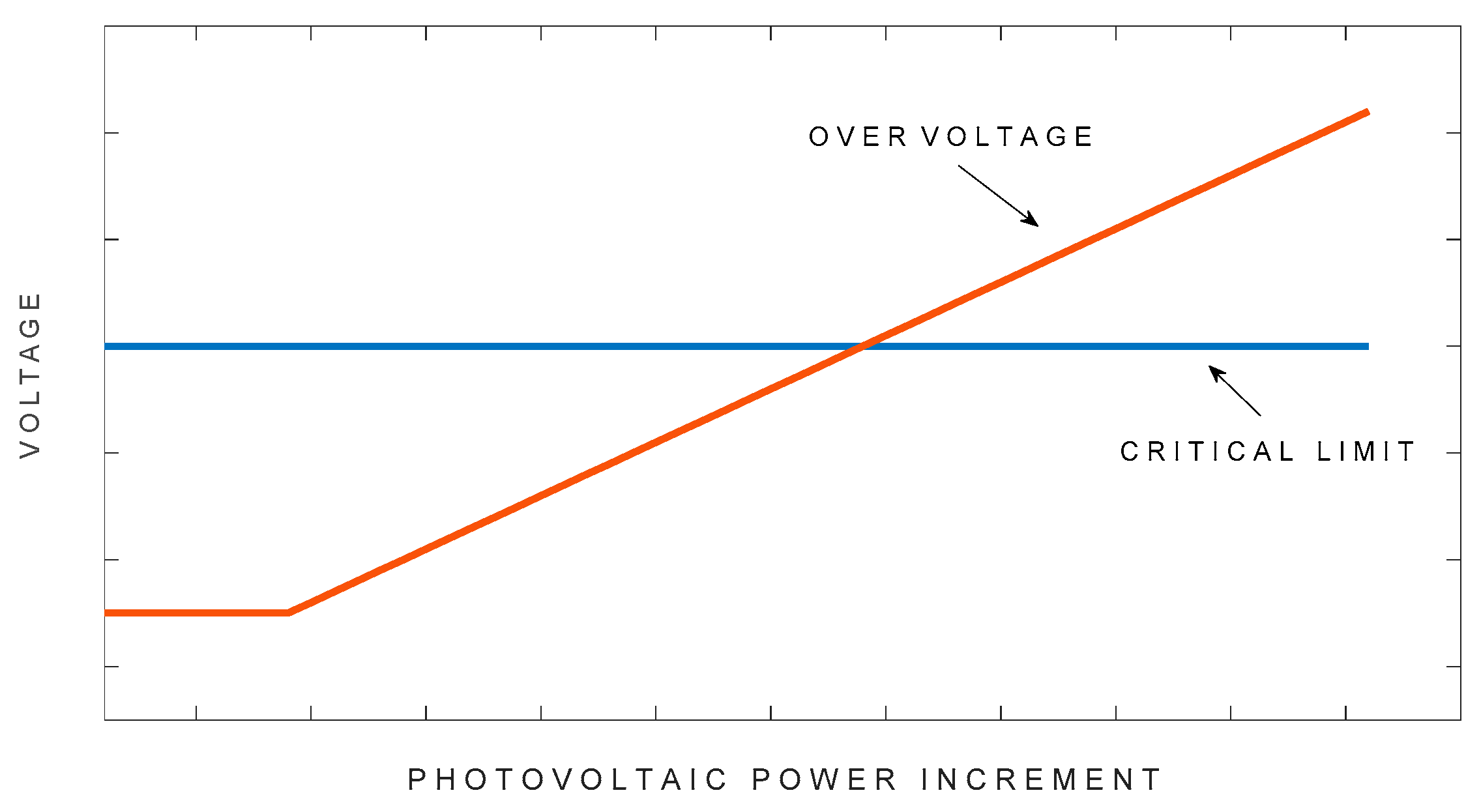
2.2. Influence of Photovoltaic Systems in the Voltage of a CU

The electric power distribution system was initially conceived to deliver power to a consumer radially. With the creation of the normative resolution 687/2015 from the National Electric Energy Agency (ANEEL), the point of view regarding electricity consumers is under new definition, classifying a CU as an electricity prosumer, which ensures that it goes on to produce locally its own electricity [2]. Through the illustrations in Figure 1a, it is possible to visualize the unidirectional flow dynamics (conventional) and in Figure 1b, the reverse flow in a generic section of a feeder.
The images simplify the connection of multiple CUs to a feeder knot ( V 2 ) through the extension impedance Z 2 n . The section impedance, Z L 1 , interconnects the bars to the distribution substation. Depending on the type of feeder, the line impedance ( Z L 1 ) and the service extension impedance are represented as active and reactive components (R + jX), characterized by the cable type and the total distance of the network section. Similarly, the demand ( P UC ) and photovoltaic generators ( P PV ) are represented by the complex power given by S = P + jQ . The direction of the current flow ( I 2 n ) is variable, changing its direction when there is a photovoltaic generator in the CUs. When P PV = 0 , there is a voltage drop in the service extension ( V sn ) given by Equation (1).
V sn = i 2 n · Z sn = i 2 n · ( r sn + jx sn ) = V rn + jV xn
When P PV P UC , a power in reverse direction will emerge by the impedance Z sn , the current flowing through the section is adopted as I 2 n ; from that, Equation (2) is obtained considering the voltage module on the side of the CU.
V sn = i 2 n · Z sn = i 2 n · ( r sn + jx sn ) = P PV V 2 n · r sn + Q UC V 2 n · x sn
The negative sign in the first portion merely indicates that the increase of voltage will occur on the side of the consumer. Inserting the real component of Equation (2) in the respective term of Equation (3a), it is possible to calculate the voltage value in the side of the consumer when the power supplied by the photovoltaic system exceeds the local demand.
V 2 n = V 2 V sn = V 2 ( P PV V 2 n · r sn )
Analyzing Equation (3a), considering that the demand profile is constant throughout the day, too much power increase from the photovoltaic generator will inevitably cause an increase in the voltage on the load bar. The phenomenon mentioned can be seen in Figure 2.
Figure 2 illustrates voltage behavior in a low voltage service extension, the occurrence of overvoltage due to the excess of reverse power flow, and structural physical conditions of the electrical circuit. The voltage rise may spread throughout the feeder in case more DGs are connected to the main knot of the feeder, as well as if the weather conditions are favorable to overcome nominal values of photovoltaic generators.

3. Data Collection for Feeder Modeling and Simulation

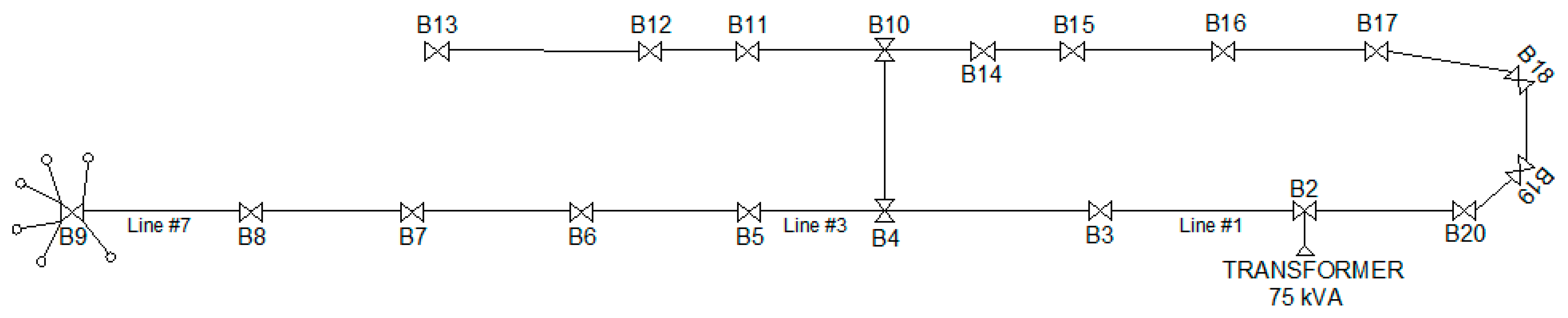
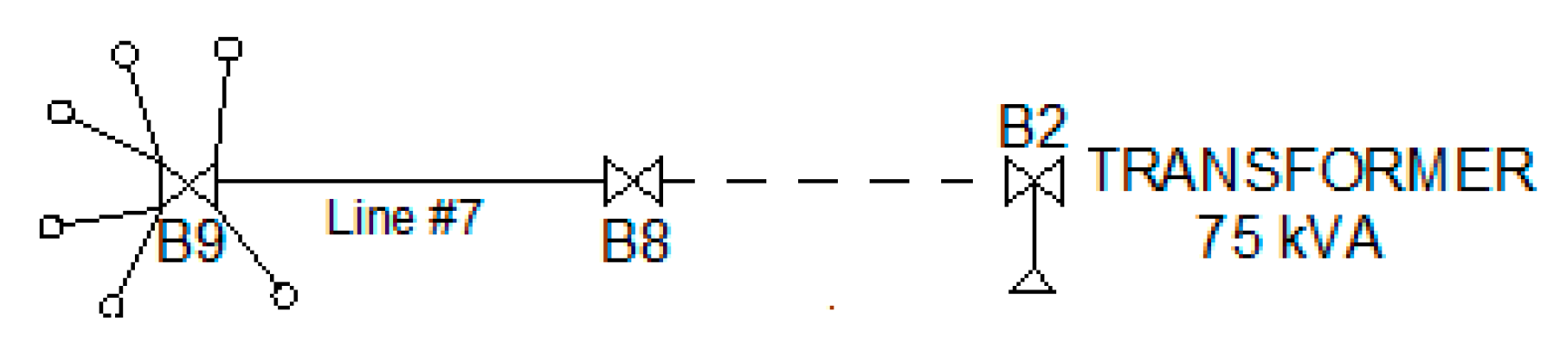
3.1. Real Feeder Identification

A low-voltage distribution system can operate with levels of three-phase 380 V and one-phase 220 V, and commonly presents an aerial topology consisting in bars and conductors, carrying power to four wires in the three-phase star model, when there is double voltage. Circuit energization is conditioned to a substation with primary feeding of 13,800 V in the delta module and maximum power of 75 kVA. Figure 3 below illustrates a real feeder.
The distribution lines were modeled taking into consideration the layout and real characteristics of the cables and spacing between the bars (all raised in the field), and so the nodal admittance matrices were defined from the information of their sequential impedance, resistance, and reactance. The standardization of bars and section of the network was declared in one of the subroutines from the main script of the code. Geometry modeling of the sustaining structures and isolation of the conductors follows references found in the regulation of the local energy distributor [16]. The feeder supplies energy to 202 residential consumers, distributed in the 20 bars of the system, where 189 are connected to the one-phase circuit and the others connected to the three-phase circuit.

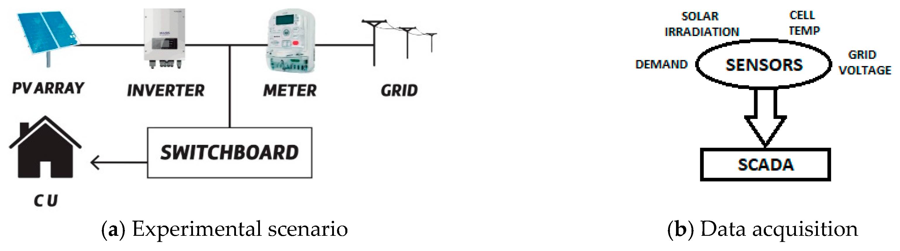
3.2. Simulation Data Acquisition

Monitoring PV plants is an urgent activity for practical implementation due to the information that allows owners to maintain, operate, and control these systems. The work done by Beránek [17] focuses on designing and testing a unique monitoring system with third-generation software for photovoltaic arrays.
Simulation standardization was performed in the OPENDSS environment in temporal mode. In this work, there was the concern to visualize the voltage behavior at the service extension of a consumer unit (CU) facing the insertion of photovoltaic generators, in order to confront tolerance limits pre-established by regulation. For that, a residence located in the feeder at a final section of the network (section 08) was considered, at the last bar (B9), properly instrumented and with data acquisition system (SCADA). Through the SCADA records, it was possible to determine the input profiles for the simulation. Figure 4 illustrates the composition of the experimental environment, as well as the layout of the instrumentation used.
The power systems elements used in OPENDSS, such as PVSystem and Load, presented models that used the monitored variable illustrated in Figure 4b as input values. Data acquisition was adjusted to register data every one minute, enabling the assembling of the solar irradiation loadshapes, demand, and operating temperature of the photovoltaic module.

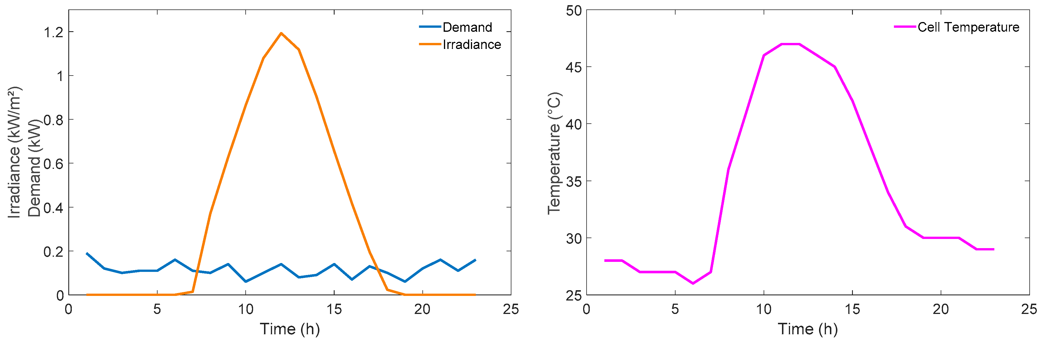
3.2.1. Solar Irradiance Data and Operating Temperature of PV Panel

The energy quality from the photovoltaic systems is closely linked to the quantity of incident solar energy on the PV panels surface, the operating temperature of the cell, and panel efficiency. The PV System element of the OPENDSS requires irradiance and panel temperature input data as input quantities in its mathematical model to estimate daily electrical power delivered to the power system to which it is connected. The solar irradiation profile was collected through a pyranometer and a temperature sensor installed together to the photovoltaic modules, both connected to the Scientific Campbell CR1000 datalogger.
Irradiation and temperature loadshapes operate together with the basis quantities of irradiation and operating temperature of the cell, being adopted in such quantities as 1 kW/m2 and 25 °C, respectively.

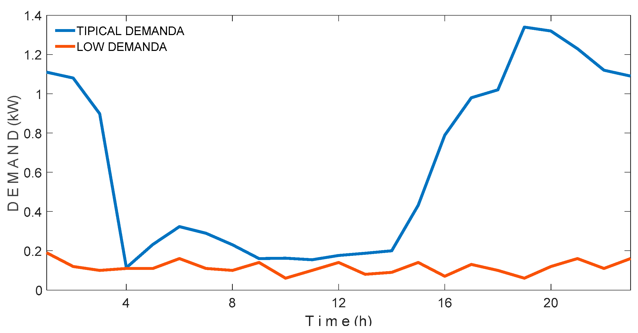
3.2.2. Demand Curves Acquisition

The power distribution system studied supplies 202 CUs, framed as residential consumers, being 83% of the clients connected to the one-phase circuit. The load curves adopted were obtained from a demand monitor, manufacturer ISSO and reference DMI P100. For simulation purposes, two load curves from consumer units linked to the busbar 09, shown previously in Figure 3, were measured. Characteristically, the feeder is besieged by single-family residences, where during most of the day, the load curve operates in region of minimal demand. Figure 5 presents two demand profiles, framed in active power.
Taking as reference the curves from the graph above, there are two particular situations that are commonly attributed to residential loads. Reflecting the blue curve to a real situation, it is characterized as a field house, eventually occupied. The brown curve presents an urban behavior, where the demand peaks occur at night. It is important to stress that both demands can belong to a single family group and, fostered by normative resolution 482/2012 ANEEL, local power use can be contemplated by a distributed generation installed remotely in another CU.

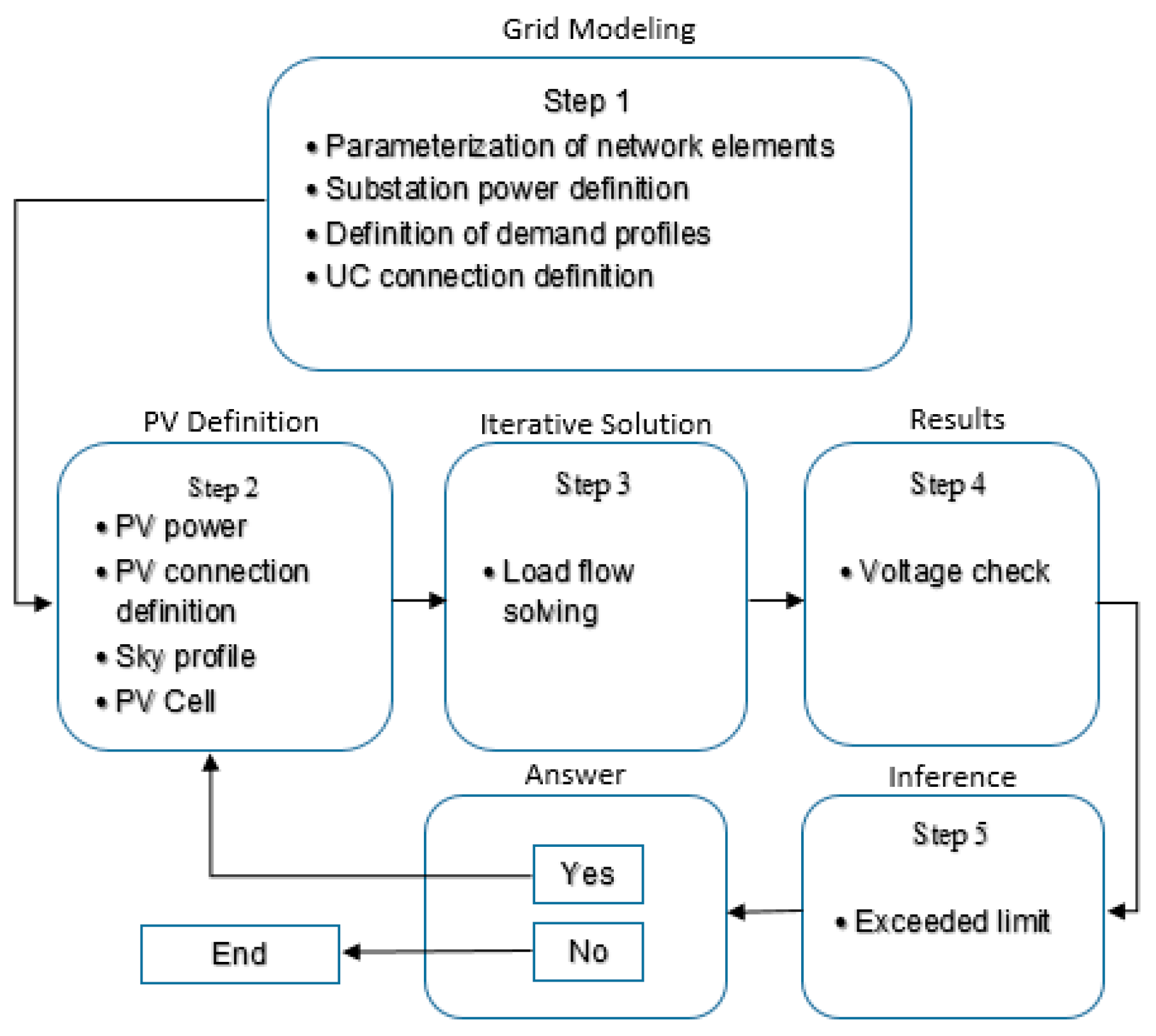
4. Problem Formulation and Methodology

For the study of power flow in distribution networks, the combination of four variables referenced in Table 3 was performed, where two of them are input parameters and the other two incognitos. The bars types definitions are also present, as well as their identification in the studied feeder.
The load flow calculation involves determining the state of the network and consists on knowing the behavior in permanent regime based on the fundamental frequency, bars voltages, currents, and power injected in the elements. Traditionally, power flow calculation for transmission networks is based on interactive numerical methods such as Newton–Raphson and Gaus–Seidel; however, when reflected in the distribution feeders, these devices lose effectiveness due to mesh operation, high R/X (Resistance/Reactance) ratio, and imbalance [18]. To perform the simulation, it is necessary to name the bars; when there are load bars, it is called bar PQ (active power and reactive power); for a source bar or reference, we assign the bar Vθ (voltage module and voltage angle). The simulation performed in this article will be developed in the OPENDSS-EPRI open source environment, where the network modeling is based on the feeder nodal admittance matrix, and can be seen in Equation (3b).
[ V 1 V 2 V 3 ] = [ Y 11 Y 12 Y 13 Y 21 Y 22 Y 23 Y 31 Y 32 Y 33 ] x   [ I 1 I 2 I 3 ]

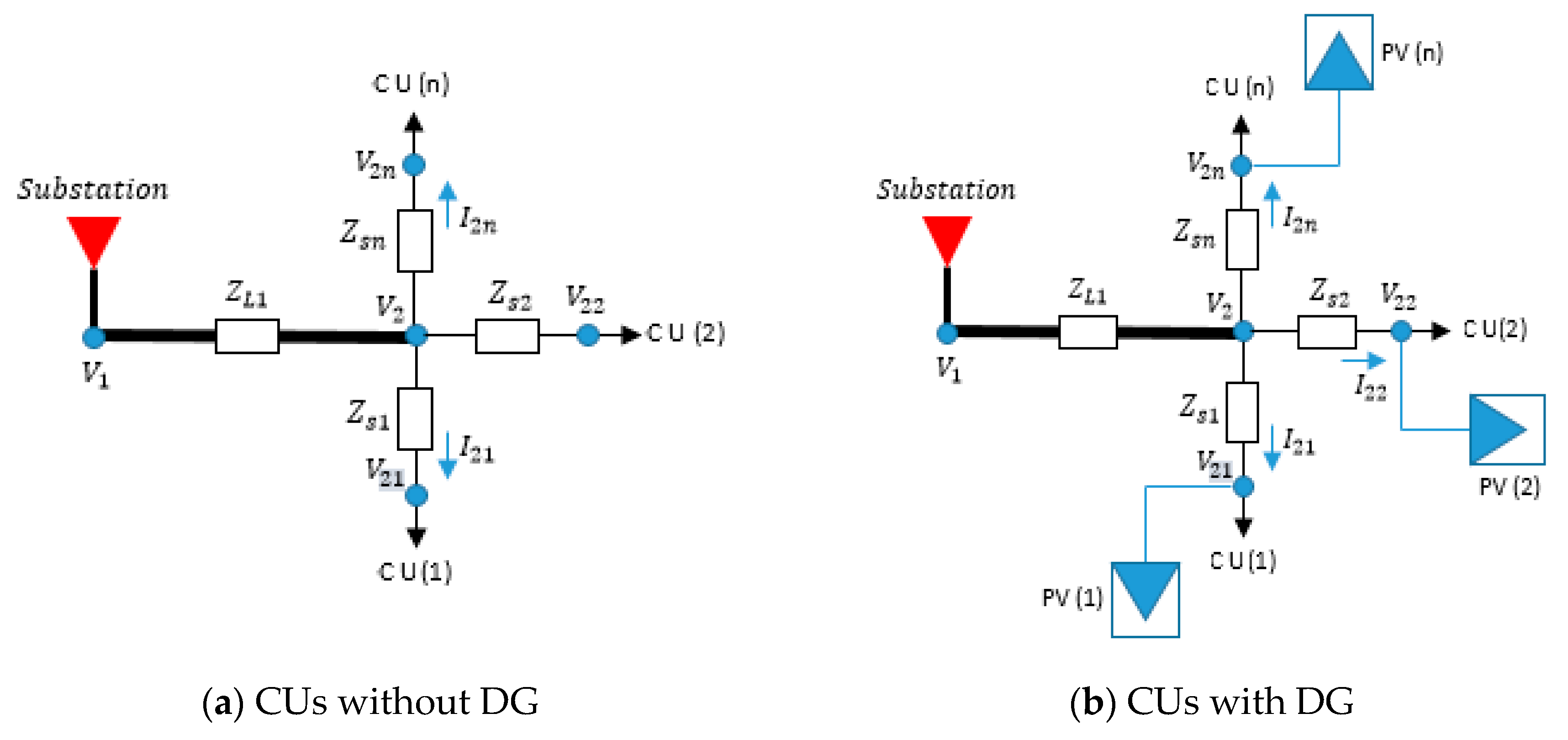
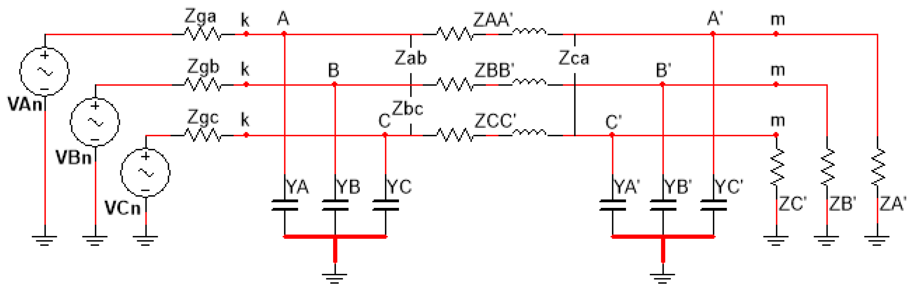
4.1. Network Electrical Parameters Modeling

The electrical representations of the transmission lines involve a series of factors and, in general, the study is performed in two configurations: Curved lines and long lines, being selected from the level of precision required by the study [19]. In this article, a long line model was chosen, generally used in large extension transmission lines, and is illustrated in Figure 6
Circuit interpretation in Figure 6 reveals there is a power transfer from the k bar to the m bar, through the TL (transmission line) with line impedance predominantly reactive. The presence of shunts elements and capacitors, are visualized in the extremities of the circuit, which are the result of the electric field effect between phase and guard conductors and the soil.
The mathematical representation of TL parameters is seen in Figure 6, and shown in Equation (4), separated in function of the resistive and reactive components of the network.
[ Z AA km Z AB km Z AC km Z BA km Z BB km Z AC km Z CA km Z BA km Z CC km ] = [ r AA km r AB km r AC km r BA km r BB km r AC km r CA km r BA km r CC km ] + j [ x AA km x AB km x AC km x BA km x BB km x AC km x CA km x BA km x CC km ]
Shunt capacitive impedance is tiny, and therefore is represented by its inverse, the susceptance. Shunt admittance is divided by half in each extremity and given by Equation (5).
Y shunt = j [ b AA km b AB km b AC km b BA km b BB km b AC km b CA km b BA km b CC km ]
In the feeder analyzed, as shown in Figure 3, the impedance of each network section is variable. This happens by economic strategy, because if the feeder were scaled with a uniform cross section throughout the circuit, it would imply high financial cost. For the purpose of modeling the electrical parameters of the feeder, the real impedance of each network section was considered, as well as the service extension that interconnects each CU to the circuit busbar.
Table 4 and Table 5 present the geometrical configuration of the feeder under study.
In Appendix A of this document are the impedance values considered in the network modeling, represented by the impedance matrix.

4.2. Photovoltaic System Modeling

The PVSystem element of OPENDSS is an energy converter, responsible for injecting active power to the bar, which in turn depends on solar irradiation, operating temperature of the photovoltaic panel, and inverter efficiency. Radatz [18] presented in his work the set of combined equations that result in the mathematical model used by the OPENDSS software to stimulate the electric power generated by a generator. Equation (6) estimates the power produced by the photovoltaic array, at each instant of time, using the Loadshapes presented in Figure 5 as a basis.
P ( t ) = Pmp base · I p . u . · I base · Pmp factor ( t )
Equation (6) calculates instantaneously the power produced by the PV panels, where Pmp base and I base are base quantities referring to the maximum power point of the generator and solar irradiance, respectively. I p . u . is the solar irradiance profile normalized by the reference radiation (1kWp/m2) throughout the day, shown previously in Figure 5. Power correction at the output of the PV’s is presented by the factor Pmp factor ( t ) .
The power effectively injected in the electrical network is given by Equation (7), also being expressed in function of time by the quantity Pca ( t ) .
Pca ( t ) = P ( t ) · ( η · P o )
The calculation of the power injected to the grid uses as basis the power produced by the PV panels, being dependent on the efficiency of the inverter to each load range. In this study, the photovoltaic generator modeling obeyed the conditions of a real system, where the electric companies establish a maximum power value for the connection of micro-generators to the grid, and such criteria are pre-established in [2].

4.3. Case Study

The main objective of this study was limited to a punctual analysis of section 8 of the feeder, which connects bar 08 to bar 09, and is responsible to supply six one-phase residential consumers and symmetrically distributed between the three phases available by the circuit of the feeder. Table 6 details all the configuration and layout of the CUs.
Upon technical requirements to access the power grid [2], a prosumer can produce its local electricity for self-consumption, being able to eventually export its energy surpluses for remote consumption. The combination of some factors as the conditions of solar irradiation, demand curve, and physical characteristics of service extensions can change the regular dynamic of the voltage profile, causing overvoltage at the point of delivery of the electric utility and unbalance in the three-phase network system. Currently, the inverters are equipped with protection systems that ensure system interruption (curtailment) given the occurrence of this phenomeno; in contrast, the unwanted shutdown of the photovoltaic system will imply in efficiency loss and more operational costs.
In order to identify these technical adversities in advance, in Figure 7 is shown a flowchart that performs a study of electrical voltage variability on permanent basis at the point of delivery of the CU, in function of the power installed of the photovoltaic DG. Simply put, the flowchart solves the load flow problem, returning with voltage values at the bars of the power grid and the CUs (Step 3); the values calculated are confronted with the established limits (Step 4); in case the values exceeds, the flowchart will return to Step 2 in order to reset the parameterization, restarting the load flow solution (Step 3). The algorithm is finished in the case of values remain at rated operating conditions (Step 5).
The problem is actually solved in the block that equates and analyzes the power flow, that is Step 3, identifying the potentials in the desired bars; with that, in Step 4, the voltage is verified according to the limits already mentioned in [14]. If the voltage limit is exceeded, it is necessary to make decisions that enable the insertion of photovoltaic generator safely to the PES (power electric system).
Simulation was performed through the OPENDSS-EPRI software, open source. The solution of the power flow is obtained through the interactive algorithm for the solution of load flow based on the Newton method. The input parameters for the simulation were obtained from a data acquisition system, which experimentally monitored the operating variables of the photovoltaic generator, the CU and the environmental conditions.
The simulation cases were selected from several combinations between input parameters. Next, the simulation combinations used to obtain the results are presented. The scenario represented by Figure 8 illustrates typical behavior of remote residential consumers, commonly idle during the entire day for a long monthly period, which can be compared to a sporadically inhabited rural property. The profile illustrated also represents single families CUs that are operationally idle during the day, usually having a nightly over-demand.
It is common that residential CUs do not support photovoltaic system, especially because there is no area for its installation (area occupation factor), but thanks to the power sharing mode, a photovoltaic system can integrate the local power system, being generated in another location (remotely). The demand curve above reaches a maximum of 190 W, in power terms, and equals a monthly average consumption of 78 kWh/month.
In addition to the load curve, the profile of solar irradiance for a clear sky day is represented in the same graph, as well as the operational temperature of the photovoltaic panel. The mismatch between the variables is very noticeable, and this is crucial in the results and consequences coming from simulation results.

5. Results

In the distribution feeder, it was delimited an interest zone. Figure 9 shows the gradual insertion of PV generators in the CUs. Bar 09 is located downstream from the substation (last bar), configuring a critical spot from an operational point of view. In this bar, six one-phase residential consumers are connected and distributed in the phase sequence already shown in Table 6.
In the simulation, the PV generation penetration was customized up to the maximum limit allowed in one-phase configuration, according to Table 2, and the DG was gradually inserted into each CU. The results were divided in two simulation cases, assuming the conditions imposed on [14] limiting the installed power for one-phase systems to a maximum 15 kW. The cases were partitioned into:
  • Case 1: P PV = 5   kW , 33% of maximum limit allowed.
  • Case 2: P PV = 10   kW , 66% of maximum limit allowed.

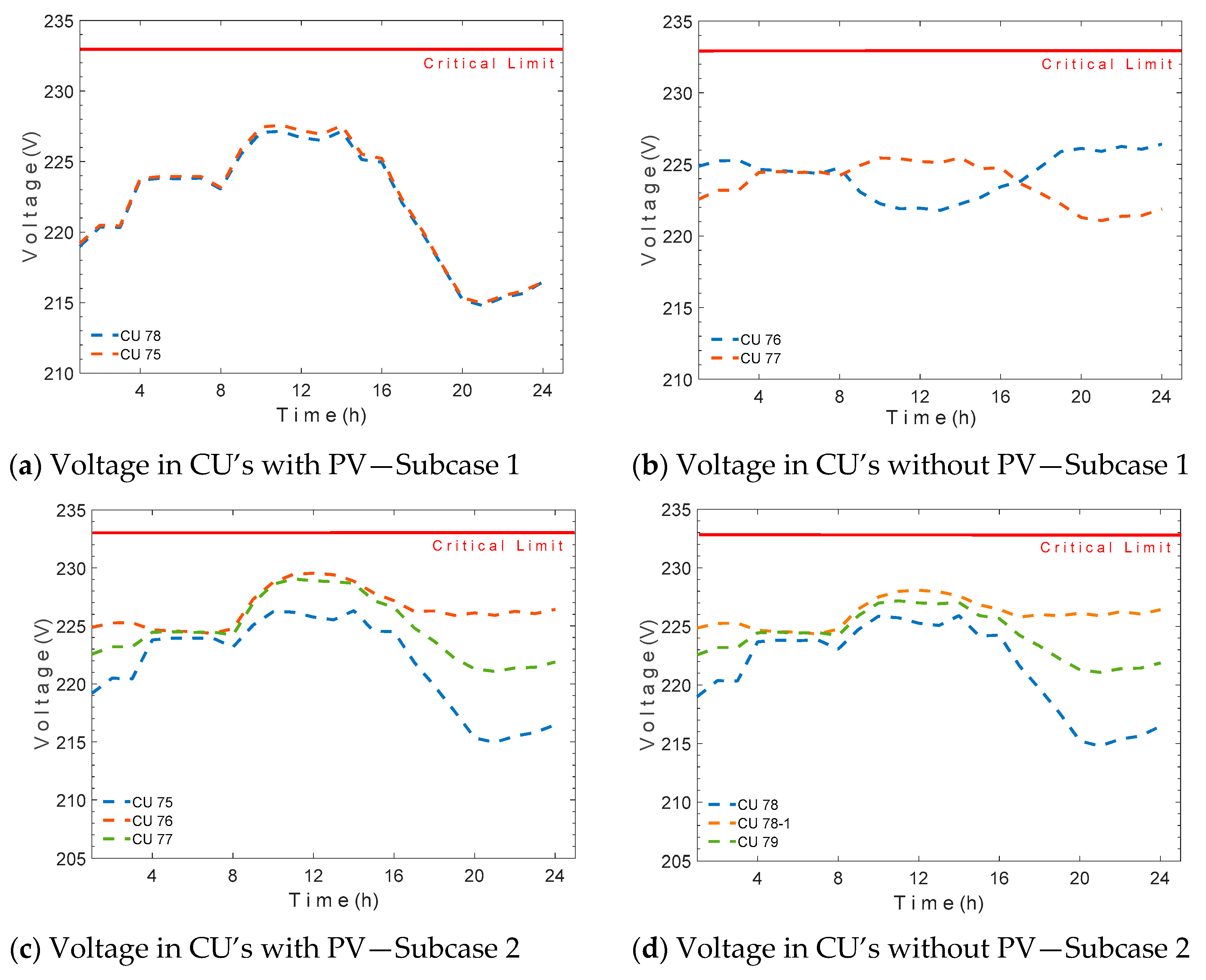
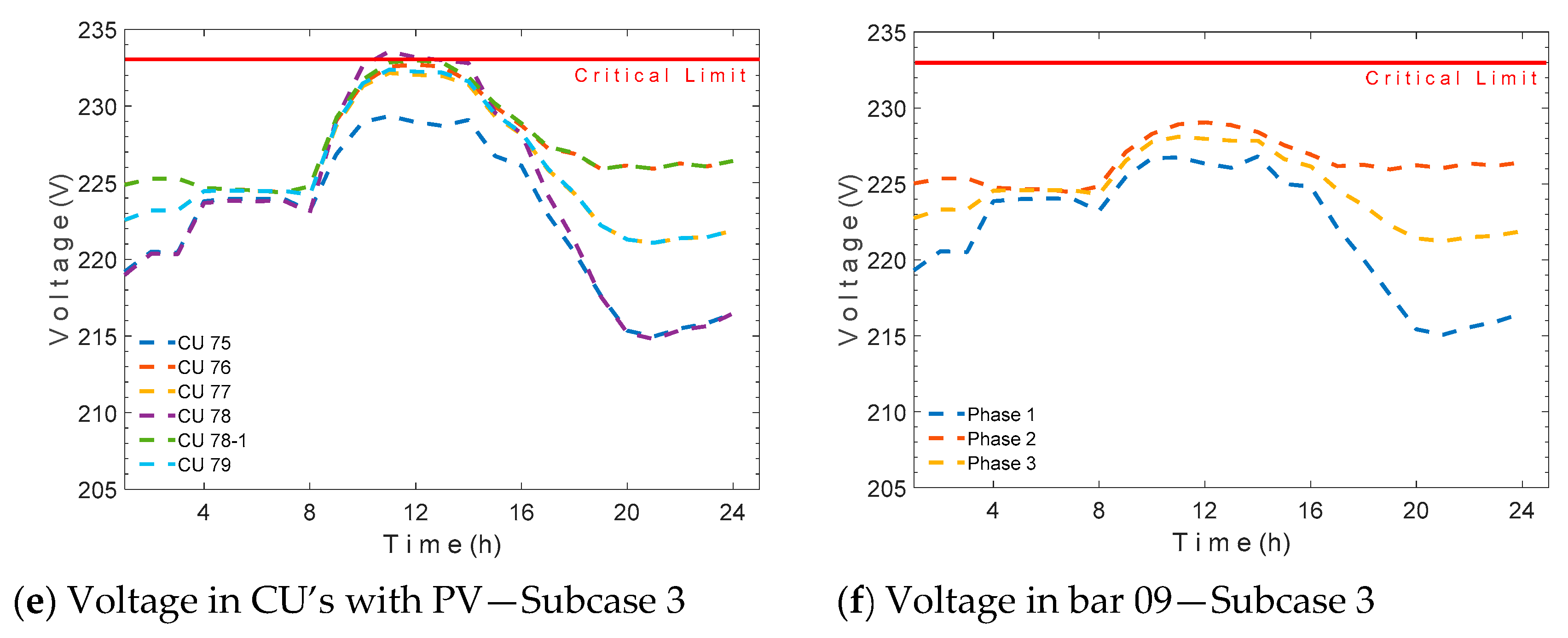
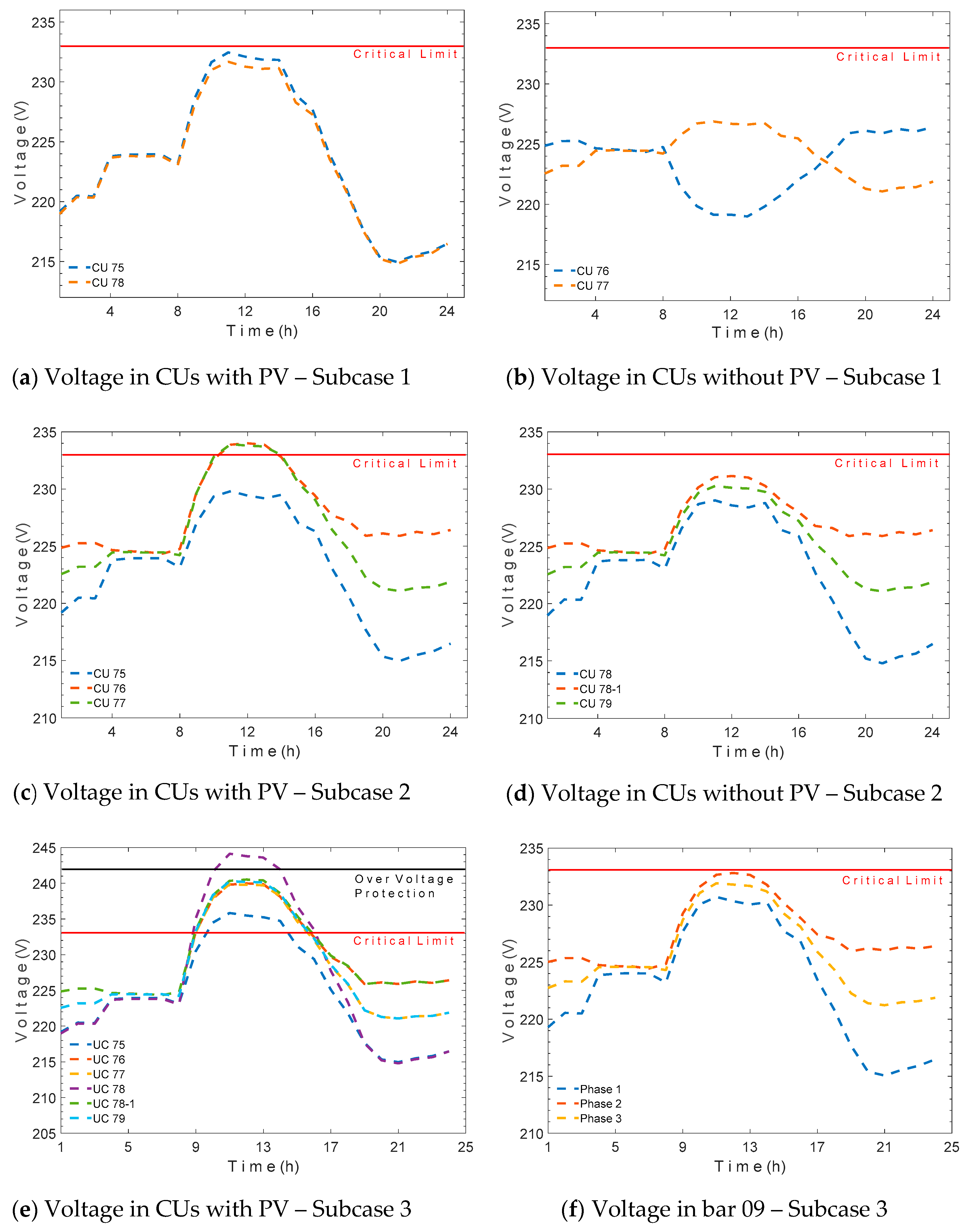
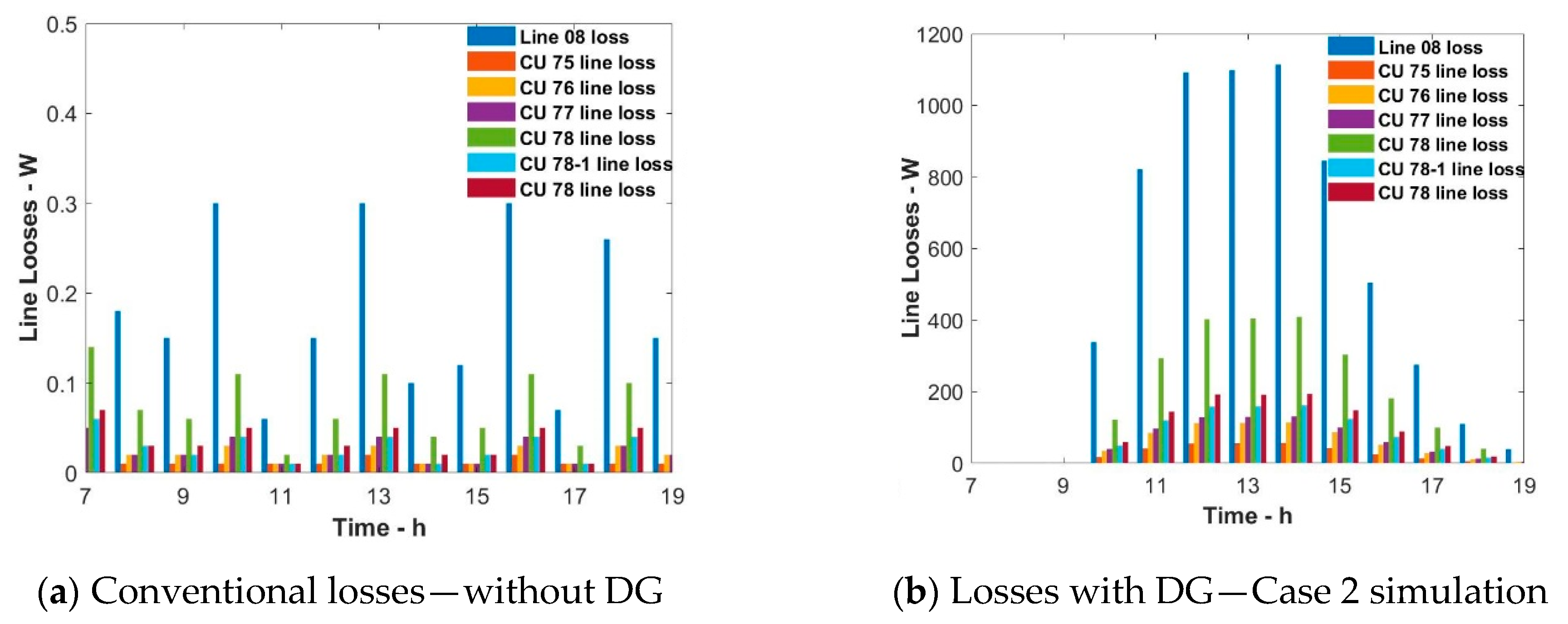
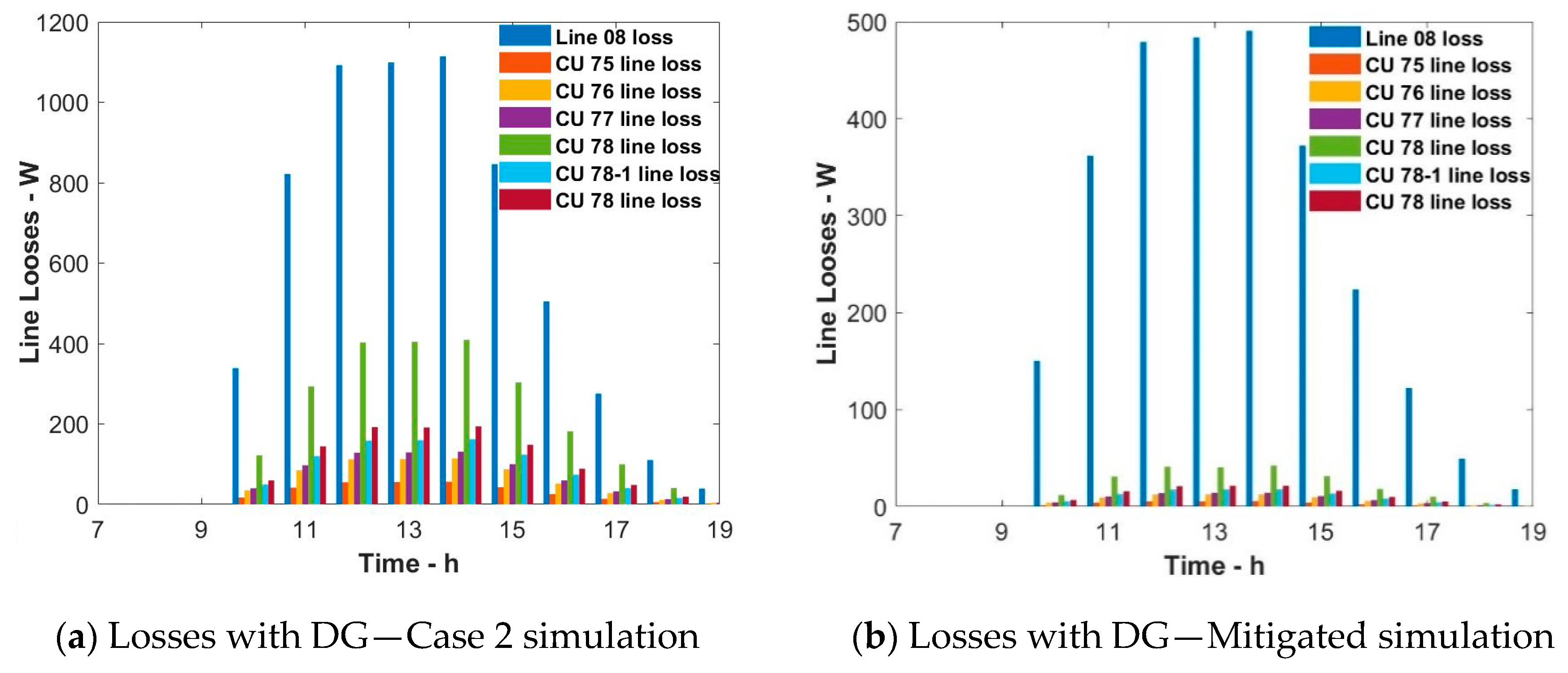
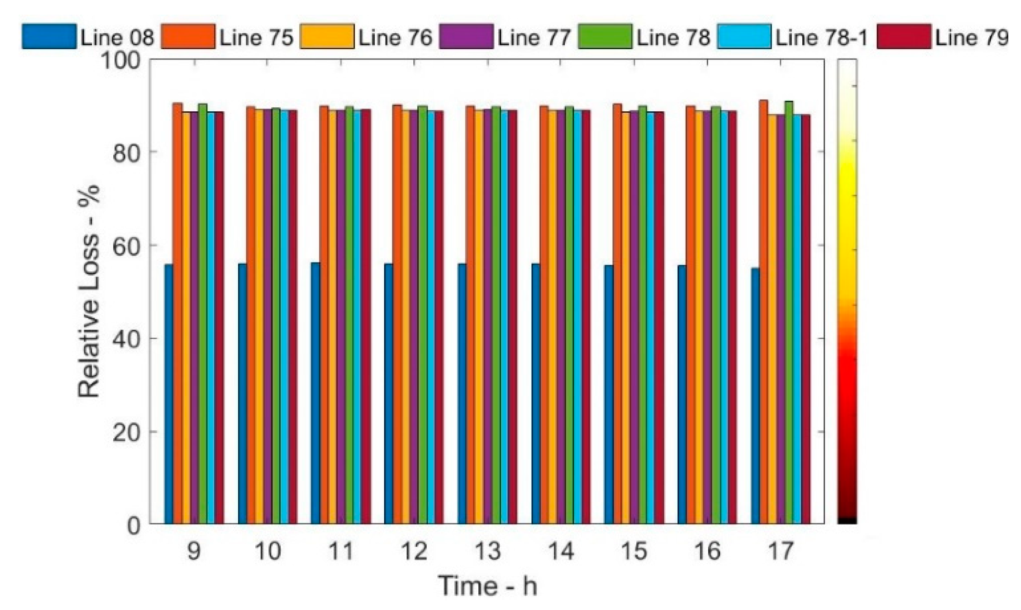
5.1. Simulation Results

Cases 1 and 2 were divided into three subcases that define the DG penetration criteria:
  • Subcase 1: Only one CU with PV;
  • Subcase 2: Three CU’s with PV;
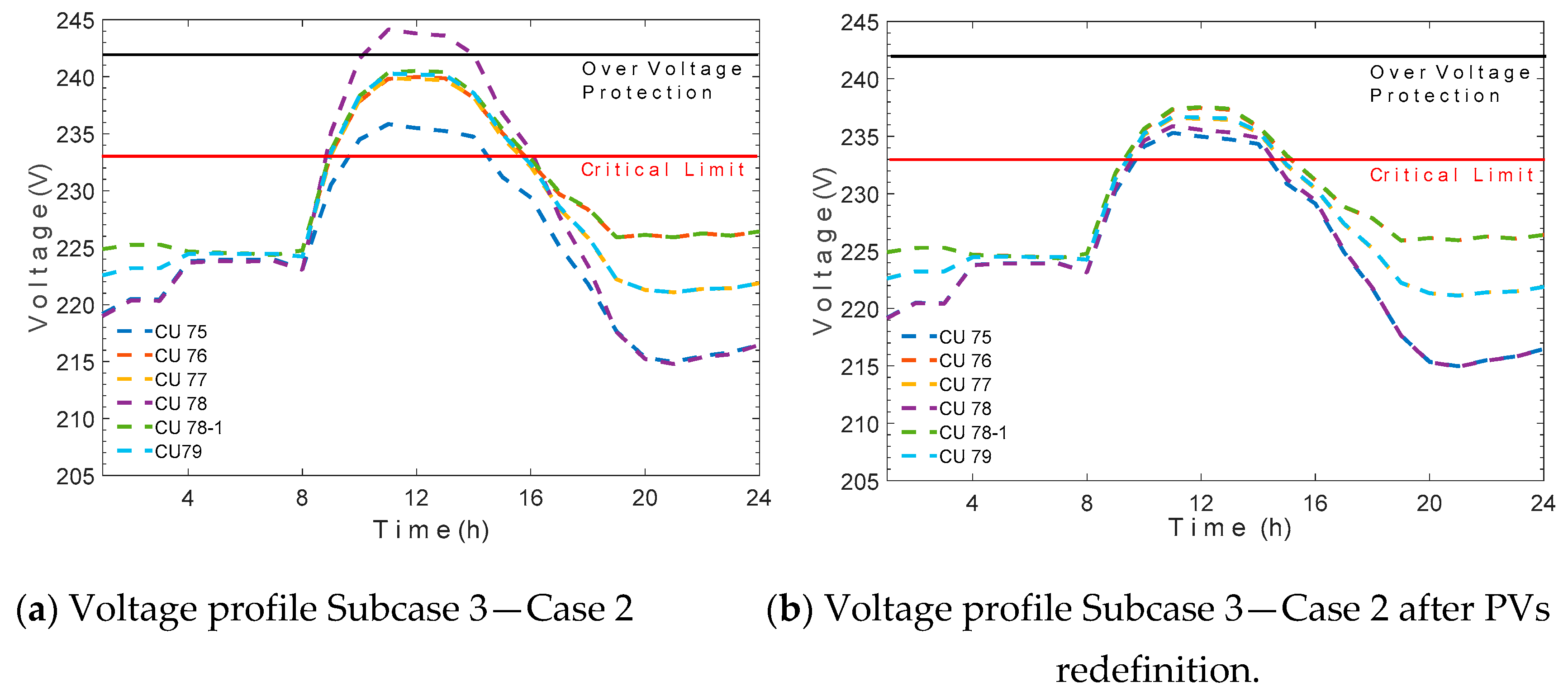
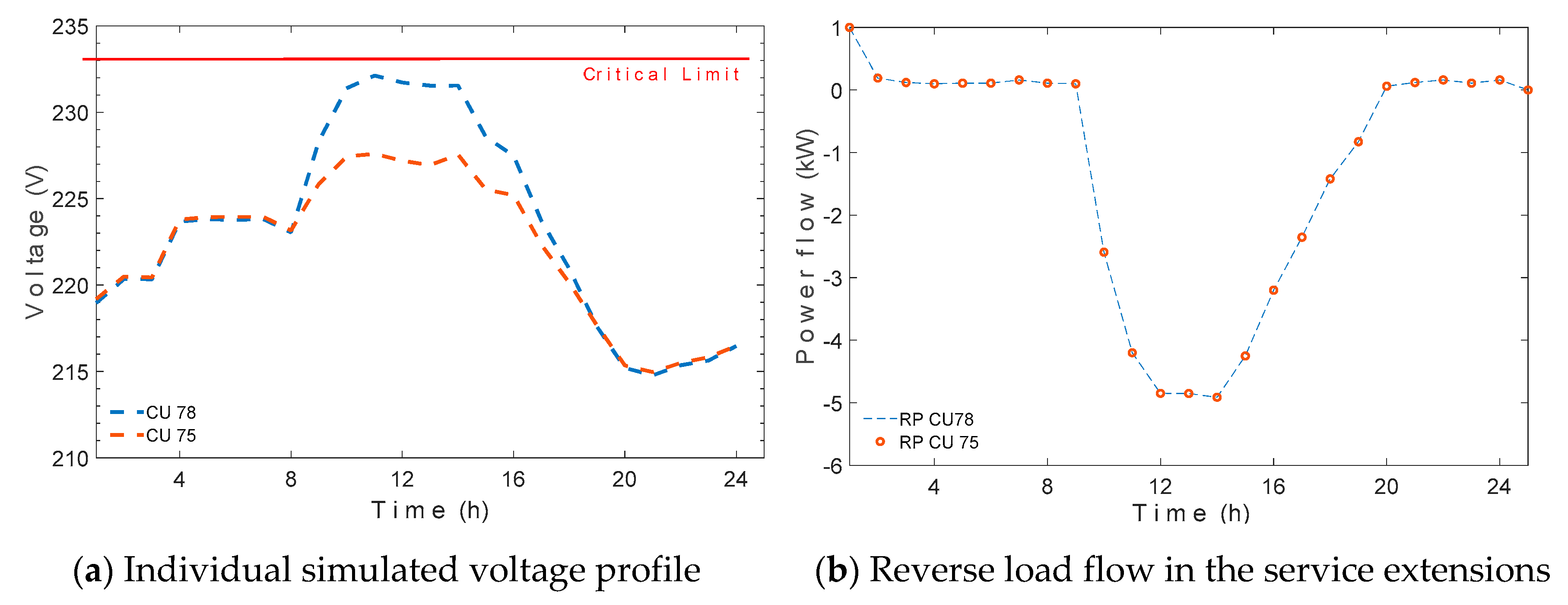
  • Subcase 3: All the CU’s with PV.
Case 1 simulation considered the gradual insertion of DG, keeping constant irradiance and demand conditions (according to Figure 8). The power installed for the photovoltaic generation units assumed in the subcases was fixed initially at 5.2 kWp. According to the three subtopics mentioned above, the levels of penetration for the subcases were 16%, 50%, and 100%, respectively. Subcase 3 corresponded to 41.6% of total power from the substation serving this extension, as well as subcase 1, that contemplated only 7% of total power from the substation. Table 7 below presents synthetically the methodological organization for simulation:
Cases 1 and 2 considered the installed power variations of photovoltaic generation; the subcases of photovoltaic penetration are incremented by the topics described in the first paragraph of this article and the power values of 5 kW and 10 kW correspond to cases 1 and 2, respectively.
The graphs in Figure 10 present the dynamic of voltage in the CUs connected to bar 09, for all subcases. Both graphs are limited by a red line expressing the maximum limit of electric voltage established [15].
On the graphs for subcases 1 and 2, it is noticed that the voltage levels are below the allowable limit. In subcase 1, only one PV generator connected to the electrical system was considered, corresponding to 34% of the allowed on one-phase topology. In this first moment, it is possible to see that CU 78 also suffers a minimal voltage increase, the effect arising from electricity generation from PVs connected to CU 75. The CUs interconnected to phases 2 and 3 tend to be more constant throughout the day, presenting a relative average dispersion for phase 1 of approximately 3%. Amplifying the number of PV generators to the electrical system, keeping constant the potency of the PVs (5 kW), a more symmetrical distribution of the voltage profile is noticed, varying only the amplitude of the voltage module, when comparing the CUs with and without PVs (Figure 10c,d).
In subcase 2, electrical voltage remained within the allowed limits and the CU 76 and 77 obtained overvoltage in relation to the other CUs, reaching 5% over CU 75, approaching critical value. This fact is due to the conductor employed in the service extension (Table 6), the variable related to the cross section and the length, which directly interfere with the electrical parameters. The last stage of case 1 analysis (subcase 3) takes into consideration all CUs equipped with PV generator, contemplating 100% penetration at bar 09. Observing Figure 10e, the reach of voltage maximum limit for CU 78 is confirmed, without surpassing it.
According to regional utility regulation [15], the service extension should be scaled to meet the maximum expected demand, and such fact is partially counterpointed in subcase 3 (Figure 10e). Still, in evidence for subcase 3, the three-phase voltage in bar 09 remains balanced and tolerated within the demanded values (shown in Figure 10f).
Simulation for case 2 also refers to items presented in Table 7, considering the installed PV potency of 10 kW, corresponding to 66% of maximum limit allowed on the network in one-phase configuration.
With all simulations performed for case 2, Even with the increase of the installed power of the DG, the voltage at the connection point remains acceptable, as seen in Figure 11a, other CUs without DG and connected to the same phase sequence are not influenced by overvoltage, the voltage profile may be seen in Figure 11b, the violation of the critical limit for CUs 76 and 77 can be seen in Figure 11c, although such variation is tiny and still ensures feeder security and operability. Voltage variation between phases of CUs in Figure 11c is on average between 1.7% and 1.9%. Still for subcase 2, CUs without DG remained with the voltage values within the required (Figure 11d) The situation is more critical in subcase 3 (Figure 11e), where practically all consumer units surpass voltage critical limit and the CU 78 reaches maximum voltage value, breaking the protection parameter against overvoltage of the inverter. CU 78 surpasses 5% of the critical voltage value, corresponding to 11% of nominal value. Below, the voltage relative variation percentage for critical and nominal limit, 233 and 220 volts, respectively, are shown.
Referring to subcase 3, where all CU’s are equipped with distributed generation of the same rated power installed and under the same demand length, the three-phase voltages seen from the mains side remained within the values required by normative resolution, as illustrated by graph of Figure 11f.
It is possible to verify the level of variability of the supply voltage of the CUs (Figure 12) around the critical limit (232 V) and the nominal value (220V), respectively shown by Figure 12a,b. The consumer unit 78 presented the highest amplitude in voltage increase, such effect was motived by the impedance of the service line and the installed power of DG.
Changes in penetration level of photovoltaic generator present large variations in the electrical system phases in CUs that are connected in the same phases, even with all residencies under the same demand and solar irradiation conditions, it is verified that unbalance level (∆U) occurs between CUs 75 and 78 with ∆U of 4%. The Table 8 below quantifies significantly the voltage variations between the CUs connected to the same phases and to distinct phases.
Subcase 3 presents higher rate of variation between consumers connected to phase V A . Fitted into the flowchart (Figure 7), the simulation will return to step 2 through the verifying routine (step 5). As a partially mitigating solution, the PVs were partitioned into three-phase configuration, where the power injected in the network by phase was reduced by 30% of PV nominal power. From these considerations, the simulation of load flow was particularly remade for subcase 3 and can be seen graphically below.
The mitigating solution adopted to reduce voltages in the CUs was the redefinition of the PVs connection, distributing all the power from the photovoltaic system simultaneously in three phases. The effect is verified in Figure 13; despite remaining above critical limit allowed, maximum overvoltage located in CU 78 were reduced in 4%. Table 9 below compares the phase asymmetry for both cases, showing the subcase 3 belonging to case studies 1 and 2, as well as the results of the mitigating effect. Cheol Jeong [20] related in his work a voltage control strategy that uses the step voltage regulator (SVR), one of the found results that after using the SVR it was possible to release a capacity of 2.7 MW more, maintaining the voltage levels specified. Shin [21] investigated the delivery voltage of the on-load tap-changers OLTC such that a large-capacity DG would not create unsafe voltage variations when penetrating the distribution network.
It is noticeable from the verification of the reduction of the voltage variation that when the PVs are redefined, the symmetrical distribution of the phases significantly improves the voltage quality in the three-phase circuit, allowing equilibrium. From a technical losses point of view, the impact in electrical losses reduction was noticed in the conductors belonging to the circuit of the power grid section and service extensions to consumer units. From the feeder’s operational profile, it is simple to conclude that electrical losses will be relatively low, although relevantly aggravated when there is too much increase in photovoltaic systems connected to the power grid. Figure 14 presents a comparison of technical losses evolution in the studied feeder, were Figure 14a considers the absence of distributed generation and Figure 14b considers the case of massive insertion of photovoltaic generators connected to a single phase
With the results shown in the graphs of Figure 14, the aggressive impact of distributed generation in electrical losses of the line each hour is evident. Please note that, at this moment, maximum penetration of photovoltaic systems in the bar under analysis is considered, all with nominal power of 10kWp. Comparing daily losses in the feeder section (section 08) for both cases, in the absence of DG, the losses in section 08 reached 5.11 Wh/day, and in the face of massive insertion, 6244 kWh/day was obtained, around 1200 times higher than normal condition.
The impact of technical losses is also seen when the load flow study is reconsidered in the simulation based on mitigation strategy adopted in this article, based on symmetrical distribution of nominal power of photovoltaic generator by phase. Figure 15 graphically illustrates the comparison between technical losses in the line for high concentration of photovoltaic systems connected to only one phase, and photovoltaic systems symmetrically distributed in the three-phase system.
Taking as reference the network section of the feeder (section 08), it is evident from the graphs above that the losses were severely reduced, around 55.78%. The mitigating strategy divides the installed power from a photovoltaic generator of 10 kWp located in a CU symmetrically in the three phases. For practical purposes, this is possible with the employment of a three-phase inverter or three one-phase micro-inverters, consequently relieving the conductors loading. In the service extensions to the CUs, there was also a reduction of losses, however the extension physical characteristics from each consumer unit vary according to the type of conductor, distance, and installation method, implying relatively different loss values. Losses reduction in the service extensions decreased 89.16%, obtained through an average of the extensions. The following graph (Figure 16) addresses the relative reduction of technical losses by extension against the massive insertion of photovoltaic generators, but strategically based on the mitigating solution.
Partitioning a photovoltaic generator unit from electrical losses reduction point of view is quite livable. It is possible to guarantee that the service extensions cooperate under normalized loading conditions, optimizing the load flow. On the other hand, the use of this configuration may not be as economically attractive, for conditioning the use of more devices. A solution to minimize losses can be seen in Gkaidatzis et al. [22] where the size and allocation of DG units was presented in order to minimize losses.

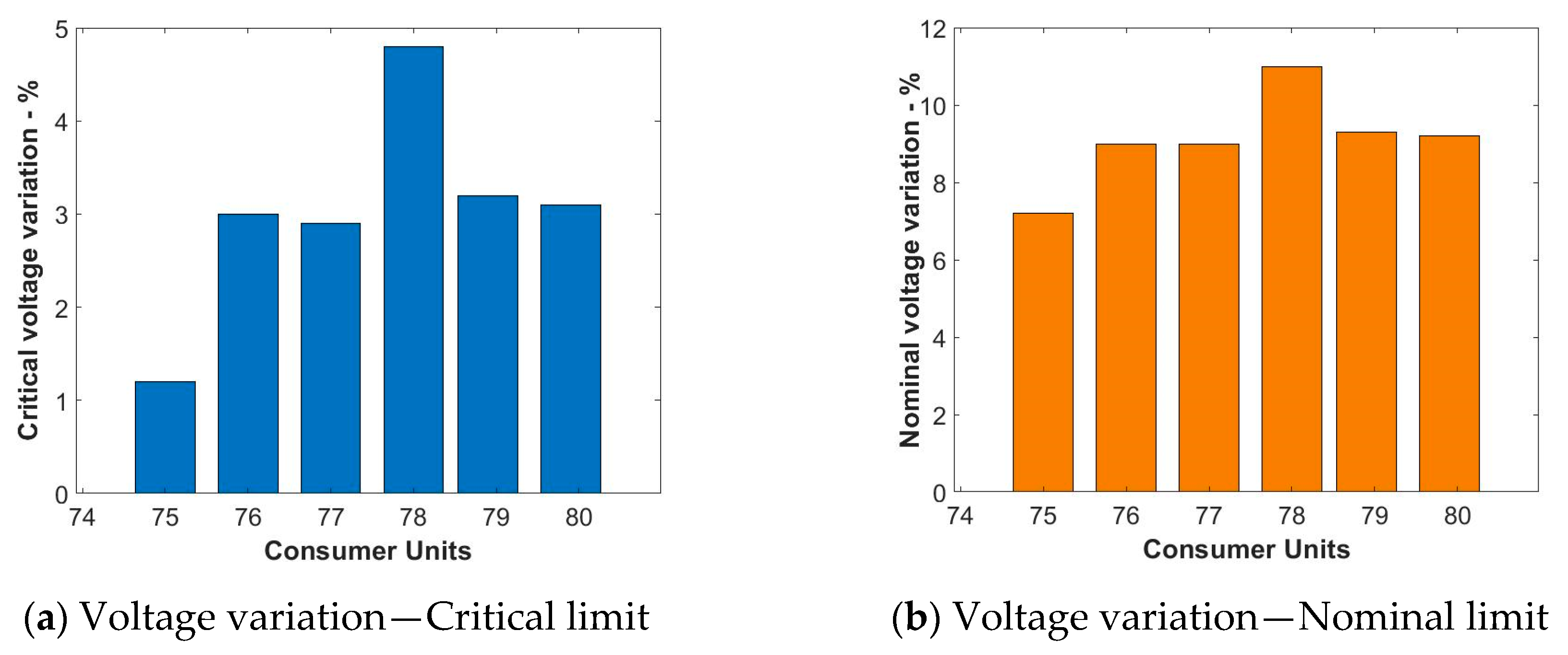
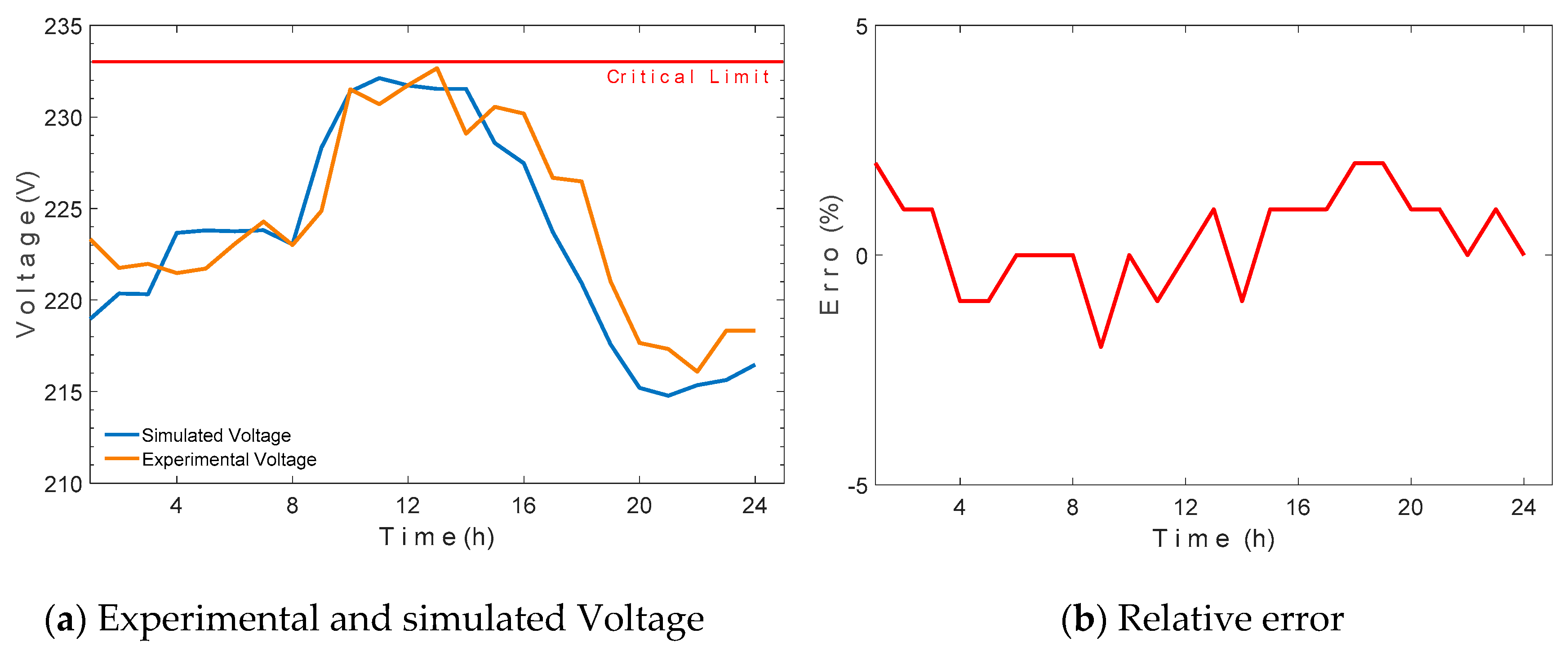
5.2. Experimental Data Result

An experimental array (CU) was developed in this case study to perform the comparison between the simulated and measured data. In the real context, the CU 78 was entirely instrumented storing and generating data used as input parameters in the simulations.
Several levels of massive insertion of systems in bar 09 were considered in the simulation. Subcase 1 analyzed initially was extracted to compare the dynamic of electrical voltage with real data extracted from CU 78. As shown in Figure 17a, the simulated voltage presents a similar behavior to experimental voltage.
The comparison performed between experimental and simulated voltages presented maximum relative error of ±2% (Figure 17b). The real voltage profile obtained from SCADA proves stability below maximum critical limit defined, corroborating with the simulation, and it is noticed that the interaction between the service extension from a CU and reverse power flow will result directly in the voltage behavior. The simulation performed initially in case 1, subcase 1 (Figure 10a) was repeated to verify the interference of the extension in the presence of reverse load flow. Therefore, a new PV was defined, this time connected to another CU (CU 78) and the simulation remade, keeping constant all premises from case 1, comparing with the previous result. The results can be seen in the graphs below.
Figure 18 portrays the influence of physical aspects and type of conductor employed in the service extension in the divergence that occurs in voltage values (Figure 18a). The larger amplitudes occur when the circuit is reverse loaded, in the period between 09:00 and 16:00, with the effect caused by the mismatch between the demand curve and electric generation. Figure 18b proves the constant behavior of the reverse power flow for both simulations and CUs, where the overvoltage in the simulation with CU 78 is 2% higher regarding the simulation in subcase 1, based on CU 75.

6. Conclusions

This article presents a load flow simulation in a secondary electrical power distribution feeder based on OPENDSS open-source tool. An analysis of the electrical voltage variable is performed, seen from the consumer when it is equipped with a photovoltaic electricity generation system. The electrical modeling of a power feeder was performed, as well as the allocation of the loads and the PV generators, matching the simulation scenario with the actual context. The simulation results proved that, in the occurrence of massive penetration of photovoltaic systems in one-phase connections with maximum power installed of 10 kWp, there was an overvoltage effect in the consumer units, countering the local regulations, which allows network connections of photovoltaic systems with one-phase configuration with up to 15 kWp. The solution for the overvoltage problem was mitigated by changing the connection type of PV systems to three-phase, ensuring voltage regulation within limits pre-established by normative resolution; it would also be possible to repower the service extension and keep the configuration. In the simulation considering partial insertion of PVs, voltage-raising effect spreads in CUs without DG but are connected to the same bar knot. Overvoltage results obtained in the experiment come from a combination of characteristics of service extension, local demand profile, and photovoltaic generator global characteristics, and it is possible to identify that the voltage tends to reach operating critical limit. Theoretical and experimental comparison is based on subcase 1 (considering only one DG insertion with 5 kWp of nominal power connected to the bar of the distribution system), where it is possible to verify a bias between voltage curves, ensuring the fidelity of the result. In general, this work proposes an analysis methodology based on a free software in the regulation restrictions to allow the access of new users to the low-voltage network in a way to ensure stable and incorrupt operation of the electrical system.

Author Contributions

I.C.T. developed all the theoretical study, contemplating the modeling and computer simulation, as well as all the writing of this paper. G.F.N. and C.T. have supervised and commented on this article.

Funding

This research received no external funding.

Acknowledgments

We thank the Conselho Nacional de Pesquisa (CNPq) Grant No. 302251-2017-0 and Universidade Federal de Pernambuco, for supporting the solar energy research projects and providing the material means and the scientific environment for the execution of this research.

Conflicts of Interest

The authors declare no conflict of interest.

Appendix A

In addition to this study, the representative impedance matrices of conductors that compose the distribution network were used. Equations (A1)–(A3) contemplate a series impedance of all network sections and are effectively used in the load flow calculation to determine the voltages and active losses on the line.
[ Z AA km Z AB km Z AC km Z BA km Z BB km Z AC km Z CA km Z BA km Z CC km ] = [ 1.145 0 0 0.55 1.145 0 0.55 0.55 1.145 ] + j [ 0.9415   0 0 0.8288 0.9415   0 0.8288 0.8288 0.9415 ]
[ Z AA km Z AB km Z AC km Z BA km Z BB km Z AC km Z CA km Z BA km Z CC km ] = [ 1.342033   0 0 0.5467333 1.342033 0 0.5467333 0.5467333 1.342033 ] + j [ 0.9546 0 0 0.8418 0.9546 0 0.8418 0.8418 0.9546 ]
[ Z AA km Z AB km Z AC km Z BA km Z BB km Z AC km Z CA km Z BA km Z CC km ] = [ 1.755767 0 0 0.4666667 1.755767 0 0.4666667 0.4666667 1.755767 ] + j [ 0.9692 0 0 0.85 0.9692 0 0.85 0.85 0.9692 ]
The simulated system contains 20 bars, base voltages of 0.38 kV and 0.22 kV and base power of 100 MVA were adopted. For CUs parameterization low loading residential curves were used, experimentally raised with PF = 0.98.

References

  1. IEA. Renewable Energy. In Medium-Term Market Report 2016; IEA Publication: Paris, France, 2016; pp. 1–282. [Google Scholar]
  2. ANEEL. Resolução Normativa nº 687, de 24 de Novembro de 2015; Agência Nacional de Energia Elétrica: Brasilia, Brazil, 2015.
  3. Negreiros, F.G. Impacto da Instalação Massiva de Sistemas FV Distribuídos no Desempenho da rede Elétrica. Master’s Thesis, Universidade Federal de Pernambuco, Recife, Pernambuco, Brasil, 2018. [Google Scholar]
  4. Chen, B.; Sun, P.; Liu, C.; Chen, C.L.; Lai, J.S.; Yu, W. High Efficiency Transformerless Photovoltaic Inverter with Wide-range Power Factor Capability. In Proceedings of the Applied Power Electronics Conference and Exposition (APEC), Orlando, FL, USA, 5–9 February 2012; pp. 575–582. [Google Scholar]
  5. Análise de Operação de Sistemas de Distribuição Utilizando o OpenDss. Available online: https://docplayer.com.br/80921193-Analise-de-operacao-de-sistemas-de-distribuicao-utilizando-o-opendss.html (accessed on 27 October 2019).
  6. Chathurangi, D.; Jayatunga, U.; Rathnayake, M.; Wickramasinghe, A.; Agalgaonkar, A.; Perera, S. Potential Power Quality Impacts on LV Distribution Networks with High Penetration Levels of Solar PV. In Proceedings of the 18th International Conference on Harmonics and Quality of Power (ICHQP), Ljubljana, Slovenia, 13–16 May 2018. [Google Scholar]
  7. Reno, M.J.; Coogan, K.; Broderick, R.J.; Grijalva, S. Reduction of Distribution Feeders for Simplified PV Impact Studies. In Proceedings of the IEEE Photovoltaic Specialists Conference, Tampa, FL, USA, 16–21 June 2013. [Google Scholar]
  8. Chiconi, D.N. Monitoramento e Análise da Geração Distribuída em Sistemas de Distribuição de Energia Elétrica. Trabalho de conclusão de curso, São Carlos, São Paulo, Brazil. 2017. [Google Scholar]
  9. De Carne, G.; Buticchi, G.; Zou, X.Z.; Liserre, M. Reverse power flow control in a ST-fed distribution grid. IEEE Trans. Smart Grid 2018, 9, 3811–3819. [Google Scholar] [CrossRef]
  10. IEA-PVPS Task 14—High Penetration of PV Systems in Electricity Grids Work-Plan 2010–2014. Available online: https://anaiscbens.emnuvens.com.br/cbens/article/view/177 (accessed on 27 October 2019).
  11. Sayeef, S.; Moore, T.; Percy, S.; Cornforth, D.; Ward, J.; Rowe, D. Characterization and Integration of High Penetration Solar Power in Australia: A Solar Intermittency Study. In Proceedings of the 1st International Workshop on the Integration of Solar Power into Power Systems, Aarhus, Denmark, 24 October 2011. [Google Scholar]
  12. Procedimentos de Distribuição de Energia Elétrica no Sistema Elétrico Nacional—PRODIST, Módulo 8—Qualidade da Energia Elétrica. v. 9. Available online: https://www.aneel.gov.br/prodist (accessed on 27 October 2019).
  13. Xie, Q.; Shentu, X.; Wu, X.; Ding, Y.; Hua, Y.; Cui, J. Coordinated Voltage Regulation by On-Load Tap Changer Operation and Demand Response Based on Voltage Ranking Search Algorithm. Energies 2019, 12, 1902. [Google Scholar] [CrossRef]
  14. Procedimentos de Distribuição de Energia Elétrica no Sistema Elétrico Nacional—Prodist, Módulo 3—Acesso ao Sistema de Distribuição Revisão. v. 7. Available online: https://www.aneel.gov.br/prodist (accessed on 27 October 2019).
  15. ED-AL. Norma Técnica para a Conexão de Acessantes a Rede de Distribuição das Distribuidoras da Eletrobrás—Conexão em Baixa Tensão; Eletrobras Distribuição Alagoas: Maceió, Brazil, 2013. [Google Scholar]
  16. ED-AL. Manual de Procedimentos de Redes de Distribuição; Eletrobras Distribuição Alagoas: Maceió, Brazil, 2012. [Google Scholar]
  17. Beránek, V.; Olšan, T.; Libra, M.; Poulek, V.; Sedláček, J.; Dang, M.Q.; Tyukhov, I.I. New Monitoring System for Photovoltaic Power Plants Management. Energies 2018, 11, 2495. [Google Scholar] [CrossRef]
  18. Radatz, P.R. Modelos Avançados de Análise de Redes Elétricas Inteligentes Utilizando o Software OpenDss; Trabalho de conclusão de curso; Universidade de São Paulo: São Paulo, Brazil, 2015. [Google Scholar]
  19. Monticelli, A.; Garcia, A. Introdução a Sistemas de Energia Elétrica; Editora UNICAMP: São Paulo, Brazil, 2003. [Google Scholar]
  20. Jeong, C.; Lee, B.; Alleman, D. Reducing voltage volatility with step voltage regulators: A life-cycle cost analysis of Korean solar photovoltaic distributed generation. Energies 2019, 12, 652. [Google Scholar] [CrossRef]
  21. Shin, K.H. A Study on the Method for Controlling Sending-End Voltage for Voltage Regulation at the Distribution System with Large Distributed Generation. Master’s Thesis, Soongsil University, Seoul, Korea, 2015. [Google Scholar]
  22. Gkaidatzis, P.A.; Doukas, D.I.; Bouhouras, A.S.; Sgouras, K.I.; Labridis, D.P. Impact of penetration schemes to optimal DG placement for loss minimisation. Int. J. Sustain. Energy 2017, 36, 473–488. [Google Scholar] [CrossRef]
Figure 1. Simplified representation of an electrical distribution network.
Energies 12 04568 g001
Figure 2. Overvoltage in a service extension due to the excess of reverse power flow.
Energies 12 04568 g002
Figure 3. Single line representation of the feeder under study.
Energies 12 04568 g003
Figure 4. Representation of the simulation experimental environment.
Energies 12 04568 g004
Figure 5. Loadshapes used as input data in the power flow modeling.
Energies 12 04568 g005
Figure 6. Three-wire representation of a three-phase network.
Energies 12 04568 g006
Figure 7. Flowchart to determine the permissive index for photovoltaic systems.
Energies 12 04568 g007
Figure 8. Graphic profile of input parameters.
Energies 12 04568 g008
Figure 9. Study zone.
Energies 12 04568 g009
Figure 10. Simulated voltage dynamic profile for case 1.
Energies 12 04568 g010aEnergies 12 04568 g010b
Figure 11. Simulated voltage profile in case 2.
Energies 12 04568 g011
Figure 12. Representation of voltage variation around the reference values.
Energies 12 04568 g012
Figure 13. Voltage profile comparison in CUs before and after mitigation in subcase 3.
Energies 12 04568 g013
Figure 14. Electrical losses in feeder circuit.
Energies 12 04568 g014
Figure 15. Comparison of electrical losses in the feeder circuit.
Energies 12 04568 g015
Figure 16. Losses reduction with massive insertion of photovoltaic (PV) systems under mitigation effect.
Energies 12 04568 g016
Figure 17. Comparison of real and experimental voltage.
Energies 12 04568 g017
Figure 18. Individual simulation comparison of subcase 1 (case 1) for different consumer units (CUs).
Energies 12 04568 g018
Table 1. Voltage variation values in function of service voltage.
Voltage QualityRange 220 (Volts)
Normal202 ≤ V ≤ 231
Precarious191 ≤ V <202
231 < V ≤ 233
CriticalV < 191 or V > 233
Table 2. Service voltage in function of local demand.
ConnectionInstalled PowerVoltage
One-phaseP ≤ 15 kW220 V
Three-phase15 ≤ P ≤ 75 kW 380 V
Table 3. Definition of the bars for the power flow study.
Bar TypesInputOutputBarReal Feeder
PQ P k   and   Q k V k   and   θ k LoadB3 to B20
REFERENCE V k   and   θ k P k   and   Q k ReferenceB2
Table 4. Quantitative bars in the electricity distribution system.
SectionKnot 1Knot 2Length (km)SectionKnot 1Knot 2Length (km)
1B2B30.01711B12B130.024
2B3B40.01212B10B140.024
3B4B50.01313B2B200.017
4B5B60.01814B20B190.017
5B6B70.01115B19B180.022
6B7B80.02016B18B170.022
7B8B90.01817B17B160.005
8B4B100.03418B16B150.012
9B10B110.04019B15B140.005
10B11B120.012----
Table 5. Conductor specification by network section.
SectionConductorReferenceSectionConductorReference
1Al 70 mm2Trunk11Network endAl 25 mm2
2Al 70 mm2Trunk12Network endAl 25 mm2
3Al 70 mm2Trunk13Network endAl 25 mm2
4Al 50 mm2Derivation14NeutralAl 50 mm2
5Al 25 mm2Trunk15Network endAl 25 mm2
6Al 25 mm2Trunk16Network endAl 25 mm2
7Al 25 mm2Network end17TrunkAl 50 mm2
8Al 25 mm2Network end18TrunkAl 50 mm2
9Al 50 mm2Derivation19TrunkAl 70 mm2
10Al 25 mm2Trunk20TrunkAl 70 mm2
Table 6. Parameters of services extensions of bar 09.
LoadsPhaseVoltageExtension and Gauge Service Line
75A-N220 V2 m–04 mm2
76B-N220 V7 m–06 mm2
77C-N220 V9 m–06 mm2
78A-N220 V17 m–06 mm2
78_1B-N220 V10 m–06 mm2
79C-N220 V12 m–06 mm2
Table 7. Simulation subcases for cases 1 and 2.
CUSubcases 1, 2 and 3 of PV PenetrationCases (P = 5.0 kW and P = 10 kW)
755 kW–10 kW5 kW–10 kW5 kW–10 kW1–2
76-5 kW–10 kW5 kW–10 kW1–2
77-5 kW–10 kW5 kW–10 kW1–2
78--5 kW–10 kW1–2
78_1--5 kW–10 kW1–2
79--5 kW–10 kW1–2
Table 8. Simulation subcases for cases 1 and 2.
CasesSubcasesMaximum Voltage Drop Phases–VoltsPhase variation (∆U)
Distinct Phases
Phase variation (∆U)
Same Phases
V A V B V C V A B V B C V A C V A V B V C
1
P P V = 5 KW
1227.5226.4225.40.5%0.4%0.9%0.2%0.0%0.0%
2226.3229.5229.01.4%0.2%1.2%0.2%0.6%0.8%
3233.5232.9232.30.2%0.3%0.5%2%0.1%0.1%
2
P P V = 10 KW
1232.4226.4226.82.6%0.2%2.4%0.3%0.0%0.6%
2229.8234.0233.91.8%0.0%1.8%0.3%1.2%1.1%
3244240.5240.21.5%0.1%1.6%4%0.2%0.2%
Table 9. Simulation subcases for case 2.
SubcasesMaximum Voltage Drop
Phases–Volts (V)
Phase Variation (∆U)
Distinct Phases (%)
Phase Variation (∆U)
Same Phases (%)
V A V B V C V A B V B C V A C V A V B V C
3244.0 V240.5 V240.2 V1.5%0.1%1.6%4%0.2%0.2%
Mitigation235.8 V237.5 V236.7 V0.7%0.3%0.4%0.3%0.0%0.0%

