An Orderly Power Utilization Scheme Based on an Intelligent Multi-Agent Apanage Management System

Abstract

Orderly power utilization (OPU) is an important measure to alleviate contradiction between supply and demand in a power system peak load period. As a load management system becomes smarter, it is necessary to fully explore the interactive ability among users and make schemes for OPU more applicable. Therefore, an intelligent multi-agent apanage management system that includes a mutual aid mechanism (MAM) is proposed. In the decision-making scheme, users’ participation patterns and the potential of peak shifting and willingness are considered, as well as the interests of both power consumers and power grid are comprehensively considered. For residential users, the charging time for their electric vehicles (EVs) is managed to consume the locally distributed power generation. To fully exploit user response potential, the algorithm for improved clustering by fast search and find of density peaks (I-CFSFDP), i.e., clusters the power load curve, is proposed. To conduct electrical mutual aid among users and adjust the schemes reasonably, a multi-objective optimization model (M2OM) is established based on the cluster load curves. The objectives include the OPU control cost, the user’s electricity cost, and the consumption of distributed photovoltaic (PV). Our results of a case study show that the above method is effective and economical for improving interactive ability among users. Agents can coordinate their apanage power resources optimally. Experiments and examples verify the practicability and effectiveness of the improved algorithm proposed in this study.

1. Introduction

The smart grid plays an important role in improving the efficiency and quality of power supply. The peak clipping mode is widely used by power companies [1], but there are problems, such as severe peak power consumption and power shortage [2]. These problems can be solved by demand-side management (DSM), which mitigates power imbalance during peak load. The orderly power utilization (OPU) with the characteristic of “interaction” becomes the latest development direction of DSM [3].

DSM can improve patterns and efficiency of power consumption by stimulating demand-side resources (DSR) [4]. DSR includes electric vehicles (EVs), air conditioners, factories and companies, and other public places. The battery of an EV has energy storage characteristics that make it different from the conventional power load [5]. In the background of peak and valley electricity price, an effective guidance scheme can be developed through the load forecasting mechanism to make the EV respond to the discharge mechanism during the power consumption peak hours of daytime, and evenly transfer the charging load during the low valley at night [6]. For residential users, it adjusts the charging period of EVs to promote local consumption of distributed power.

In recent years, OPU has become an important part in a smart grid, and user initiative has becomer more obvious [7]. To ensure the effectiveness of the schemes, we have higher requirements for the management mode of OPU. Traditional non-OPU schemes rarely consider user willingness and patterns of participation [8]. Therefore, the obtained schemes are unreasonable and different from the actual situation, resulting in a waste of energy and investment [9]. To improve the accuracy of schemes, the participation patterns, willingness of users, as well as the interests of both the power grid and users should be fully considered. However, the users’ electricity consumption behavior is randomn and uncertain, and therefore the multidimensional data, caused by uncertainty, makes calculations difficult. Usually, the uncertainties in the planning process are simulated with random variables, using chance-constrained programming [10]. Another approach is a clustering algorithm [11,12], however, when there are many uncertainties, it is difficult to analyze mass data and improve computational efficiency. Therefore, it is important to reduce redundant data while ensuring the accuracy of the model.

Clustering technology can reasonably transform the uncertain model into a deterministic model. Traditional clustering algorithms include partition-based, hierarchy-based and density-based clustering algorithms. Partition-based algorithms run fast, such as k-means, but the theory of the initial clustering center and cluster number is not perfect [13]. The hierarchical algorithm has high space-time complexity and cannot be used in large data environments [14]. The density-based algorithm has prolonged data processing and it is hard to determine the key parameters [15]. In the case of large cluster shape differences and high data dimensions, the clustering effect, stability and clustering speed of current methods are unsatisfactory [16]. Therefore, it is urgent to establish a more effective clustering method.

To improve the accuracy and practicability of load curve clustering, we propose the improved clustering by fast search and find of density peaks (I-CFSFDP) algorithm. The clustering by fast search and find of density peaks (CFSFDP) algorithm can find clusters of arbitrary shapes and automatically determine the number of clusters [17]. The algorithm can quickly cluster high-dimensional mass data, and the clustering result is stable and effective [18]. Combined with the characteristics of high-dimensional mass and large cluster size of power load curve, the algorithm is improved. The algorithm refers to the idea of k-nearest neighbors (KNN) to make the algorithm more adaptive. I-CFSFDP can effectively reduce computational difficulties.

In the process of executing the OPU scheme, temporary adjustments sometime occur. If the user is not given the right to negotiate mutual aid, the user does not have enough time to cope with the unexpected situation and reduce the satisfaction of power consumption [19], which leads to inefficient execution and communication congestion [20]. Meanwhile, the fairness of the scheme needs to be improved. The intelligent multi-agent system (IMAS) is the main part in the field of distributed artificial intelligence [21]. The IMAS coordinates a group of intelligent agents with decentralized information and, then, negotiates to solve the problem in a short period of time [22]. This system is widely used in many fields of a power system, such as power system dispatch and topology analysis [23,24].

In comparison to the traditional OPU method, this study develops a personalized power consumption scheme based on user’s participation willingness [22]. We discuss the architecture of IMAS including using a mutual aid mechanism, MAM, which includes a multilayer power grid. The physical structure of the grid is divided into three layers, i.e., system, node, and user (system-node-user), and the index allocation mechanism from top to bottom is formulated. Considering the uncertainty, we argue that clustering technology can reasonably transform the uncertain model into a deterministic model, and effectively reduce the difficulty of modeling and solving. The uncertainty model can fully consider the time series. The I-CFSFDP method causes less damage to data characteristics and can accurately describe the data changes of the original scene. On the basis of the the load characteristic curve obtained by the I-CFSFDP, a multi-objective model is established. It considers the participation patterns, willingness of users, as well as the interests of both the power grid and users. The goal of the model is to minimize the total cost of both OPU control and users’ electricity consumption and maximize the local consumption of the distributed photovoltaic (PV). The forbearing stratified sequencing (FSS) method is used to solve the model [25]. We fully consider the user’s willingness, participation patterns and user’s interests as compared with other decision-making methods. The focus is on the user’s active features. Through a large number of comparative analysis, we show that the IMAS’s OPU scheme can reduce peak power consumption, improve execution efficiency, and fully exploit the potential of user interaction.

Considering the above issues, we proposes an IMAS with a MAM for OPU in a multilayer power grid. The major contributions are summarized as follows:

(1)

The initiative IMAS can achieve coordinated optimization within the jurisdiction, make decisions and adjustments to the power usage plan, and improve the efficiency of information transmission;

(2)

The proposed MAM can participate in the adjustment of the OPU plan, realize the mutual coordination between users, improve the user’s interactive ability and establish a aid order table to ensure the fairness of electricity consumption;

(3)

The proposed I-CFSFDP algorithm can effectively reduce the difficulty of modeling and solving, and can fully consider its time based on uncertain modeling of electricity consumption behavior;

(4)

The established multi-objective OPU decision model comprehensively considers the interests of both users and the grid, users’ willingness and taps the potential of users. FSS is used to solve the proposed model. It is verified by the load data from the Open Energy Information (Open EI) website of the U.S. Department of Energy [26]. The results show that the model is reasonable and the algorithm is effective. Definition of nomenclature are showed in

Table 1. Definition of nomenclature.

Nomenclature
$d_{ij}$	distance between sample i and j (Euclidean distance)	${\xi }^{clip}$	control cost coefficient of peak clipping
$d_c$	truncation distance	$M_{i,k}$	peak clipping grade
$\tau$	whole data set	${\eta }_{DG}$	PV conversion rate
$Q_i$	recipient capacity	$S_{DG}$	contact area of the battery plate
$W_i$	historical aid score.	$K_{DG}$	light radiation intensity
$Q_i=\left[Q_1,Q_2\dots Q_m\right]$	recipient capacity matrix	$n_{DG}$	number of the battery plates
m	number of recipient users	${\theta }_{out}^t$	external environment temperature.
$S_i=\left[S_1,S_2\dots S_n\right]$	aid capacity matrix	$P_{EV}\left(t\right)$	charging power of the EV in t-period
n	number of aid users	$P_{EV}$	rated charging power
${\rho }_i$	local density of each sample	${\mathrm{S}}_{EV}\left(\mathrm{t}\right)$	charging state, and 1 means charging
$\mathsf{\delta }$	local distance of each sample	$Q_t$	charging state of the battery in t-period
KNN (i)	KNN sample set of sample i	$Q_{max}$	charging state of the battery
$x_t$	loads at the time t	$P_{G,k}^{max}$	maximum power supply on the k-day
$x_t^{\prime }$	values at the time t after normalization of the load curve	$h_{1max}$, $h_{2max}$,	maximum/minimum tolerable hours
$N$	total number of users	Y	aid user set
$N_2$	total number of residents	$f\left(t\right)$	price of different periods in a day
$x_{max},x_{min}$	daily maximum/minimum load	$P_{i,k}\left(t\right)$	a load of users in the k-day t-period after OPU
$N_1$	number of users with weekly rest	${\mathsf{\lambda }}_i$	value score of i-user

.

2. IMAS for OPU

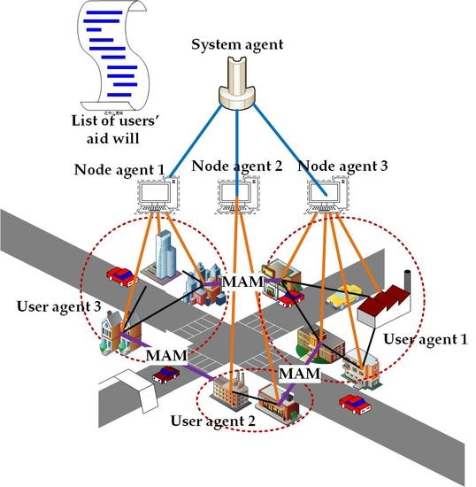
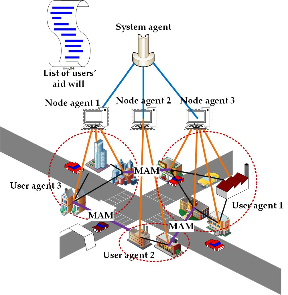
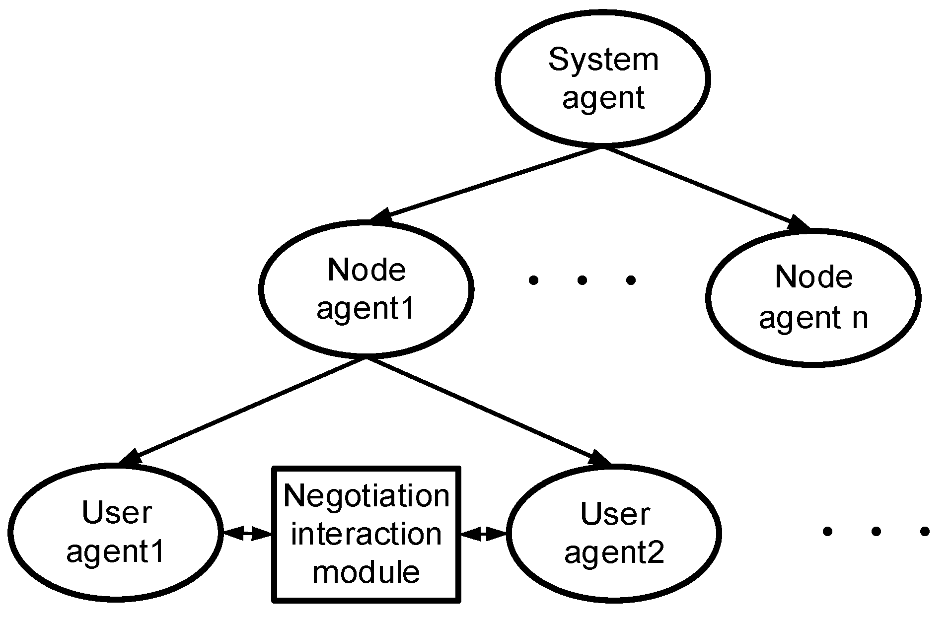
2.1. System Architecture

According to the physical structure, a power grid is divided into three layers, “system-node-user”. The node contains multiple users, while the system includes all nodes in the power grid. Then, the IMAS is established for the system, node and user to create the mathematical model. Finally, through interactions among agents, the allocation of the OPU gap indicators is completed. The structure is shown in Figure 1.

The functions of different levels of agents are designed as follows:

(1)

The system agent is responsible for calculating the system gap index. First, it collects the energy-saving characteristics of the subordinate nodes (including energy-saving potential and energy-saving loss coefficient) from each node agent. Then, according to the energy-saving characteristics, it calls the orderly allocation algorithm of the power gap index. Finally, the gap index is allocated to each node agent.

(2)

First, the node agent reports energy-saving characteristics to the system agent. Secondly, after getting the allocated gap indicators from the system agent, the node agent collects the energy-saving characteristics from the subordinate user agents and then, assigns the gap indicators to the user agents.

(3)

The user agents are the lowest layers in a IMAS. It abstracts the user and collects the user’s energy-saving features and reports them to the node agent.

(4)

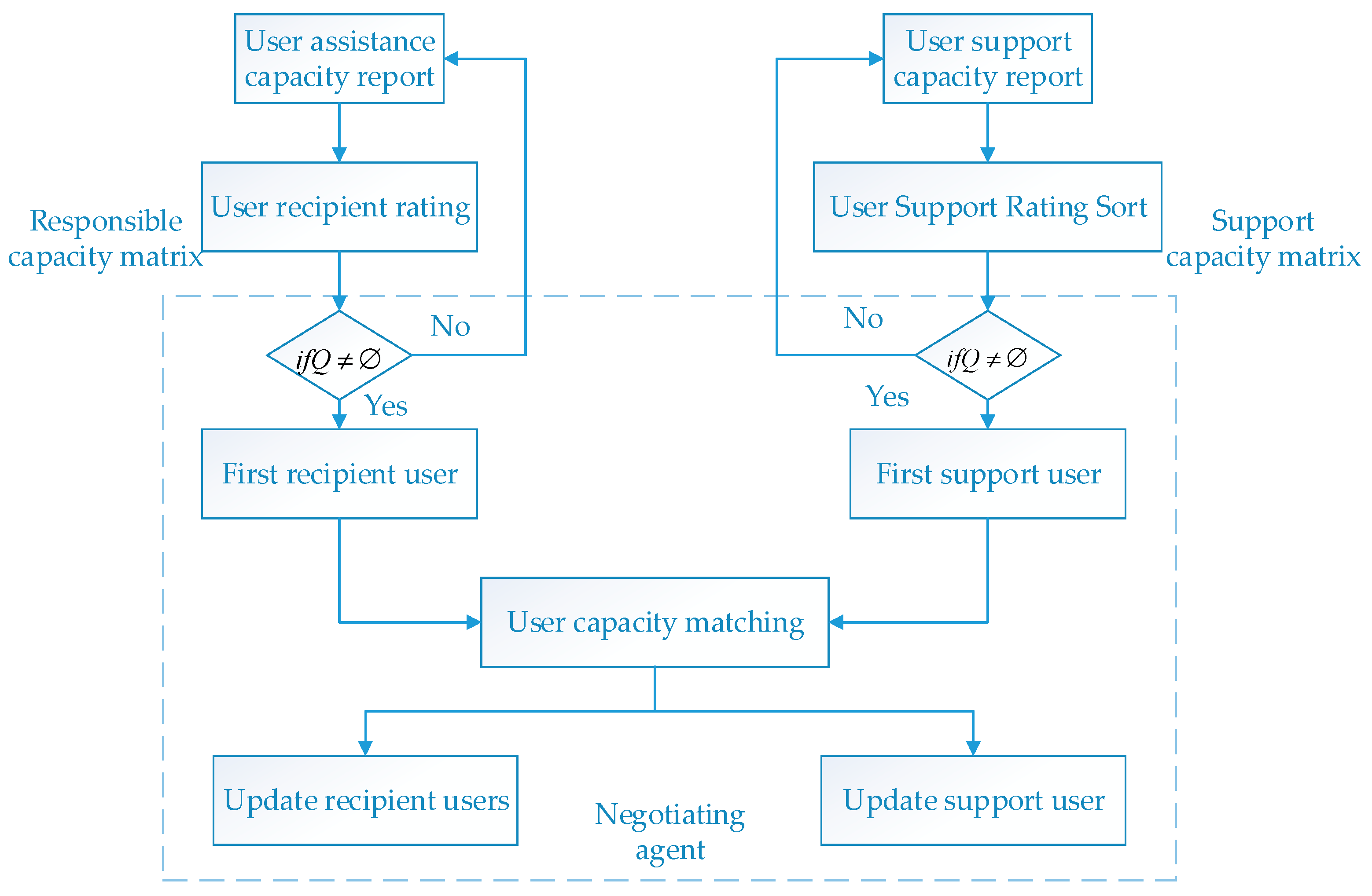
In the interactive module, the negotiation agent first collects the aid willingness of users to form a list. When a user is unable to perform the tasks as planned, the user agent can issue an aid request on the interactive platform. After querying the request, the negotiation agent quickly adjusts the OPU plan according to the user’s aid willingness table. Then the agent updates the table according to the aid situation to ensure the fairness of electricity consumption.

2.2. Indicator Distribution Mechanism

The OPU scheme adjusts at any time based on the user’s electricity consumption behavior. The scale of the distribution network is huge, and communication is hindered if it is repeatedly adjusted [21]. Insufficient interaction between users leads to a waste of energy and investment. Therefore, a user MAM that encourages mutual assistance is proposed. It reduces the pressure of system communication, improves the efficiency of solving large-scale planning problems, and ensures real-time information updates as follows:

(1)

Each layer of agent reports the energy-saving feature to the upper layer agent, and the upper layer agent summarizes the equivalent energy-saving characteristics;

(2)

After obtaining the energy-saving characteristics of the lower layer agent, the upper layer agent completes the gap index assignment task from the upper level to the lower level according to the allocated OPU gap indicator.

The key to MAM is that each user submits real energy-savings potential, then encourages users to respond to the aid requests of other users. With respect to prompting users to submit the real potential of energy-savings, it establishes an aid scoring mechanism for users. The user’s aid score is set as the total contribution in the historical aid task. The scores of users who contribute more are high. MAM is shown in Figure 2.

The receiving assistance user i submits $Q_i$ to the negotiation agent, and ranks the recipient users according to $W_i$. According to this order, $Q_i=\left[Q_1,Q_2,Q_3\dots Q_m\right]$ is obtained. Users with high scores get aid first, so $Q_1$ gets aid first, followed by $Q_2$, and finally $Q_m$.

3. I-CFSFDP

3.1. CFSFDP Algorithm

The idea of CFSFDP is based on the following two points: (1) the local density of each clustering center is higher than the density of its domain sample points and (2) the distance between the clustering center and the sample point with a higher density is relatively large. The point is defined as Equation (1) [27].

$${\rho }_i=\{\begin{array}{c}{\displaystyle {\displaystyle \sum }_j}(d_{ij}-d_c),x<0\\ 0,x\ge 0\end{array}$$

(1)

In Equation (1), $d_c$ has a great impact on the clustering effect. If $d_c$ is too small, it can cause a cluster to be forced to split into several parts; if $d_c$ is too large, several clusters can be merged into one class. In the $d_c$ range of the average sample point, $d_c$ should make the ratio of the sample size to the data set τ (τ = 1–2%) [17]. To reduce the influence of truncation distance on clustering results, we propose to improve ${\rho }_i$ by using the Gauss kernel function.

$${\rho }_i={\displaystyle \sum }_{j\ne i}\exp \left(-\frac{d_{ij}^2}{d_c}\right)$$

(2)

The minimum distance between each sample point and a point with a higher density is defined as follows:

$${\delta }_i=\underset{j:{\rho }_j>{\rho }_i}{\min }\left(d_{ij}\right)$$

(3)

In Equation (3), for the sample i whose density is the highest, ${\delta }_i=ma{x}_j\left(d_{ij}\right)$.

The CFSFDP algorithm does not consider the local structure of datasets when calculating $\rho$. When the density difference among different clusters of datasets is large, it will lead to wrong clustering (merging of several clusters or splitting of one cluster). If the dataset size is n, the internal memory consumption of the CFSFDP algorithm is mainly used to store a distance matrix of size $n\times n$. The execution time is mainly used to calculate the distance matrix, $d_c$, $\mathsf{\rho }$ and $\mathsf{\delta }$. The ratio of calculating the distance matrix is the largest, especially when the data scale and dimension are large. The internal memory consumption and execution time of the CFSFDP algorithm will increase rapidly with an increase of data size. Therefore, application of the CFSFDP algorithm is limited by data size, and it is not appropriate for high-dimensional massive load curve clustering analysis.

3.2. I-CFSFDP Algorithm

3.2.1. KNN Algorithms and Their k-d Tree Implementation

The KNN algorithm is a simple and practical supervised learning classification method, which is widely used in clustering analysis, prediction analysis, and pattern recognition [28]. There are two ways to implement the KNN algorithm which include: (1) Linear scan, which calculates the distance among each sample to be classified and all training samples. However, it takes a lot of time to implement a large number of high-dimensional training sets [29] and (2) store training data through special structures to reduce the number of calculated distances. One of the efficient classical methods is k-d tree [30]. The k-d tree is a kind of tree data structure that stores instance points in k-dimensional space for fast retrieval. The k-d tree is used to divide the k-dimensional search space, and the KNN samples can be obtained by a correlative search in the neighborhood space of the sample, thus avoiding exhaustive search calculations and greatly reducing the number of search calculations.

3.2.2. Principal Component Analysis for Dimension Reduction

Dimension reduction technology is mainly divided into feature selection and feature extraction. The feature selection selects feature subsets that contain most of the information of the dataset from the original redundant feature set [31]. However, the existing original feature subset cannot fully reflect the time characteristics of the load curve. The selected feature subset loses more information on the load curve [32]. Through transformation, feature extraction transforms the original high-dimensional feature space into a new low-dimensional feature space. Compared with other dimensionality reduction methods, principal component analysis (PCA) has the highest clustering accuracy and efficiency [33]. PCA is an important linear dimension reduction method. Its basic idea is to transform p original variables into m new orthogonal variables (m ≪ p) after linear transformation [34].

3.3. Improvement of the CFSFDP Algorithm

According to the literature [17,27,35], these study have mainly improved the internal memory consumption and execution time of the original algorithm. The PCA is used to reduce the dimension of the normalized load curve set. To speed up the follow-up operation, we first calculate the Euclidean distance. Then the KNN matrix is generated by a fast KNN search for dimension reduced data using the k-d tree algorithm. Finally, the KNN matrix is used to replace the distance matrix of the original algorithm as the input data. On the basis of the improved KNN criterion for calculating local density and distance of samples, the load curve is clustered by CFSFDP.

1. Improvement of internal memory consumption in the CFSFDP algorithm

CFSFDP cannot consider the local structure of the dataset when calculating the local density of the sample [36]. Therefore, the local density calculation standard introduces the idea of KNN and ${\rho }_i$ is defined as follows:

$${\rho }_i={\displaystyle \sum }_{j\in KNN\left(i\right)}\exp (-d_{ij}^2)$$

(4)

In the formula, Equation (4) shows that ${\rho }_i$ decreases with the increase of the distance from sample i to k- nearest neighbors. The new ${\rho }_i$ only considers the KNN sample, which reflects mostly the local structure of sample i. To reduce the internal memory consumption of the CFSFDP algorithm, we use KNN to improve the calculation criterion of sample distance. Except for some sample points (such as cluster centers), there is at least one nearest neighbor sample with a density higher than the density of the sample point i, the minimum distance ${\delta }_i$ of the sample point i and the point at which the density is higher is to be found from the k neighbor samples. Therefore, the improved ${\delta }_i$ based on KNN is defined as follows:

$${\delta }_i=\{\begin{array}{c}\underset{\left\{j\in KNN\left(i\right)\right\}\wedge \left\{{\rho }_j>{\rho }_i\right\}}{min}\left(d_{ij}\right)\\ if\exists js.t.\left\{j\in KNN\left(i\right)\right\}\wedge \left\{{\rho }_j>{\rho }_i\right\}\\ \underset{j:{\rho }_j>{\rho }_i}{min}\left(d_{ij}\right)\\ otherwise\end{array}$$

(5)

For the sample point i with the highest local density in the whole world,

$${\delta }_i=\underset{j\ne i}{\max }\left({\delta }_i\right)$$

(6)

k is obtained by Equation (7). The $\rho$ and $\mathsf{\delta }$ of the samples are calculated based on the KNN algorithm.

$$K=p\times n$$

(7)

Equation (7) shows that the proportion of KNN sample to the whole data scale is p, p is generally minimal, then i < n. The improved procedure for calculating sample distance $\delta$ is as follows:

(1)

The local sample density of the dataset is sorted in descending order and set to ${\rho }^{\prime }=({\rho }_1^{\prime }$, ${\rho }_2^{\prime }\dots {\rho }_n^{\prime })$, so that i = 2.

(2)

Calculate the distance ${\rho }_i^{\prime }$ of density ${\delta }_i^{\prime }$ according to Equation (5), i = i + 1.

(3)

If i $\le$ n, return to step (2); otherwise, i = 1. The distance ${\delta }_i^{\prime }$ corresponding to the density ${\rho }_i^{\prime }$ is calculated according to Equation (6).

2. Improvement of CFSFDP algorithm execution time

It is very time-consuming to use the linear scanning method to build the KNN matrix on large-scale datasets, and the classical k-d tree algorithm can realize a fast KNN search to create KNN matrix [37]. Because the KNN search efficiency is high when the size of the training set is much larger than the spatial dimension ($n\ge k$). The dimension increment causes a deviation of similarity measure and reduces the clustering effect [38]. To reduce the execution time of the CFSFDP algorithm, we first reduce the dimension of the dataset by PCA, then, use the k-d tree algorithm to establish the KNN matrix, and then, use Equations (4)–(7) to calculate the samples’ $\rho$ and distance $\mathsf{\delta }$.

3.4. I-CFSFDP Algorithm Step

The input of the load curve dataset is X, and the output of KNN proportional parameter p is a clustering result. The whole process of the I-CFSFDP algorithm is as follows:

(1)

The dataset X is normalized. This treatment fully reflects the morphological characteristics of each load curve, avoiding the influence of dimension and amplitude difference on the load curve clustering.

$$x_t^{\prime }=\frac{x_t-x_{min}}{x_{max}-x_{min}}$$

(8)

(2)

The normalized dataset is dimensionally reduced by PCA to ${\mathit{X}}^{*}$;

(3)

The KNN matrix of ${\mathit{X}}^{*}$ is established by the k-d tree algorithm.

(4)

Calculate the $\rho$ and $\mathsf{\delta }$ of samples according to Equations (4)–(7);

(5)

Since the difference between the order of magnitude $\rho$ and $\delta$ makes the weights of the two different, the first $\rho$ and $\delta$ are normalized, and the resulting decision curve avoids this problem. The larger $\mathsf{\gamma }$ point is selected as the cluster center.

(6)

The remaining samples are assigned, and each sample belongs to the same category as the denser and closest sample.

4. OPU Model Considering DSM

4.1. Establishment of Objective Function Model

From the perspective of the power grid, the objective is to minimize the total cost of OPU control.

$$min{\displaystyle \sum }_{i\in N}{\lambda }_i\left[C_i^{rotate}+{\displaystyle \sum }_{k=1}^7(C_{i,k}^{shift}+C_{i,k}^{clip}+C_{i,k}^{stag})\right]$$

(9)

From the user’s point of view, the goal is to minimize the total electricity cost of the user and promote the local consumption of PV power generation.

$$min{\displaystyle \sum }_{k=1}^7{\displaystyle \sum }_{i\in N}{\displaystyle \sum }_{t\in T}f\left(t\right)P_{i,k}\left(t\right)+{\displaystyle \sum }_{k=1}^7{\displaystyle \sum }_{i\in N}{\displaystyle \sum }_{t\in T}g\left(t\right)Z_{i,k}\left(t\right)$$

(10)

In the formula, k is the number of days; $C_i^{rotate}$ is the control cost of sequential rest; $C_{i,k}^{stag}$, $C_{i,k}^{shift}$ and $C_{i,k}^{clip}$ are the control costs of peak staggering, peak shifting, and peak clipping, respectively; $Z_{i,k}\left(t\right)$ is the power injected into grid when the output power of PV is higher than the user’s consumption; and $g\left(t\right)$ is the price of PV grid-connected.

4.2. Load Regulation Model

1. Peak staggering means that the user avoids load peak periods by delaying or by delaying the power consumption time of one day.

$$C_{i,k}^{stag}=u_{i,k}^{stag}\left|h_i\right|{\xi }^{stag}$$

(11)

$$\Delta P_{i,k}^{stag}\left(t\right)=u_{i,k}^{stag}\Delta P_i^{stag}\left(t\right)$$

(12)

where $i\in N$; $h_i$ is the number of hours of peak staggering in a time interval; $h_i$ is a positive number indicating the number of hours of peak staggering, and the negative number indicating the number of delays; $u_{i,k}^{trans}$ is 0–1 variable, and 1 is the number of peak staggering in a time; ${\xi }^{stag}$ is the correction amount of peak staggering in a time interval of t for i-user; $\Delta P_i^{stag}\left(t\right)$ is the number of peak staggering correction in a time interval of t-period for i-user; and $\Delta P_{i,k}^{stag}\left(t\right)$ is the correction of peak staggering for i-user at t-period on k-day.

2. Peak shifting and valley filling mean that the user shifts part of the load during peak hours to the valley period.Users need to submit the type and period of participation in peak shifting and valley filling.

$$C_{i,k}^{shift}={\displaystyle \sum }_{\beta =1}^{{\beta }_{max}}\left(\frac{1}{2}{u}_{i,k,\beta }^{shift}{\displaystyle \sum }_{t=1}^T\left|\Delta P_{i,\beta }^{shift}\left(t\right)\right|{\xi }_{\beta }^{shift}\right)$$

(13)

$$\Delta P_{i,k}^{shift}\left(t\right)={\displaystyle \sum }_{\beta =1}^{{\beta }_{max}}(u_{i,k,\beta }^{shift}\Delta P_{i,\beta }^{shift}\left(t\right))$$

(14)

where $i\in N$; $\mathsf{\beta }$ is the type of peak shifting valley filling; ${\beta }_{max}$ is the total number of peak shifting valley filling classes; ${\xi }_{\beta }^{shift}$ is the control cost coefficient of peak shifting valley filling; $u_{i,k,\beta }^{shift}$ is 0–1 variable, taking 1 as a variable to participate in the peak shifting valley filling of $\mathsf{\beta }$ class; $\Delta P_{i,\beta }^{shift}\left(t\right)$ is the correction of i- user participating in the t- period of peak shifting valley filling of $\mathsf{\beta }$ class; and $\Delta P_{i,k}^{shift}\left(t\right)$ is the total amount of peak shifting for i-user at t-period on k-day.

3. Peak clipping summit brings irreparable power loss to users, only when the power supply gap cannot be eliminated by the first three means. The user states the peak clipping, the single-stage peak clipping and the period of the maximum tolerable peak clipping level.

$$C_{i,k}^{clip}={\xi }^{clip}{M}_{i,k}{\displaystyle \sum }_{t=1}^T\Delta P_i^{clip}\left(t\right)$$

(15)

$$\Delta P_{i,k}^{clip}\left(t\right)=M_{i,k}\Delta P_i^{clip}\left(t\right)$$

(16)

where $i\in N$; $\Delta P_i^{clip}\left(t\right)$ is the single-stage peak clipping correction of i-user in t-period; $\Delta P_{i,k}^{clip}\left(t\right)$ is the total peak clipping correction of i-user in k-day t-period.

4. Peak rotating is suitable for users with weekly-off. By changing working days and rest days, the peak load of the system can be avoided.

$$C_i^{rotate}=u_{i,6}^{work}(1-u_{i,7}^{work}){\xi }_1^{rotate}+u_{i,7}^{work}(1-u_{i,6}^{work}){\xi }_1^{rotate}+u_{i,6}^{work}{u}_{i,7}^{work}{\xi }_2^{rotate}(i\in N_1)$$

(17)

$$P_{i,k}\left(t\right)=\{\begin{array}{c}{u}_{i,k}^{work}{P}_i^{work}\left(t\right)+(1-u_{i,k}^{work})P_i^{rest}\left(t\right)\left(i\in N_1\right)\\ P_{i,k}^{resident}\left(t\right)\left(i\in N_2\right)\end{array}$$

(18)

where k is the number of days; u is a variable of 0-1, 0 is the rest day, and 1 is the control cost coefficient of a working day, ${\xi }_1^{rotate}$ and ${\xi }_2^{rotate}$ are for one day and two days, respectively; $P_i^{work}\left(t\right)$ is a load of a working day with weekly rest i-user in t-period; $P_i^{rest}\left(t\right)$ is a load of a rest day with weekly rest i-user in t-period; $P_{i,k}^{resident}\left(t\right)$ is a load of resident i-user in the k-day t-period; and $P_{i,k}\left(t\right)$ is a load of resident i-user in the k-day t-period after rotate days off.

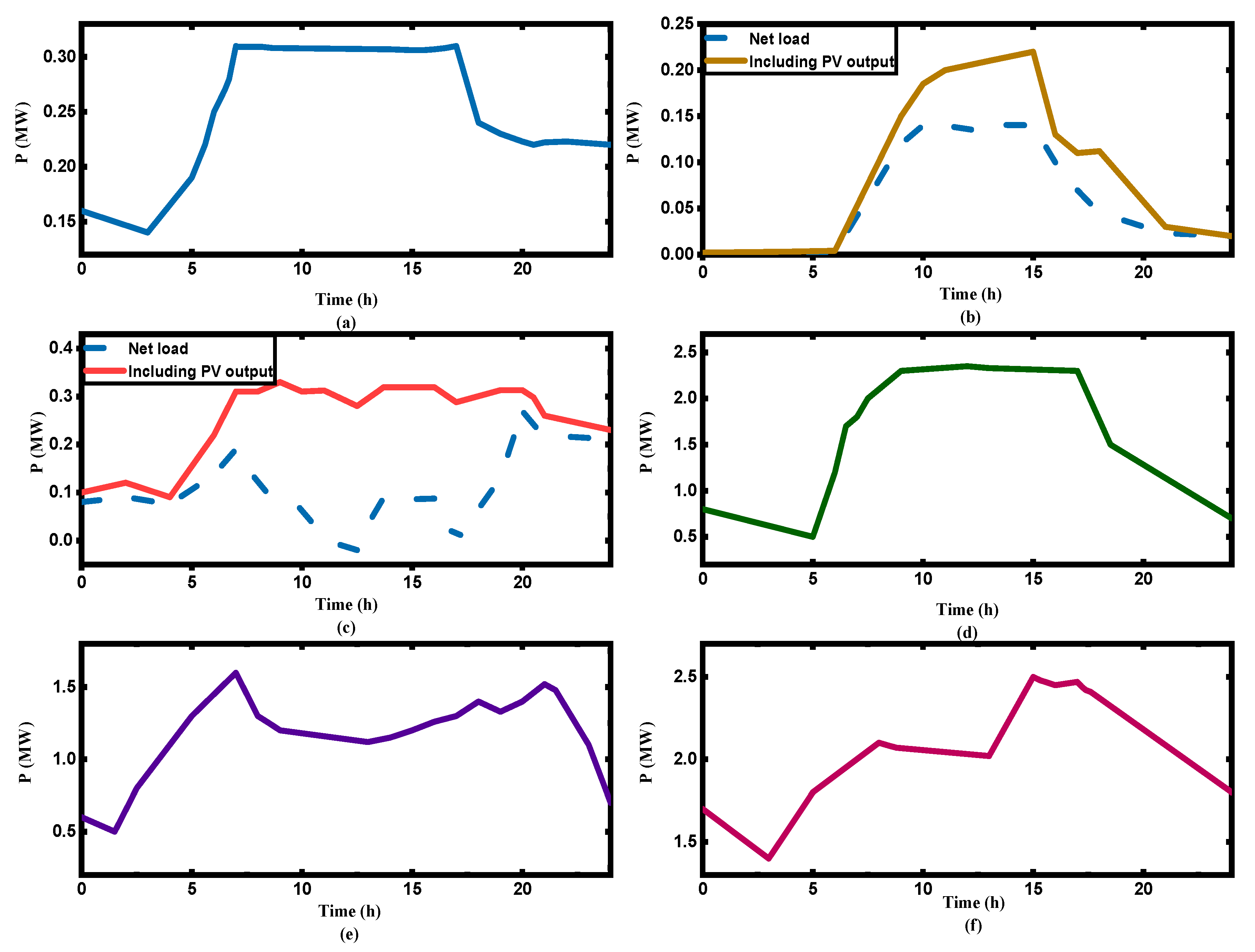
4.3. Modeling of Household PV Generation Devices

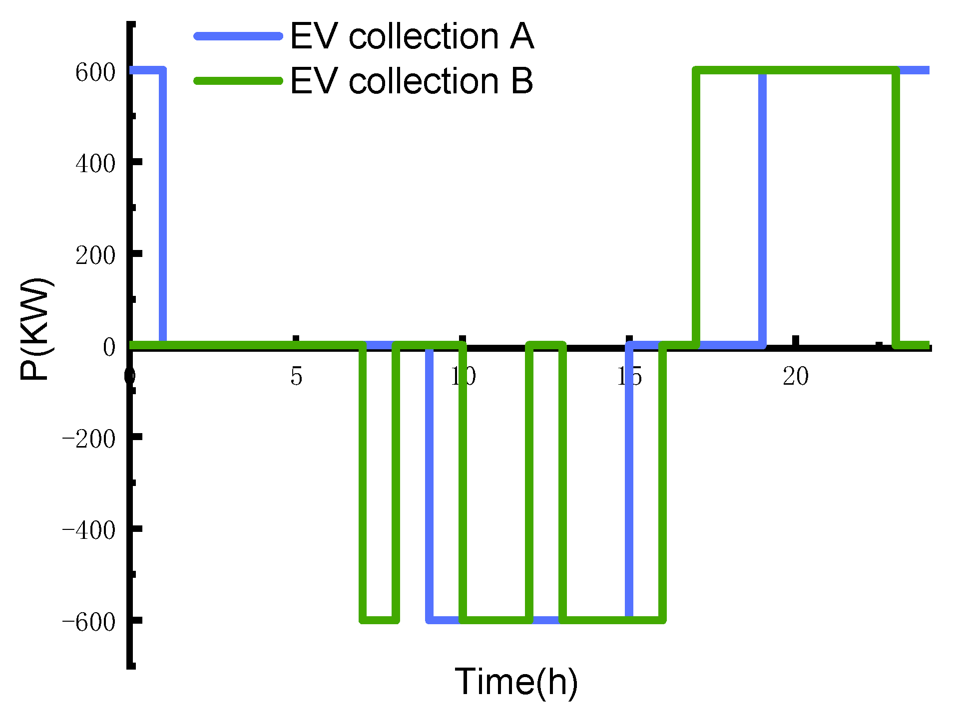
Household PV devices can directly supply power to users. The PV output power has strong nonlinear characteristics as a function of light intensity and temperature, and in cloudy weather, its output power will change rapidly for a short time [39].Its output power $P_{DC,k}\left(t\right)$ is affected by environmental factors [40]. The mathematical model is as follows:

$$P_{DG,k}\left(t\right)={\eta }_{DG}{S}_{DG}{K}_{DG}{n}_{DG}\left(1-0.005\left({\theta }_{out}^t-25\right)\right)$$

(19)

4.4. Modeling of EV

In the OPU scheme, the charging time can be adjusted to achieve the purpose of peak shifting and valley filling. The EV real power profile is not constant and strongly depends on the type of EV and the type of EV supply equipment [5,39,40]. Users need to declare the number of EVs available for a call and the adjustable charging time. The mathematical model of EV charging is as follows:

$$P_{EV}\left(t\right)=P_{EV}{S}_{EV}\left(t\right)$$

(20)

$${\mathrm{S}}_{EV}\left(\mathrm{t}\right)=\{\begin{array}{c}0,\left(Q_t\ge Q_{max}\right)\\ 1,(Q_t<Q_{max})\end{array}$$

(21)

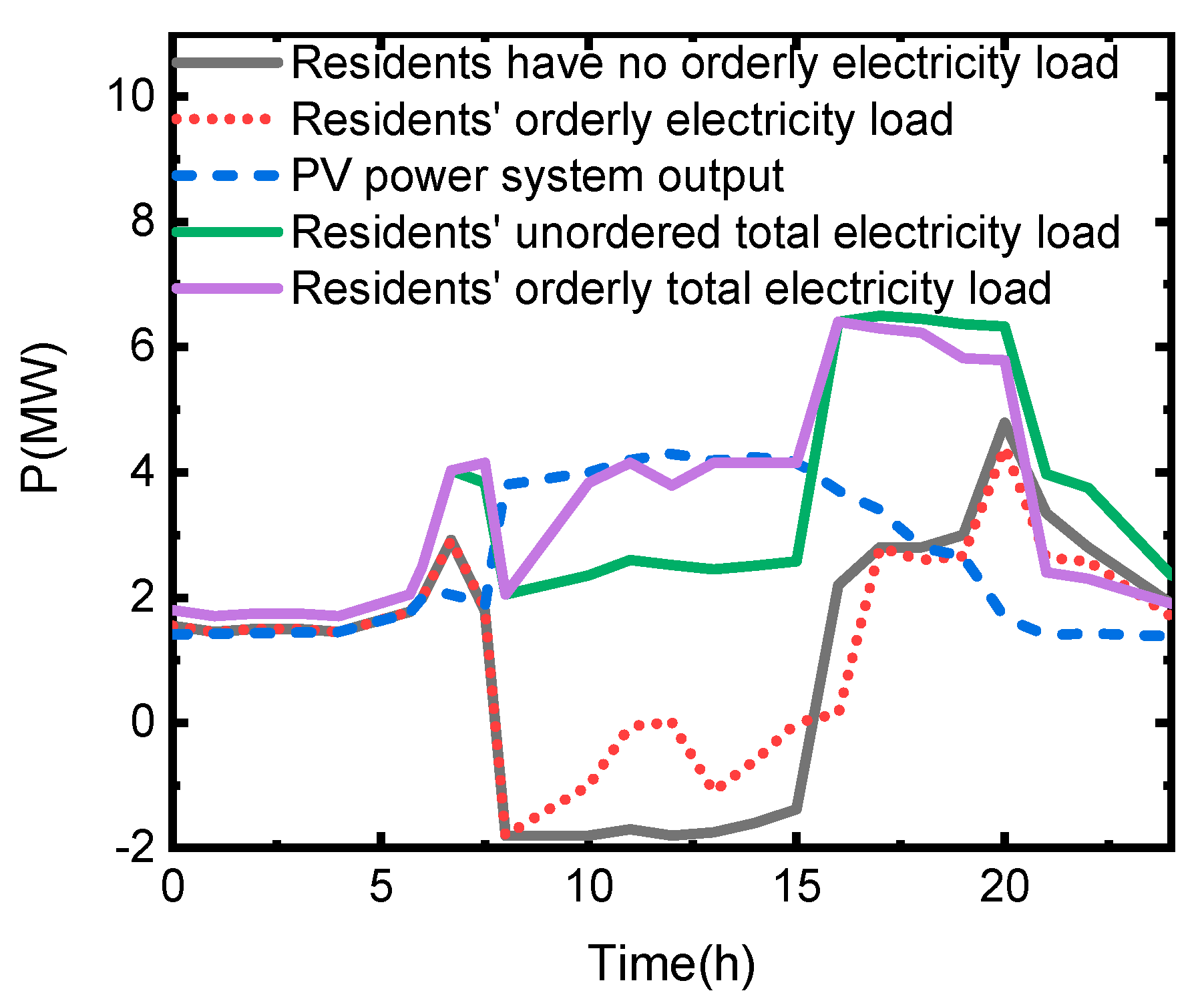
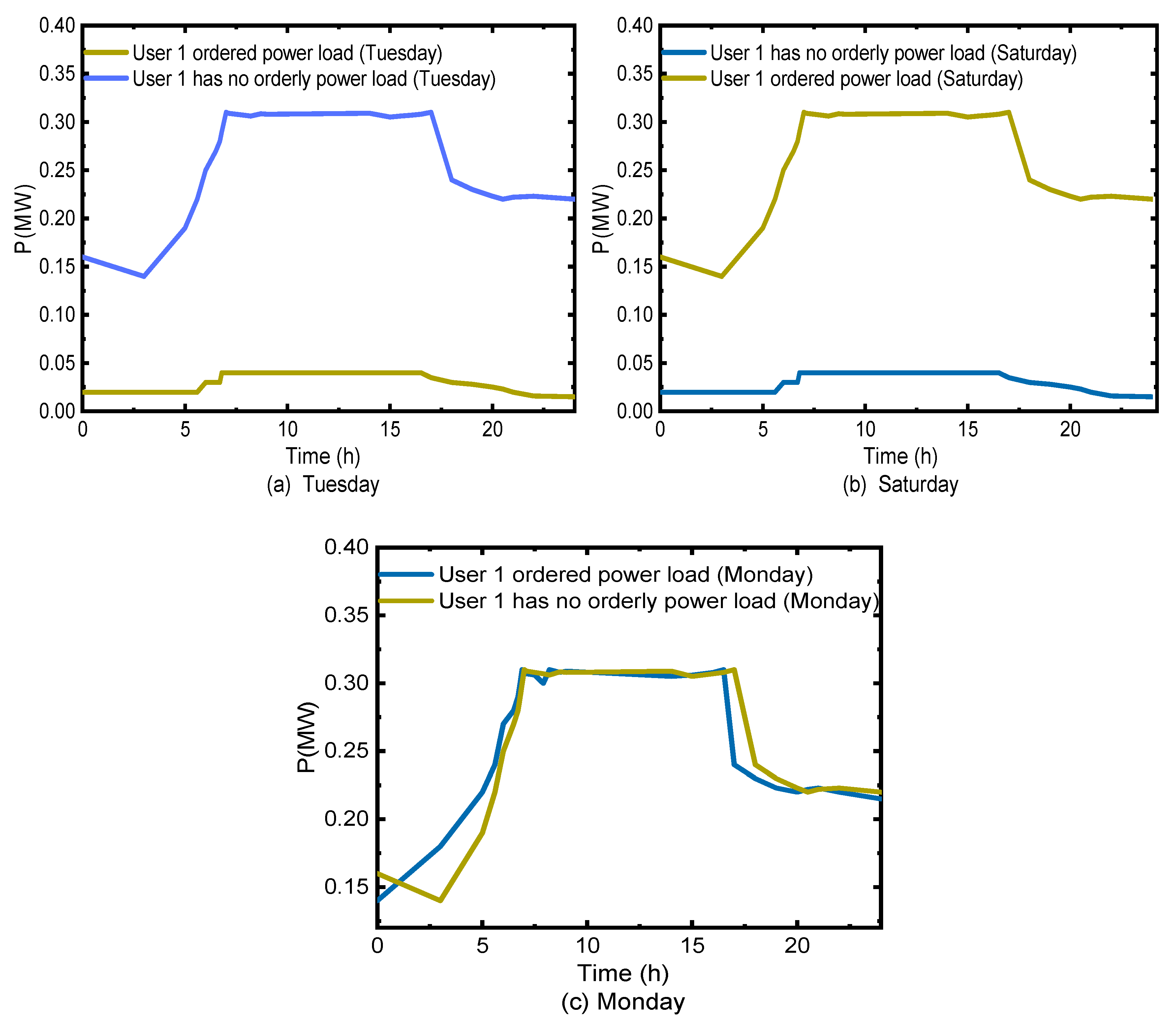
4.5. User Load Curve after OPU

After implementing the ordered power consumption strategy, the user’s power load curve is:

$$P_{i,k}\left(t\right)=\epsilon \left(P_{i,k}\left(t\right)-\Delta P_{i,k}\left(t\right)-P_{DG,k}\left(t\right)\right)$$

(22)

$$\Delta P_{i,k}\left(t\right)=\Delta P_{i,k}^{trans}\left(t\right)+\Delta P_{i,k}^{shift}\left(t\right)+\Delta P_{i,k}^{clip}\left(t\right)$$

(23)

$$Z_{i,k}\left(t\right)=\{\begin{array}{c}0(P_{DG,k}\left(t\right)<P_{i,k}\left(t\right))\\ P_{DG,k}\left(t\right)-P_{i,k}\left(t\right)(P_{DG,k}\left(t\right)>P_{i,k}\left(t\right))\end{array}$$

(24)

In the formula, $P_{i,k}\left(t\right)$ is the load of the user in the first k-day t-period after OPU, and the positive part of PV output is subtracted. When the value of $P_{i,k}\left(t\right)-\Delta P_{i,k}\left(t\right)-P_{DG,k}\left(t\right)$ > 0, $\Delta P_{i,k}\left(t\right)$ is the total OPU correction of the user in the t-period on the first day.

4.6. Constraints Condition

(1)

Maximum output constraints of the system

$${\displaystyle \sum }_{i=1}^N{P}_{i,k}\left(t\right)\le P_{G,k}^{max}$$

(25)

(2)

Constraints of peak shifting and peak clipping

$$h_{1max}\le h_i\le h_{2max}$$

(26)

$$M_{i,k}\le M_{max}$$

(27)

The number of hours of the peak staggering should not exceed $h_{1max}$ and $h_{2max}$ and the peak clipping level should not exceed the maximum tolerable level $M_{max}$.

(3)

Peak avoidance constraint

Each user uses at most one peak avoidance method one day.

$$u_{i,k}^{stag}+(1-u_{i,k,0}^{shift})+(1-u_{i,k}^{work})+u_{i,k}^{clip}\le 1\left(i\in N_i\right)$$

(28)

In the formula, $u_{i,k}^{stag}$ takes 1 to indicate that i-user participates in peak shifting on k-day; $u_{i,k,0}^{shift}$ takes 0 to indicate i-user participates in peak shifting and valley filling on k-day; $u_{i,k}^{clip}$ takes 1 to indicate i-user participates in peak clipping on k-day; $u_{i,k}^{work}$ takes 0 to indicate that i-user participates in peak shifting on k-day as a rest day.

(4)

The constraint of peak rotating

$${\displaystyle \sum }_{k=1}^7{u}_{i,k}^{work}=D_i\left(i\in N_1\right)$$

(29)

$D_i$ denotes the number of working days one week for the user. The above formula means that the total number of working days per user a week is fixed. Usually, $D_i=5$.

(5)

Daily participation restriction.

$$u_{i,k}^{stag}+(1-u_{i,k,0}^{shift})+u_{i,k}^{clip}\le 1\left(I\in N_2\right)$$

(30)

The meaning of the Formula (30) is that each user can only participate in one peak avoidance mode every day.

4.7. Solution Algorithm

The FSS can transform the multi-objective optimization problem into a single-objective solution, which sorts all the objectives according to the importance degree, first finds the optimal solution of the most critical objective, and then finds the next important objective [25,41]. It works the premise of guaranteeing the optimal solution of the former objective until the last one is obtained [42].

Solving m objects at the same time makes calculation difficult. First, the objects are ranked according to the importance of each object. The order of arrangement is:

$$h_1\left(x\right),h_2\left(x\right),h_3\left(x\right),\cdots h_m\left(x\right)$$

(31)

First, solve the first object $h_1\left(x\right)$ and find the set $R_1$ of the optimal solution; then, in $R_1$, solve the optimal solution $R_2$ of the second object $h_2\left(x\right)$; in $R_2$, solve the optimal solution $R_3$ of the third object $h_3\left(x\right)$. This continues until the optimal solution $R_m$ of the mth object $h_m\left(x\right)$ is obtained.

$$f_1\left(x^0\right)=ma{x}_{x\in R_1}^R{f}_1\left(x\right)$$

(32)

$$f_2\left(x^0\right)=ma{x}_{x\in R_2}^{R_1}{f}_2\left(x\right)$$

(33)

$$f_3\left(x^0\right)=ma{x}_{x\in R_3}^{R_2}{f}_3\left(x\right)$$

(34)

$$⋮$$

$$f_m\left(x^0\right)=ma{x}_{x\in R_m}^{R_{m-1}}{f}_m\left(x\right)$$

(35)

In the study, it can be considered that the object of to minimize the total cost of OPU control is more important, and the constraint is appropriately relaxed to solve the second object after solving the first object.After solving the objective Formula (9), the constraints should be relaxed to solve the objective Formula (10).

The OPU scheme in this study takes one week as the time unit, and combines it with the relevant parameters declared by users, preferentially calls low power value score users. The order of users’ load management mode calls is peak staggering, peak rotating, peak shifting and peak clipping. This process is equivalent to peak shifting and valley filling. For other users, the load of an EV has been considered in its peak shifting and valley filling load. The mathematical optimization solver CPLEX 12.4 is used to optimize the solution in Matlab.

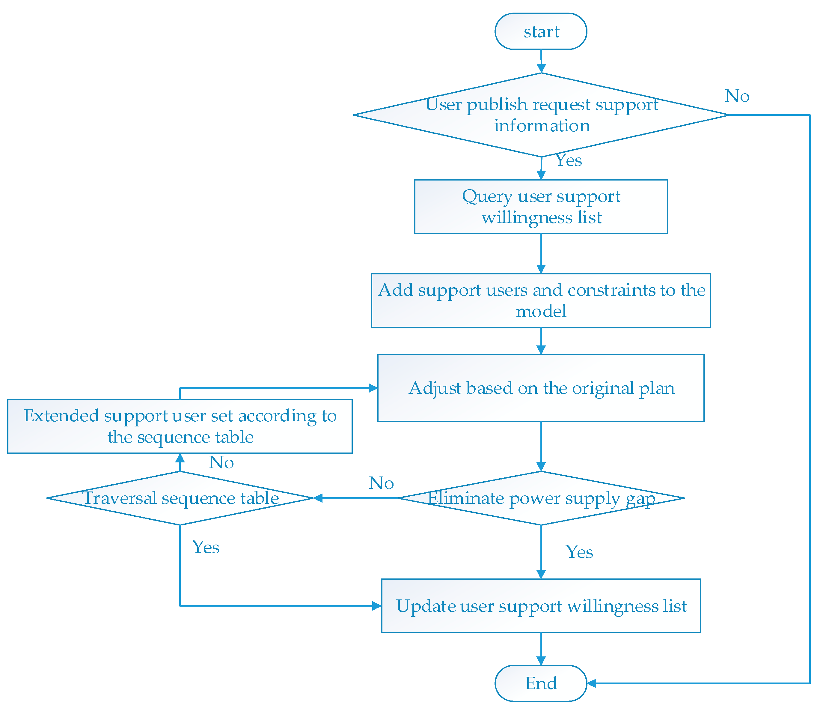
4.8. Adjustment of OPU Scheme

First, the user is ranked according to the degree of aid willingness to form a ranking table. When a user requests aid, the negotiation agent identifies the set of users that are preferentially responded to in the ranking order. If the set is not feasible, and the current adjustment capability is insufficient, the negotiation agent adds more users to the aid model one-by-one according to the sequence table. We can ensure that the adjustment cost is minimized based on the user’s willingness. The process of OPU adjustment is shown in Figure 3.

1. The negotiation agent inquires on the user interaction platform whether the user has issued an aid request, and if so, enters step 2.

2. Query the ranking table of user support intention, judge whether the user participates in the adjustment, construct the support user set, and add the corresponding constraints to the support model.

3. Make adjustments based on the original OPU scheme. The goal is to minimize the adjustment cost of the scheme as follows:

$$min{\displaystyle \sum }_{i\in Y}{\lambda }_i\left[C_i^{rotate}+{\displaystyle \sum }_{k=1}^7(C_{i,k}^{trans}+C_{i,k}^{shift}+C_{i,k}^{clip})\right]$$

(36)

4. Determine whether the power supply gap can be eliminated or not, if satisfied, update the user aid willingness ranking table and rank the users participating at the end of the ranking table in turn; if not, enter step 5.

5. Based on the original aid user set, add users one-by-one according to the sequence table, and update the aid model to step 3 until the sequence table is traversed.

5. Examples and Analysis of Planning Results

This study uses the commercial user load data published by the Open EI website of the U.S. Department of Energy. Each user includes 24 data every day.

The whole data includes 1600 summer workday load curves of 16 industry categories. The I-CFSFDP algorithm is used to clustering the sample set, as shown in Figure 4.

In Figure 4a,b,d, categories 1, 2, and 4 are single peak loads, which include office buildings (companies), schools and hospitals. These loads are mainly characterized by large daytime power consumption, a smooth load curve, and slight microwave fluctuation due to users’ rest load around 13:00. In the peak period, the duration of these three categories of load patterns is also slightly different. For example, the peak period of category 1 load is about from 7:00 to 17:00, which includes hospitals; the peak period of category 2 load is about from 9:00 to 16:00, which only includes warehouses; and the peak period of category 4 load is about from 9:00 to 17:00, which includes office buildings, schools and supermarkets. In Figure 4e, f, category 5 and 6 of loads have three peaks, which include hotels and restaurants. Among them, the difference in load forms of the categories 3 and 4 is shown in the time and duration of the peak period. In Figure 4c, the load peak appears at 7:00, 12:00, 18:00 and lasts about two hours. This category of load includes full-service restaurants, fast-service restaurants and small hotels. For example, category 5 of the load peak appears at 7:00, 18:00, 21:00 and lasts for a short time, which only includes large hotels. Category 6 of load is bimodal, which only includes apartments. The peak occurs at 8:00 and 19:00, and the peak period lasts about 2 h.

Categories 2 and 3 contain household PV devices and the rated capacity is about 4500 kW. The price of PV during sunny weather is $0.0713/(kW⋅h). The resident users have 1000 EVs with a rated charging power of 4 kW. They work during the day and charge after 18:00. It is assumed that 30% of EVs can participate in OPU, and the charging period can be adjusted to the daytime. The total load curve of the system in this region is the sum of all user load curves (except PV output). The peak load of a working day is about 38 MW, and the electricity price of each period is shown in

Table 2. Electricity price.

Time (h)	Electricity Price/($/(kW·h))
Valley time (0:00–7:00, 22:00–24:00)	0.051
Peak period (7:00–9:00, 14:00–16:00, 18:00–20:00)	0.13
Ordinary hours (9:00–14:00, 16:00–18:00, 20:00–22:00)	0.0977

.

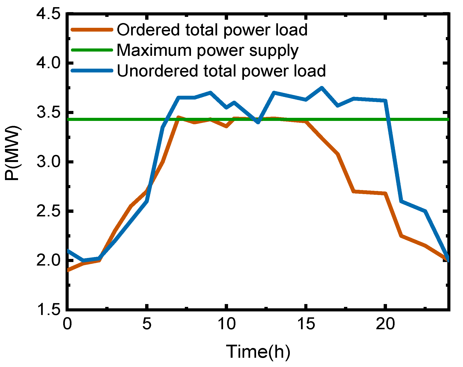
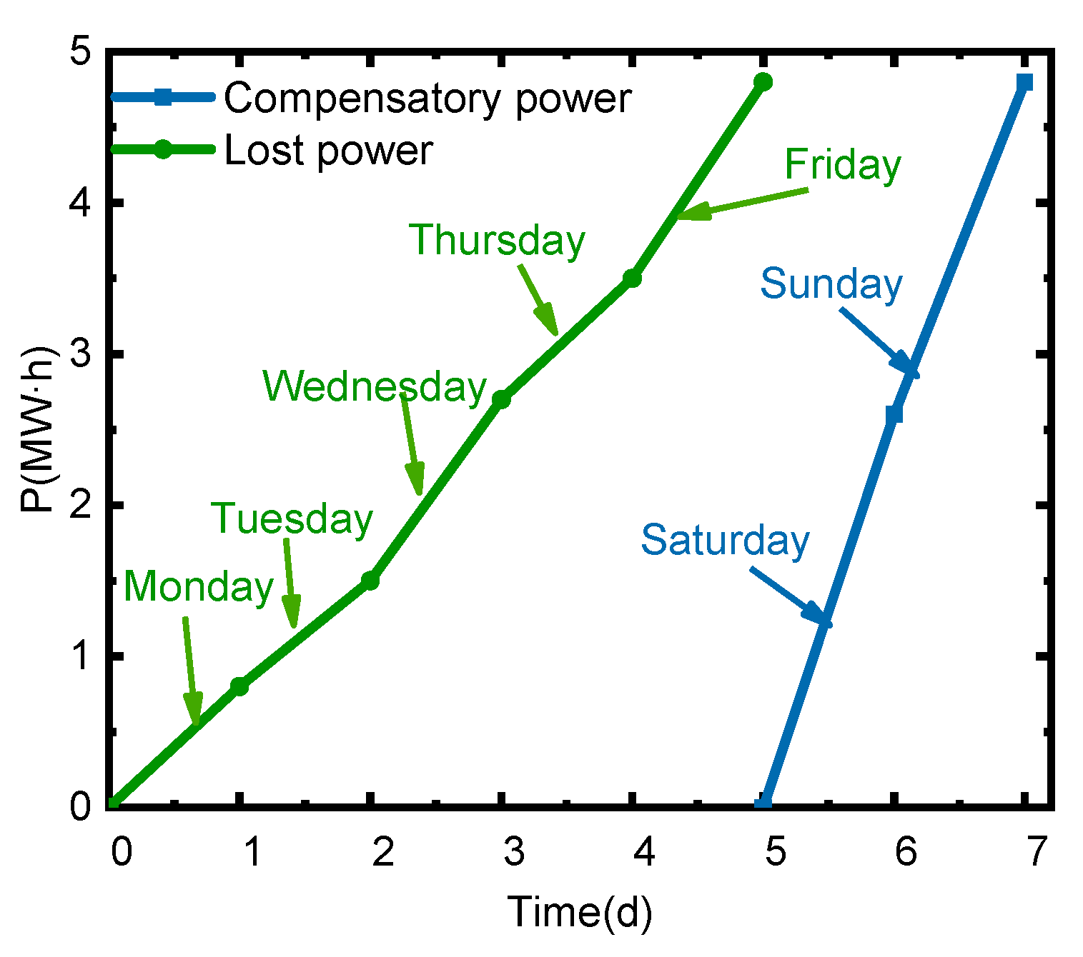
5.1. Scenario 1: In the First Week, the Region Was Allocated to Eliminate 10% of the Power Supply Gap, and the OPU Decision-Making Scheme in this Study Was Analyzed

If the traditional OPU is adopted (in the peak period, the user load is directly reduced regardless of the user’s will), and the power gap is 10%, the users’ categories 1, 4, 5 and 6 are called because of lower power value score. When each peak can be cut off, the peak clipping means of 11, 2, 16 and 5 are taken, respectively, and the total power loss reaches 67 MW·h, which affects the average demand of users. The decision results are shown in

Table 3. OPU decision-making scheme in this week.

User	Monday	Tuesday	Wednesday	Thursday	Friday	Saturday	Sunday
1	2 h	1 h	--	--	rest	rest	--
2	rest	--	--	--	--	rest	--
3	1 h	rest	--	--	--	--	rest
4	−2 h	--	--	−1 h	rest	--	rest
5	--	--	--	--	--	rest	rest
6	--	-	rest	--	--	rest	--

.

From Monday to Friday, all the resident users’ callable EVs participate in the OPU decision-making. Category 1, category 4, category 5 and category 6 take one day rotate days off, and category 1, category 4 and category 6 take the means of peak staggering periods for rotate days off. From the analysis of profitability, for power companies, they tend to give priority to users with low power value scores and use low-cost means. For users, they prefer the lowest total electricity cost if the load management method is adopted.

After OPU, the total load does not exceed the maximum supply and the power supply gap reduction. Figure 5 shows the total load curve of the system on Monday before and after OPU.

The change of the load curve in a week is shown in Figure 6.

After using the peak staggering mode, the power curve of category 1 is advanced 1 h, which reduces the peak load by 2621 kW at 16:00; the loss of electricity can be compensated in a day. In Figure 6a, the peak load on Tuesday is reduced by 4563 kW after using the rotate days off mode, and the loss of power can be compensated on Saturdays (Figure 6b).

EVs participate in peak shifting is shown in Figure 7.

The analysis of category 6 shows that before OPU, the charging arrangement of EV set A (150 EVs) concentrates between 19:00 and 1:00 the next day. After OPU, according to the user’s wishes, it transfers to between 9:00 and 15:00 for charging and EV set B (150 EVs) transfers to between 17:00 and 23:00 for charging. Charging is carried out from 7:00 to 8:00, 10:00 to 12:00, and 13:00 to 16:00. The peak load can be reduced by 1200 kW by the peak shifting and valley filling method, and the loss of electricity can be compensated for in a day. The condition of PV power plant consumption before and after the OPU is shown in Figure 8.

Before OPU, the net load of residential users is less than 0 from 8:00 to 15:00 and the PV output is not fully consumed. At 10:00, the waste of PV reaches a maximum, which is 1707 kW. As shown in Figure 8, when the EV participates in the OPU, the day net load curve changed significantly. The unabsorbed amount of 10:00 PV power decreased to 307 kW, and the total amount of PV power fed into the power grid decreased showing that an adjustment of the charging period for an EV can effectively promote the local consumption of distributed generation.

Electric quantity change after the OPU in this week is shown in Figure 9.

As shown in Figure 9, all users’ power losses from Monday to Friday can be compensated for on Saturdays and Sundays. The OPU mode ensures that the total power consumption of users will remain unchanged within a week. Through calculation, the savings for total electricity cost of users would be $1756.452 this week, and the grid could reduce the install capacity by approximately 3.8 MW.

5.2. Scenario 2: In the Process of Implementation, the User Needs to be Aided

1. First aid

In the third week, the region needs to eliminate 16% of the power supply gap. If category 1 cannot participate in OPU at this time to request aid, then, according to the user aid willingness list, add user 5 to the aid model and adjust the scheme. User 5 has made adjustments to Wednesday and Friday’s work schedule. On Wednesday, there are two types of peak shifting and valley filling, and on Friday, there are rotation breaks. According to the calculation, without OPU, user 1 wasted $272.494 of electricity cost, while user 5 saved $112.08 of electricity cost because of OPU. Subsequently, the aid willingness ranking table is updated to provide a reference for the next aid. The rotation situation is shown in

Table 4. User 1 and user 5 electrical modes before and after the adjustment.

Program	User	Monday	Tuesday	Wednesday	Thursday	Friday	Saturday	Sunday
Before adjustment	1	--	--	${\beta }_{12}$1	--	rest	rest	--
	5	--	--	--	--	--	rest	rest
After adjustment	1	--	--	--	--	--	rest	rest
	5	--	--	${\beta }_{12}$	--	rest	--	rest

¹ In Table 4, ${\beta }_{12}$ means participating in peak and valley shifting of the first and second categories.

.

2. Second aid

In the sixth week, the gap of power supply in this area is 8%, but user 3 cannot participate in the OPU. According to the sequence table, user 4 joins aid. The results show that the model has no solution, so it expands the available area of the aid user set, increases user 1 to aid model, and solves it again. The updated user aid willingness list provides a reference for the next aid.

3. After 12 weeks of OPU

The traditional aid method is to give priority to users with a low-value score or strong regulation ability, which lacks fairness. The aid method not only considers the willingness of users to aid but also takes turns to participate in the scheme adjustment. This method ensures the fairness of electricity consumption and realizes the coordination and autonomy of regional electric energy. The total electricity expenditure would be reduced by $12,816.91 in the summer. The number of users participating in aid is shown in

Table 5. Users’ participation times of aid.

User	Number of Aid for this Method	Number of Aid from Traditional Methods
1	1	0
2	0	0
3	1	2
4	1	5
5	2	0
6	1	0

.

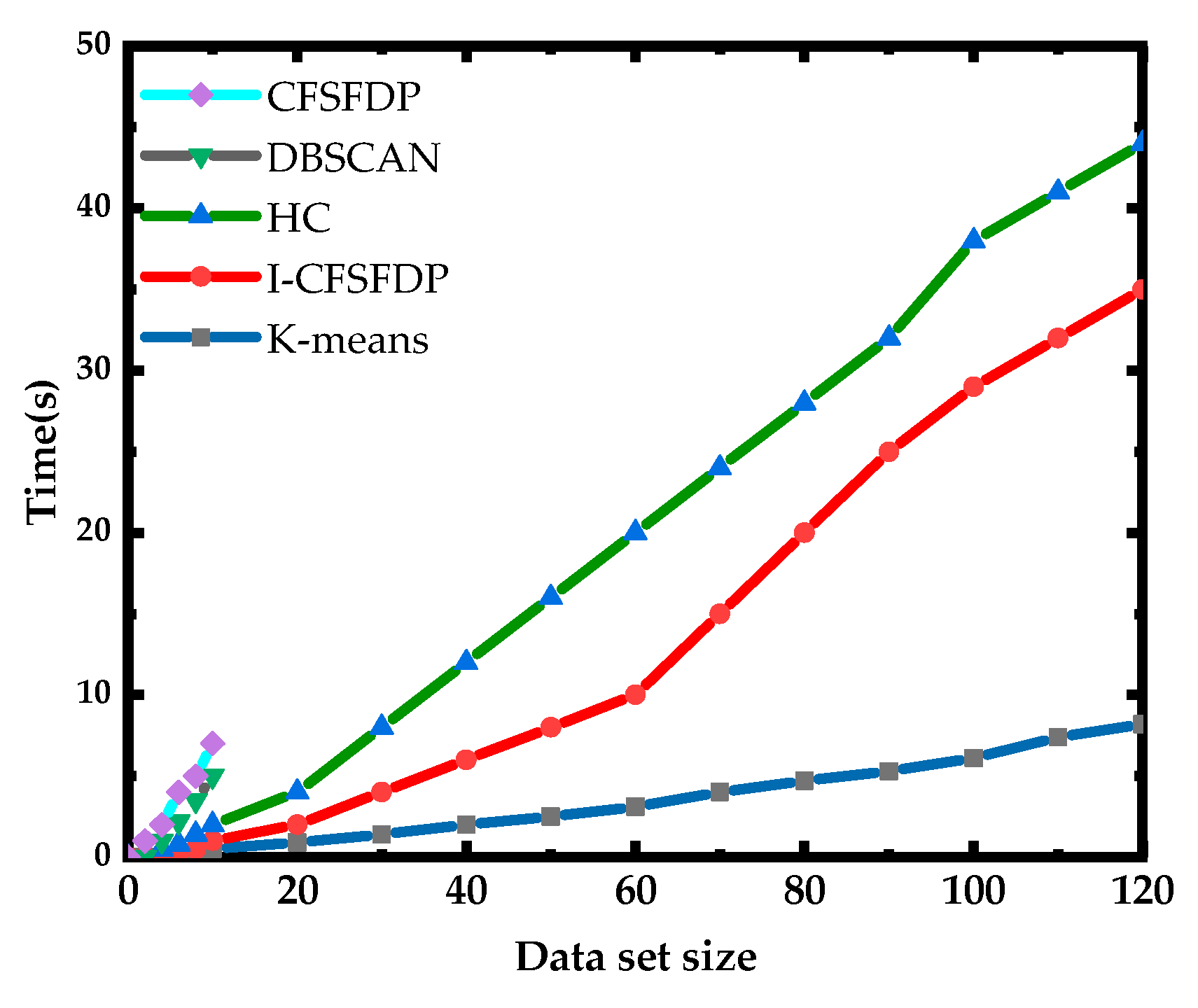
5.3. Comparison of Algorithm

Several traditional clustering algorithms and the I-CFSFDP algorithm are used for cluster analysis, and the overall internal memory consumption and execution time of each algorithm are compared. The experimental results are shown in Figure 10.

In terms of overall execution time, the I-CFSFDP algorithm is only worse than the k-means algorithm, which is better than the FCM algorithm and far better than other algorithms; in terms of overall internal memory consumption, the I-CFSFDP and FCM algorithms can handle datasets larger than 140,000. The rest of the algorithm has a memory overflow when the dataset size exceeds 8000, indicating that the internal memory consumption of the I-CFSFDP algorithm is within a reasonable range, which is much smaller than most clustering algorithms.

In summary, the internal memory consumption and execution time required by the I-CFSFDP algorithm are not high, far better than most traditional clustering algorithms, which verifies the applicability of the I-CFSFDP algorithm in high-dimensional massive load curve clustering analysis. Although the k-means algorithm is far superior to the I-CFSFDP algorithm, its clustering effect is poor and the results are unstable.

6. Conclusions

This study mainly focuses on OPU decision making under the mode of active user response. The active response and the potential of user response should be fully tapped. On the basis of IMAS technology, we propose an OPU scheme. The module divides the power grid into a three-tier agent structure of “system-node-user”. It separates the original complex OPU metrics into several simpler subtasks and encourages users to collaborate through proxy negotiation machines. The system realizes the second allocation of negotiation among user agents. By using the multilevel, adaptive and interactive allocation of the OPU gap index, when the first allocation of OPU index is inaccurate, users can adjust the gap index by the second optimization of the negotiation mechanism. Considering the user’s willingness and participation in peak avoidance, we analyzed the user’s electricity usage behavior.

The I-CFSFDP clustering algorithm is used to transform the uncertain model into a deterministic model. The clustering result is stable and productive. It also effectively reduces the internal memory consumption and execution time of the original algorithm. It better achieves large-scale power load curve clustering and assists load forecasting, price setting, and demand-side response in a big data environment.

On the basis of the the load characteristic curve obtained by the clustering algorithm, an M2OM is established. It aims to minimize the total cost of OPU control and the total cost of users’ power consumption. The model also promotes the local absorption of household PV. With high calculation efficiency, low-power score users’ wishes are respected. The model considers the interests of both users and the grid, as well as taps the user’s potential.

We propose an orderly adjustment method of OPU, which is realized by the negotiation agent, to achieve mutual coordination. In addition, we establishe an aid willingness ranking table to ensure fairness of power consumption. The OPU mode ensures that the total power consumption of users remains unchanged within a week. Through calculations, the total electricity cost savings for users in this region would be $1756.45 per week. In addition, the grid would reduce the installed capacity by approximately 3.8 MW. In summer, calculations show that the total electricity expenditure in this region would be reduced by $12,816.91. This study provides a reference for load management under the new situation of the smart grid. Power companies could reduce the imbalance between power supply and demand by implementing OPU decisions, alleviating the shortage of peak power and slowing the expansion of power plants.

OPU is a hot topic of current research. Possible research directions in the future should include charging load characteristics and orderly charging strategies for EVs, as well as optimal scheduling for integrating the energy system with power user-side participation.

References

1. Gellings, C.W. Evolving practice of demand-side management. J. Mod. Power Syst. Clean Energy 2017, 5, 1–9. [Google Scholar] [CrossRef]
2. Palensky, P.; Dietrich, D. Demand Side Management: Demand Response, Intelligent Energy Systems, and Smart Loads. IEEE Trans. Ind. Inform. 2011, 7, 381–388. [Google Scholar] [CrossRef]
3. Su, C.L.; Kirschen, D. Quantifying the effect of demand response on electricity markets. IEEE Trans. Power Syst. 2009, 24, 1199–1207. [Google Scholar]
4. Ahmed, N.; Levorato, M.; Li, G.P. Residential Consumer-Centric Demand Side Management. IEEE Trans. Smart Grid 2017, 9, 4513–4524. [Google Scholar] [CrossRef]
5. Han, S.; Han, S.; Sezaki, K. Development of an Optimal Vehicle-to-Grid Aggregator for Frequency Regulation. IEEE Trans. Smart Grid 2010, 1, 65–72. [Google Scholar]
6. Xiao, X.; Min, P.; Si, L. A Personalized Orderly Charging Strategy for Electric Vehicles Considering Users’ Needs. In Proceedings of the IEEE International Conference on Power System Technology, Guangzhou, China, 6–8 November 2018. [Google Scholar]
7. Hamed, S.G.; Kazemi, A. Multi-objective cost-load optimization for demand side management of a residential area in smart grids. Sustain. Cities Soc. 2017, 32, 171–180. [Google Scholar]
8. Chavali, P.; Yang, P.; Nehorai, A. A Distributed Algorithm of Appliance Scheduling for Home Energy Management System. IEEE Trans. Smart Grid 2014, 5, 282–290. [Google Scholar] [CrossRef]
9. Hadian, A.; Haghifam, M.R.; Zohrevand, J.; Akhavan-Rezai, E. Probabilistic approach for renewable DG placement in distribution systems with uncertain and time varying loads. In Proceedings of the IEEE Power & Energy Society General Meeting, Calgary, AB, Canada, 26–30 July 2009. [Google Scholar]
10. Zeng, B.; Zhang, J.H.; Yang, X.; Wang, J.H.; Dong, J.; Zhang, Y.Y. Intergrated planning for transition to low-carbon distribution systems with renewable energy generation and demand response. IEEE Trans. Power Syst. 2014, 29, 1153–1165. [Google Scholar] [CrossRef]
11. Kaloudas, C.G.; Ochoa, L.F.; Marshall, B.; Majithia, S.; Fletcher, I. Assessing the feature trends of reactive power demand of distribution networks. IEEE Trans. Power Syst. 2017, 32, 4278–4288. [Google Scholar] [CrossRef]
12. Shen, X.W.; Shahidehpour, M.; Zhu, S.Z.; Han, Y.D.; Zheng, J.H. Multi-stage planning of active distribution networks considering the co-optimization of operation strategies. IEEE Trans. Smart Grid 2018, 9, 1425–1433. [Google Scholar] [CrossRef]
13. Chicco, G.; Napoli, R.; Piglione, F. Comparisons Among Clustering Techniques for Electricity Customer Classification. IEEE Trans. Power Syst. 2006, 21, 933–940. [Google Scholar] [CrossRef]
14. Kanungo, T.; Mount, D.M.; Netanyahu, N.S. An efficient k-means clustering algorithm: Analysis and implementation. IEEE Trans. Pattern Anal. Mach. Intell. 2002, 24, 881–892. [Google Scholar] [CrossRef]
15. Azzag, H.; Venturini, G.; Oliver, A. A hierarchical ant based clustering algorithm and its use in three real-world applications. Eur. J. Oper. Res. 2007, 179, 906–922. [Google Scholar] [CrossRef]
16. He, Y.; Tan, H.; Luo, W. MR-DBSCAN: An Efficient Parallel Density-based Clustering Algorithm using MapReduce. In Proceedings of the IEEE International Conference on Parallel & Distributed Systems, Singapore, 17–19 December 2012. [Google Scholar]
17. Rodriguez, A.; Laio, A. Machine learning. Clustering by fast search and find of density peaks. Science 2014, 344, 1492. [Google Scholar] [CrossRef] [PubMed]
18. Pilevar, A.H.; Sukumar, M. GCHL: A grid-clustering algorithm for high-dimensional very large spatial data bases. Pattern Recognit. Lett. 2005, 26, 999–1010. [Google Scholar] [CrossRef]
19. Zhang, Y.; Brady, M.; Smith, S. Segmentation of brain MR images through a hidden Markov random field model and the expectation-maximization algorithm. IEEE Trans. Med. Imaging 2002, 20, 45–57. [Google Scholar] [CrossRef]
20. Davidson, E.M.; Mcarthur, S.D.J.; Mcdonald, J.R. Applying multi-agent system technology in practice: Automated management and analysis of SCADA and digital fault recorder data. IEEE Trans. Power Syst. 2006, 21, 559–567. [Google Scholar] [CrossRef]
21. Li, W.; Logenthiran, T.; Phan, V.-T.; Woo, W.L. Intelligent Multi-Agent System for Power Grid Communication. In Proceedings of the IEEE TENCON 2016-2016 IEEE Region 10 Conference, Singapore, 22–25 November 2016. [Google Scholar]
22. Wilkosz, K. Utilization of multi-agent system for power system topology verification. In Proceedings of the IEEE 2014 15th International Scientific Conference on Electric Power Engineering (EPE), Brno-Bystrc, Czech Republic, 12–14 May 2014. [Google Scholar]
23. Deng, R.; Yang, Z.; Chow, M.Y. A Survey on Demand Response in Smart Grids: Mathematical Models and Approaches. IEEE Trans. Ind. Inform. 2015, 11, 570–582. [Google Scholar] [CrossRef]
24. Farid, A.M. Multi-Agent System Design Principles for Resilient Coordination & Control of Future Power Systems. Intell. Ind. Syst. 2015, 1, 255–269. [Google Scholar]
25. Multazam, T.; Putri, R.I.; Pujiantara, M. Wind farm Site Selection Base On Fuzzy Analytic Hierarchy Process Method; Case Study Area Nganjuk. In Proceedings of the International Seminar on Intelligent Technology and Its Applications (ISITIA), Mataram, Indonesia, 28–30 July 2016. [Google Scholar]
26. Commercial and Residential Hourly Load Profiles for all TMY3 Locations in the United States. Available online: https://openei.org/doe-opendata/dataset/commercial-and-residential-hourly-load-profiles-for-all-tmy3-locations-in-the-united-states (accessed on 1 September 2014).
27. Wang, S.; Wang, D.; Li, C. Comment on “Clustering by fast search and find of density peaks”. arXiv 2015, arXiv:1501.04267. [Google Scholar]
28. Du, M.; Ding, S.; Jia, H. Study on Density Peaks Clustering Based on k-Nearest Neighbors and Principal Component Analysis. Knowl. Based Syst. 2016, 99, 135–145. [Google Scholar] [CrossRef]
29. Duch, A.; Jiménez, R.M.; Martínez, C. Selection by rank in K-dimensional binary search trees. Random Struct. Algorithms 2014, 45, 14–37. [Google Scholar] [CrossRef]
30. Cover, T.; Hart, P. Nearest neighbor pattern classification. IEEE Trans. Inf. Theory 1953, 13, 21–27. [Google Scholar] [CrossRef]
31. Kambhatla, N.; Leen, T.K. Dimension Reduction by Local Principal Component Analysis. Neural Comput. 1997, 9, 1493–1516. [Google Scholar] [CrossRef]
32. Baldi, P.; Hornik, K. Neural networks and principal component analysis: Learning from examples without local minima. Neural Netw. 1989, 2, 53–58. [Google Scholar] [CrossRef]
33. Tipping, M.E.; Bishop, C.M. Probabilistic Principal Component Analysis. J. R. Stat. Soc. 2010, 61, 611–622. [Google Scholar] [CrossRef]
34. Nomikos, P.; Macgregor, J.F. Monitoring batch processes using multiway principal component analysis. Aiche J. 2010, 40, 1361–1375. [Google Scholar] [CrossRef]
35. Bie, R.; Mehmood, R.; Ruan, S. Adaptive fuzzy clustering by fast search and find of density peaks. Pers. Ubiquitous Comput. 2016, 20, 785–793. [Google Scholar] [CrossRef]
36. Jiang, L.; Zhang, M.; Zheng, J. Optimization of clustering by fast search and find of density peaks. In Proceedings of the IEEE International Conference on Bioinformatics and Biomedicine (BIBM), Kansas City, MO, USA, 13–16 November 2017. [Google Scholar]
37. Wang, J.; Neskovic, P.; Cooper, L.N. Improving nearest neighbor rule with a simple adaptive distance measure. Pattern Recognit. Lett. 2007, 28, 207–213. [Google Scholar] [CrossRef]
38. Jégou, H.; Douze, M.; Schmid, C. Product Quantization for Nearest Neighbor Search. IEEE Trans. Pattern Anal. Mach. Intell. 2010, 33, 117–128. [Google Scholar] [CrossRef]
39. Pasetti, M.; Rinaldi, S.; Flammini, A. Assessment of Electric Vehicle Charging Costs in Presence of Distributed Photovoltaic Generation and Variable Electricity Tariffs. Energies 2019, 12, 499. [Google Scholar] [CrossRef]
40. Richardson, P.; Flynn, D.; Keane, A. Optimal Charging of Electric Vehicles in Low-Voltage Distribution Systems. IEEE Trans. Power Syst. 2012, 27, 268–279. [Google Scholar] [CrossRef]
41. Babich, O.A.; Pershin, O.Y.; Mushtonin, A.V. A Method to Design a Hierarchical Network of Field Pipelines by Solving a Sequence of Extremal Problems. Autom. Remote Control 2003, 64, 806–814. [Google Scholar] [CrossRef]
42. Song, Y.; Morency, L.P.; Davis, R. Action Recognition by Hierarchical Sequence Summarization. In Proceedings of the IEEE Conference on Computer Vision & Pattern Recognition, Columbus, OH, USA, 24–27 June 2014. [Google Scholar]
Figure 1. Intelligent multi-agent system (IMAS) for orderly power utilization (OPU).
Energies 12 04563 g001
Figure 2. Users’ mutual aid mechanism (MAM) encouraging users’ mutual support.
Energies 12 04563 g002
Figure 3. Flow chart of OPU scheme adjustment.
Energies 12 04563 g003
Figure 4. Users’ typical daily load curves: (a) Category 1 (200 users); (b) category 2 (100 users); (c) category 3 (300 users); (d) category 4 (800 users); (e) category 5 (800 users); (f) category 6 (100 users).
Energies 12 04563 g004
Figure 5. System load curve before and after OPU on Monday.
Energies 12 04563 g005
Figure 6. User 1 load curve before and after OPU: (a) User 1 Tuesday orderly load curve; (b) user 1 Saturday orderly load curve; (c) user 1 Monday orderly load curve.
Energies 12 04563 g006
Figure 7. Electric vehicles (EVs) participate in peak shifting (positive for peak removing, negative for valley filling).
Energies 12 04563 g007
Figure 8. Condition of photovoltaic (PV) power plant consumption before and after the OPU.
Energies 12 04563 g008
Figure 9. Electrical quantity change after the OPU in this week.
Energies 12 04563 g009
Figure 10. Performance comparisons between each clustering algorithm.
Energies 12 04563 g010