Thermal Diagnostics of Natural Ventilation in Buildings: An Integrated Approach

Abstract

Diagnostics of natural ventilation in buildings is problematic, as the airflow rate changes considerably over time. One constant average airflow is usually assumed when calculating energy demand for a building, however, such a simplification could be fraught with considerable error. The paper describes a comprehensive methodology for the diagnostics of a natural ventilation system in a building and its practical application. Based on in situ measurements and simulations in two existing buildings (dwelling house and school) in Poland, the real values of the ventilating airflows were analyzed and resulting heat demand was compared with the design values. The pros and cons of various methods for evaluation of natural ventilation are discussed. The real airflow was determined by measurements in a ventilation grille or by a tracer gas concentration decay method. The airtightness of the buildings’ envelope was evaluated based on the fan pressurization test. The last stage entailed computer simulations of air exchange in buildings using CONTAM software. The multizone models of the buildings were calibrated and verified with existing measured data. Measured airflow in a multifamily house was small and substantially deviated from the Polish standard. In case of a school, the air flow rate amounted to an average of 10% of the required value. Calculation of the heat demand for ventilation based on the standard value of the airflow led to a considerable overestimation of this value in relation to the real consumption. In the analyzed cases, the difference was 40% for the school and 30% for the residential building.

1. Introduction

Energy demand in the building sector is a significant component in the energy balance of every developed country, consisting of around 40% of world energy consumption [1,2]. Energy consumption depends on ambient temperature in the area of investigation and also on the season of the year, i.e., cooling and heating degree days [3]. Residential and public buildings in cold and moderate climates require a large amount of heat. With good insulation of the building’s external walls, the share of ventilation needs is well above 50% of total heat consumption [4,5].

Many buildings still use natural ventilation to remove polluted air from room. The assessment of energy consumption in buildings for ventilation purposes is difficult, especially if the building and systems are examined as a whole, and detailed phenomena related to the functioning of the system are ignored, as reported by Maile et al. [6].

The assessment of natural ventilation in buildings is often performed using numerical modelling. The accuracy of simulation models of ventilation has always been of interest, in terms of both the way the physical processes are reproduced and the accuracy of the calculations. Zhaia et al. [7] presented a critical review of computational and simulation models of natural ventilation. Their study shows that in typical, simple cases, numerical models correspond to real phenomena. This applies to the design and specification of ventilation airflow paths (windows, doors, cracks). Uncertainty in the numerical modelling of ventilation, for example in CONTAM [8], refers in particular to wind influence (wind profile, wind pressure coefficient, discharge coefficient). Li et al [9] present results of measurement and simulation of the airflow pattern inside the 5-story building equipped with natural ventilation under different wind conditions. Baranowski and Ferdyn-Grygierek [10] demonstrated the differences in the simulation results due to various complexities of the numerical model of residential and public buildings, i.e., the number of computational zones.

Research analyses of natural ventilation are often performed with advanced numerical simulation based on integrating the Computational Fluid Dynamics (CFD) method. Stavridou and Prinos [11] presented the results of such calculations performed with ANSYS Fluent software for cross ventilation and conducted complementary laboratory tests. The results of numerical calculations and laboratory measurements showed good convergence. Simulation results for cross ventilation and single-side natural ventilation models were compared with both aerodynamic tunnel test results and measurements in an existing building by Freire et al. [12]. There was a significant discrepancy in the results of the airflow calculations (over 30%) obtained both for three different natural ventilation models and in comparison with the experimental data. The authors suggest the need to improve empirical models for natural ventilation. Zhou et al. [13] responded to this suggestion and proposed a model of a single-side natural ventilation which gives results in a good agreement with transient simulation.

In publications on computational and simulation methods, the necessity of verification of the results of simulation calculations is strongly emphasized and often the validation of numerical models by data measured in real buildings are presented. Martins and Carrilho da Graça [14] showed that the use of CFD models gives an average error in airflow estimation of 25% compared to measurements. Assessment of natural ventilation in the apartment buildings by probabilistic approach is proposed by Hyun et al [15]. It is shown that uncertainty in both input data and simulation model may influence the prediction of air exchange in the apartments.

For the purpose of better evaluation of the building operation strategy Dols et al. [16] suggest integration of energy consumption simulation results and ventilation airflow in buildings. Aparicio-Fernández et al. [17] used the building energy performance modelling tools TRNSYS and TRNFlow to obtain the energy demand of a detached house that includes the air infiltration rate and the effect of natural ventilation by opening windows. Baranowski and Ferdyn-Grygierek [18] presented results of measurements of energy consumption and air exchange in a multifamily apartment during the heating season. Measurements were used to validate the simulation results with ESP-r (energy consumption) and CONTAM (air exchange) programs performed for the same period of time. Good agreement of air exchange measurements and the results of the simulation was obtained, although the measurement results were slightly higher than those from the simulation. The average relative error was approximately 5% for ESP-r and 12% for CONTAM results. The accuracy of air exchange results using different methods (analytical, empirical, simulation, and experimental models) was investigated by Omrani et al. [19].

In public buildings equipped with natural ventilation systems, the appropriate ventilation rate is based on adequate indoor air quality, considering the minimization of energy consumption. The same criteria apply for office buildings as well as for schools and museums. Ben-David and Waring [20] compared the results of energy consumption simulations and concentration of indoor air pollutants in a dozen office buildings located in different U.S. locations. Calculations were made for different ventilation strategies—natural, mechanical, and hybrid, resulting in similar concentrations of pollutants, but with lower energy demand for natural ventilation. Similar simulations were made by Popiolek and Ferdyn-Grygierek for a school building [5,21], showing the inefficiency of the natural ventilation system to ensure appropriate indoor air quality. Improving the efficiency of natural ventilation can be achieved by using a double-glazed facade. Such solutions result in both intensification of air exchange and improvement of thermal comfort inside the building. Comprehensive research into the effectiveness of such solutions for a typical office building is presented in [22].

Due to the time and manner of their usage, school buildings have a special characteristic of their utilization. This was highlighted by Mateus et al. [23] who presented a comparison of ventilation measurements and simulations in several classrooms. Mumovic et al. [24] pointed on an interesting aspect of indoor air quality in school buildings—the interaction between the dynamic behavior of occupants and the building ventilation system. The paper by Kim and de-Dear [25] presents the similar study but from the point of view thermal comfort. The effectiveness of ventilation and the energy demand are related to the requirements of good indoor air quality. According to ASHRAE standard [26] acceptable indoor air quality is “air in which there are no known contaminants at harmful concentrations as determined by cognizant authorities and with which a substantial majority of the people exposed do not express dissatisfaction.” CO₂ concentration is often used to assess indoor air quality. The acceptable value of CO₂ concentration in commercial rooms amounts to 1000–1200 ppm [26,27,28]. The problem of indoor air quality in buildings has gained importance as a result of changes in construction technology and introduction of new technological solutions enforced by updated standards limiting heat loss. For example, airtight windows are, on one hand, very desirable for energy efficiency, but on the other hand they limit the supply of outside air, often below the minimum hygiene criterion. Therefore, some modernization measures are associated with a deterioration of indoor air quality. An example of the energetic effects of thermomodernization of Polish school buildings can be found in the works of Ferdyn-Grygierek and Blaszczok [29], Ferdyn-Grygierek [5], and Popiołek and Ferdyn-Grygierek [21], where optimal solutions for energy savings are sought while investment costs are minimized. Other researchers e.g., Seduikyte et al. [30], Stabile et al. [31,32], Pereira et al. [33], Ali and Hashlamun [34], also investigated this problem for school buildings in different climates. In turn, Ascione et al. [35] present an iterative method of combining energy consumption simulations in a school building with genetic algorithm optimization.

Diagnostics of natural ventilation system is a difficult issue due to the large seasonal variation of the airflow. Researchers deal with this problem, however, there is no comprehensive approach. Some elements of diagnostics can be found e.g., in the work of Meiss et al. [36] who used combined numeric simulations, ANSYS Fluent and Engineering Equation Solver EES, with on-site pressurization tests or in the study of Heracleous and Michael [37], where CO₂ concentration measurements and the fan pressurization method to determine the air change rate in school building Mediterranean region are presented.

This paper presents an example of comprehensive diagnostics of natural ventilation in two typical Polish buildings: a residential multifamily building and a school. Poland is located in a transitional climate (between continental and Atlantic climates), with relatively cold winters and warm summers. According to Köppen-Geiger classification [38] it is a cold climate without a dry season. The amount of ventilation air in the two buildings was estimated. The first aim of the study was to determine the real airflow in these buildings based on in situ measurements and numerical simulations, compare them to the theoretical normative requirements, and estimate how this affects the estimated heat demand. The second aim was to define the advantages and disadvantages of methods for assessing the air flow rates and to describe problems which appear during such diagnostics.

1.1. Diagnostics of Natural Ventilation Systems

The first step in assessing heat demand for ventilation involves the assessment of airflow. By knowing the ventilation airflow, in the second step the heat demand can be calculated using a simple mathematical formula (see Section 2.4).

Experience shows significant divergences between a designer’s intentions, installation, and everyday practical operation [39]; therefore, the first step in evaluating an installation should be the analysis of the design documentation. The next step is to check the installation by comparing the documentation with the current state. The last step should be diagnostic measurements that will allow an evaluation of the operation of the system in real conditions [40]. This scenario is relatively easy to implement for mechanical ventilation and an example of such diagnostics can be found in Blaszczok et al. [41]. For natural ventilation, it is quite challenging to objectively assess the quality of ventilation. This is due to the operating principle of this kind of ventilation. In naturally ventilated buildings air is provided to rooms by cracks in the building envelope (e.g., window leakages) as well as through various diffusers mounted in windows or external walls and is exhausted the same way or by vertical gravitational ducts using the stuck effect.

The major difficulty in assessing ventilation is the estimation of airflow infiltrating into the tested rooms. Natural ventilation in quantitative assessments is difficult because of the way it works—the airflow is generated by the pressure difference inside and outside the building, which is caused by difference in air temperature, and consequently the difference in air density which creates thermal buoyancy and also by the wind effect [42]. Accounting for meteorological conditions results in a lack of ventilation control and high variability of instantaneous values of ventilation airflows.

Quantitative assessment of instantaneous air exchange can be obtained by measuring the airflow exhausted from the room. Two instruments are most commonly used [43,44]: a revolving vane anemometer or a balometer. The anemometer measures the air velocity in the test opening while the balometer is a device for quick measurement of the airflow in exhaust and supply outlets, e.g., ventilation grilles (measurement in both directions).

The measurement of instantaneous air exchange is not representative due to the variable meteorological conditions which significantly affect air infiltration (and consequently air exchange) and, furthermore, particular uncertainty is related to the impact of the wind. Nevertheless, the several minute measurement time is a distinct advantage of the method.

In spite of the lack of formal requirements related to the assessment of natural ventilation performance, several methods have been proposed to measure or calculate ventilation performance of this type. Calculation of airflow in buildings is described in the EN 15242:2007 standard [45]. For natural and hybrid ventilation and in the case of rapid inspection, it is suggested in the standard to replace the airflow calculations with national recommendations for the ventilation of certain types of buildings and premises. Nonetheless, the standard includes formulas for approximate airflow calculations for infiltration and exfiltration, considering the effects of wind speed and direction and thermal buoyancy forces. In addition to the calculation of steady states, there are algorithms and iterative calculations, applicable to both mechanical ventilation systems as well as natural and hybrid ones.

In turn, the ISO 12569:2017 standard [46] sets out the principles for identifying air exchange using the tracer gas method. It is possible to use three methods: concentration decay method, continuous dose method, and constant concentration method. All these methods allow for the calculation of the amount of air flowing into the test zone based on measurements of concentration of gaseous pollutants, usually artificially introduced into the room. The concentration decay method is a relatively simple and inexpensive method of measuring the number of air exchanges with the use of basic equipment and therefore is recommended for quick diagnosis of a building. The value of the air change rate is calculated from the equation of the concentration decay curve which is an approximation of discrete measurement data:

$$C(\mathsf{\tau })=C(\infty )+[C(0)-C(\infty )]·\exp (-n·\mathsf{\tau }),$$

(1)

where:

• C(τ)—concentration of the tracer at moment τ,
• C(∞)—background concentration of the tracer in the air,
• C(0)—tracer concentration for τ = 0,
• n—air change rate in the room.

When people stay in closed rooms, the concentration of carbon dioxide is much higher than in the outdoor environment due to the human metabolism. This concentration is as high as 40,000–50,000 ppm in exhaled air so it is therefore possible to use carbon dioxide emitted from humans. Carbon dioxide itself has distinct advantages as a tracer. It is inexpensive (free of charge in this case) and easily measured at low concentrations [47]. The concentration decay method based is on the assumption that there are no gas sources in the room during the recording; therefore, the CO₂ concentration recording starts when users exit the building premises and ends when the CO₂ concentration reaches the background level. The air in the test room should be well mixed, so this method should not be used in large-volume rooms. The advantage of the method is the fact that it is not particularly labor intensive as it only requires the use of a CO₂ concentration recorder. However, the obtained result is an average value only for the analyzed period of concentration decay, not necessarily representative of, for example, the heating season. This method can only be employed in buildings that are used extensively during some parts of the day (schools, offices, museums) but stay empty in the remaining time of the day (the CO₂ concentration in the rooms should increase several times above the background).

The measurements of building airtightness, based on the fan pressurization method, were conducted in accordance with the EN 13829:2001 standard [48]. Apart from the possibility to examine the air permeability of the test zone (building), the measurements allowed for the calculation of air infiltration. The accuracy of the measurement procedure depends on the device used. Usually a blower door device is used, which consists of instruments capable of creating adequate over- and underpressure in the test zone, pressure measurement, airflow measurement, and temperature measurement. Measurement accuracy is also a function of weather parameters [47]. The device that generates, either underpressure or overpressure (depending on the flow direction) in the examined room is installed in a doorway or window opening. The main result of the study was a zone or building leakage curve (separate for pressurization and depressurization) in the form of the formula:

$$\dot{V}=C·\mathsf{\Delta }{p}^n,$$

(2)

where:

• $\dot{V}$—leakage air flow rate, m³/h,
• C—flow coefficient, m³/(h·Pan),
• Δp—pressure difference induced by ventilator, Pa,
• n—exponent.

The equation is built by approximating the results using the least squares method, separately for under- and overpressure. Additionally, the airflow ${\dot{V}}_{50}$ and the air change rate n₅₀ for the air pressure difference of 50 Pa, are obtained. The n-value is dependent on the flow regime and acquires a value of 0.5 for fully turbulent flow and 1.0 for laminar flow. In practice the value of n for cracks or adventitious openings tends to be between 0.6 and 0.7. For cracks formed around closed windows exponent n should be used with a value of 0.67 [44]. If it is different, much lower than 0.67, this may indicate the presence of uncontrolled airflows through the envelope of a zone (e.g., unprotected central heating pipes, waste pipes).

Having identified the length of the window leakages L and the flow coefficient C generated by the blower door device software, window airtightness factor a can be calculated from the equation:

$$a=\frac{C}{\mathsf{\Sigma }L}.$$

(3)

With the values of n₅₀ and ${\dot{V}}_{50}$, it is possible to estimate the value of the airflow from the simplified equations, considering the physical basis of the air infiltration phenomenon. For example, the infiltration air volume flow into the heated space caused by the wind and the heat buoyancy effect can be calculated with the formula [49]:

$${\dot{V}}_{\inf }=2·V·n_{50}·e·\epsilon$$

(4)

where:

• ${\dot{V}}_{\inf }$—infiltration air volume, m³/h,
• V—zone volume, m³,
• n₅₀—air change rate at pressure difference 50 Pa,
• e—cover factor,
• ε—correction factor for building height.

The advantage of the method is an accurate measurement of the airtightness of a room, and obtaining a value of the airflow at 50 Pa pressure difference. The disadvantage of the method is the expensive measuring set, the need for good room preparation, and long measurement time (up to 5 h).

An alternative to simultaneous measurements of ventilation airflow in all building zones which is, however, difficult to perform can be numerical determination of the airflow volumes flowing in the complex internal structure of the building. It is possible to use simulation multizone network models which represent the individual calculation zones connected by defined airflow paths. Zones in a numerical model represent single rooms or whole buildings. Software algorithms are usually based on balances of air mass flows through defined calculation zones [4]. It is also possible to model the airflow through the ventilation ducts; that is the mapping of realistic duct ventilation systems. Usually the programs are equipped with databases that significantly facilitate the creation of replacement models for the examined buildings. Examples of programs for calculating ventilation airflows are CONTAM [8] and COMIS [50]. There are also software packages for integrated simulation of heat and airflow in—such as ESP-r [51], TRNSYS with TRNFLOW module [52] or IDA-ICE [53]. These programs are also based on the heat balance including, for example, mean radiant temperature [54].

The proper use of simulation programs requires a full set of input data for building geometry (dimensions and internal structure), dimensions, location, and window and door infiltration coefficients, dimensions and location of ventilation ducts, meteorological data specific to the location (ambient temperature, pressure, wind speed and direction, humidity ratio), and measurement time.

The major source of uncertainty in models representing airflows in a building is the air permeability of the windows. The window and door infiltration coefficient can be determined from the abovementioned tightness testing. On the other hand, the direct measurement of the ventilation airflow in the grilles or the ventilation airflow determined from the tracer gas decay can be used to validate the numerical model [18,55].

1.2. Polish Requirements for Ventilation

Polish regulations on ventilation are largely based on European standards, both for ventilation airflows and airtightness of buildings and flats. The selection of the ventilation method is based on Polish standard PN-83/B-03430/Az3 [56]: in buildings, both residential and public, for up to nine storys gravitational ventilation can be used in the individual zones, whereas in higher buildings mechanical ventilation is required. According to this standard the airflows in the case of dwelling houses should be at the level of 70 m³/h for the kitchen, 50 m³/h for the bathroom, and 30 m³/h for a separate toilet. Public buildings should provide at least 20 m³/h of outdoor air for each person. In contrast, the ASHRAE standard 62.1 [26] recommends the minimum ventilation rates in breathing zones from 9 to 18 m³/h depending on occupancy category.

The minimum value of the air change rate (if there are no normative indications) should be in accordance with the PN-EN 12831:2006 standard [49], in flats 0.5 h⁻¹, office rooms 1 h⁻¹, and in classrooms and conference rooms 2 h⁻¹. The health criteria for room ventilation are different from those given above, but usually coincide with comfort requirements [27]. Depending on the category of rooms, the ventilation system should provide 4 to 10 dm³/s of air per person due to the pollution generated by the occupants.

The airtightness of the building envelope (or the airtightness of the dwelling), measured by the n₅₀ index, should be in accordance with the PN-EN 12831:2006 standard [49]. If the value of n₅₀ is within the range of 2–5 h⁻¹ the building is treated as medium tight. For n₅₀ < 2 h⁻¹ the building is characterized by high tightness.

2. Methods

The diagnostics of ventilation systems was performed in two buildings: a multifamily house and a school building both equipped with gravitational natural ventilation systems.

Tightness tests were performed in each building in the selected zones. The test results were used as inputs for the numerical airflow model. In the school building, the ventilation airflow was determined by the concentration decay method of metabolically generated carbon dioxide. CO₂ concentration in school buildings during the day exceeds several times over the background level, while at night the building is not used. Due to the continuous use of the residential building, the concentration decay method could not be used, therefore, the flows of the air blown out through ventilation ducts were measured with the use of a balometer. Moreover, meteorological data from the local weather station were recorded, for the day and hour.

The measurement data were used to build numerical models of the examined buildings. Based on computer simulations, hourly airflow was determined for the whole heating season and afterwards the heat demand for ventilation was calculated using a mathematical formula.

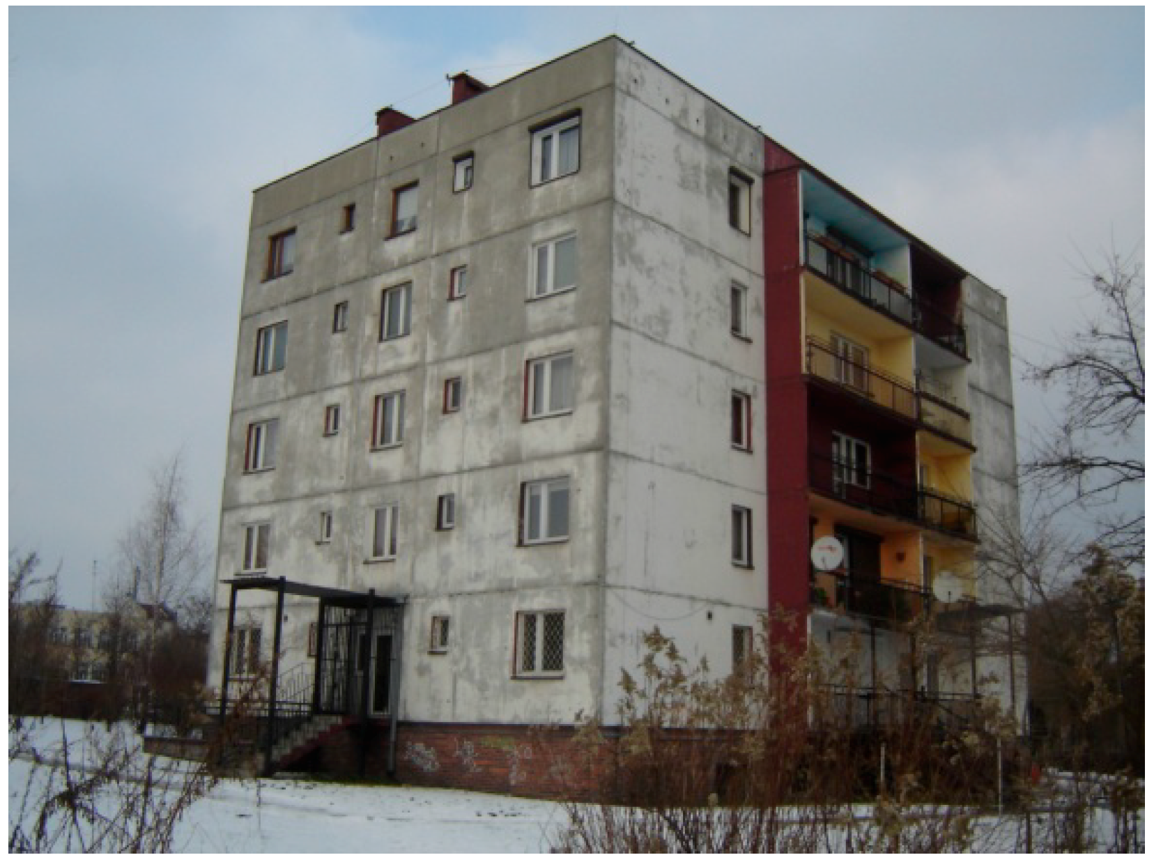
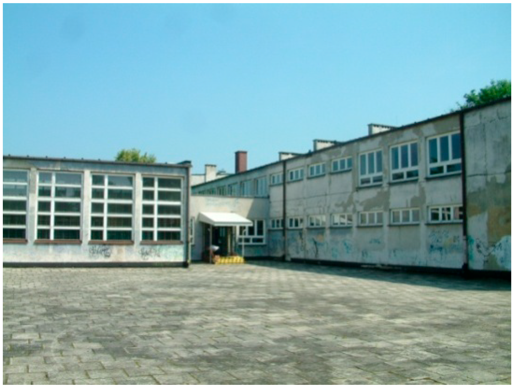
2.1. Description of the Buildings

The first building is a five-story multifamily dwelling house with a total volume of 4318 m³ and a heated area of 1350 m². The building was built in the 1980s (Figure 1). There are four flats on each story (Figure 3a). Gravity ducts are located in kitchens, bathrooms, and separate toilets (in each case one exhaust grille). There are several types of windows in the building, both relatively new, quite tight PVC windows, as well as wooden windows made several decades ago. None of the windows are equipped with air inlets. There are some cracks in the building external walls and poorly sealed crossing of central heating verticals in flats.

The school building (primary school) selected for testing was built in the 1960s (Figure 2). It is a two-story building, without a basement, the total volume of which is 6428 m³, and the heated area is 1406 m². The building consists of two connected parts: a two-story main building, comprising classrooms, office, toilets, kitchen, and cloakrooms and a one-story gym building. There are two classroom-types in the school: type A with an area of 50.5 m² and type B with an area of 67.7 m² (Figure 3b). A total of 20–30 pupils are taught in the classrooms. All windows and doors have been replaced with new ones (wooden or PVC windows). None of the windows are equipped with air inlets. The windows are equipped with a microventilation system in the window sashes, which is activated by turning the handle of closed window by 90–180°; this location causes the window to unseal a little bit to allow for small airflow. Gravity ducts are located in every room. Rooms with higher ventilation requirements (e.g., classrooms) are equipped with more (4–6) ventilation ducts. Inspection of the ventilation system revealed that a considerable part of the ventilation grille in the building was blocked due to the backflow in the ventilation ducts that occurred frequently and caused thermal discomfort to occupants.

2.2. Measuring Instruments

During diagnostics the following measuring equipment was used:

• Minneapolis Blower Door Model 4 for airtightness test (measuring range of air volume: 19–7200 m³/h with uncertainty of ±4%; uncertainty of pressure difference measurement ±1% of reading value or 0.15 Pa).
• SwemaFlow 233 balometer for measuring the airflow in the ventilation grille (measuring range of the volume flow: 2–65 dm³/s; the accuracy: ±4% for 18–25 °C).
• SENSOTRON PS32 indoor air quality monitor for measuring CO₂ concentration (measuring range: 0–5000 ppm; the accuracy: ±20 ppm).
• APAR for indoor temperature measurement (measuring range: −30–80 °C; the accuracy: ±0.5 °C for 20–30 °C, and this may vary between 0.5 and 1.8 °C in the remaining range).
• Weather station (measuring range of temperature: −40–65 °C with uncertainty ±0.5 °C, measuring range of relative humidity: 0%–100% with uncertainty ±3%, measuring range of solar radiation: 0–1800 W/m² with uncertainty ±5%, measuring range of wind speed: 1–80 m/s with uncertainty: ±1 m/s, measuring range of wind direction: 0–360° with uncertainty: ±3°).

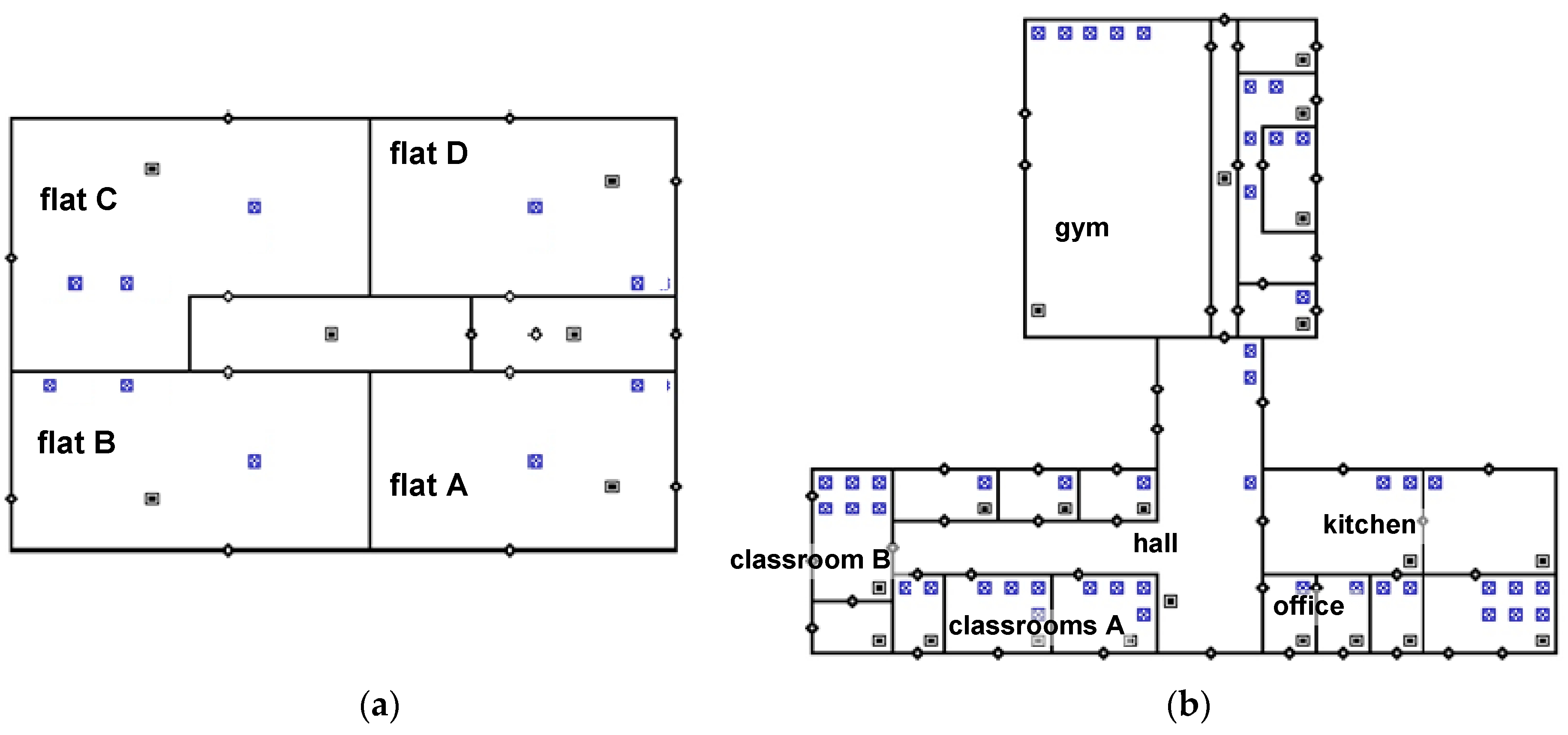
2.3. Airflow Simulation

In order to estimate the airflow throughout the year, simulations were performed. Knowing the characteristics of airtightness and the total length of the leakages in the windows made it possible to build models of the buildings. The simulations were performed using CONTAM software [8] with 1 h time steps. Multizone models of the buildings were built, reproducing all the identified airflow paths: both infiltration through windows and door cracks as well as interzone airflows. The air infiltration coefficients, calculated from airtightness measurements, were used with the assumption of their repeatability in the same type of windows in other zones in the buildings.

In the multifamily building each flat and corridor was modelled as a separate zone, resulting in a total of 30 zones. In the flats, the doors to individual rooms are open most of the day, which allows for considering the flat as one zone. This problem was discussed in more detail by the authors in [10]. The indoor temperature in the zones was based on the measurements performed from 1 February to 30 April 2016 in four selected flats. The air temperature in the flats was nearly 22 °C throughout the measurement period and such an air temperature was assumed in all zones for calculation purposes, with the exception of the staircase where 2 °C lower was assumed. Figure 3a shows the repetitive story of the building modelled in CONTAM.

For the school building 33 calculation zones were defined, connected to each other or to the ambient environment. The model also includes a staircase connecting the ground floor and the upper floor. Figure 3b shows the ground floor reproduced in the CONTAM program. The indoor temperature was identified in the same way as in case of the residential building, i.e., based on measurements. The temperature was recorded for the period from February to March in 10 representative rooms. The air temperature in the zones changed throughout the day and decreased at weekends. Average air temperature values for individual calculation zones of the simulation model were determined. Depending on the zone, the temperature varied between 16 and 24 °C.

The models were calibrated and verified on the basis of the existing measurement data. The climate data for the validation was prepared using meteorological data recorded by the local weather station.

Next, the simulation of airflows for the whole heating season from October to April (5088 h) was performed for reference weather data for southern Poland—site Katowice [57] (mean external temperature during the heating season is 2.7 °C, with minimum temperature of −19 °C, and maximum of 23 °C). The same climate data is used for certificates and audits of buildings.

2.4. Energy Demand

The seasonal energy demand for ventilation was evaluated. The calculations were performed for the hourly air flow rates obtained from the simulations and from the standard. The energy demand for ventilation airflow obtained from the simulation in CONTAM (in kWh/m²) was calculated in Excel from Equation (5) as the sum of the heat demand in all calculation zones and all calculation steps.

$$Q_{V(simul)}={\displaystyle \sum _{j=1}^n{\displaystyle \sum _{k=1}^{5088}\frac{{\dot{V}}_j}{3600·A_j}}}·(t_{i_k}-t_{e_k})·\rho ·c_p,$$

(5)

where:

• t_i—indoor temperature in the j-zone, °C,
• $t_{e_k}$—outdoor temperature in the each time step, °C,
• A_j—heated area j-zone, m²,
• ${\dot{V}}_j$—airflow in each time step for j-zone, m³/h,
• n—number of zones,
• c_p—specific heat of dry air, 1.005 kJ/(kg·K),
• ρ—density of air, 1.204 kg/m³.

The energy demand for ventilation airflow obtained from the standard (in kWh/m²) was calculated from the equation:

$$Q_{V(ST)}={\displaystyle \sum _{k=1}^{5088}\frac{{\dot{V}}_{ST}}{3600·A}}·(t_{i_{mean}}-t_{e_k})·\rho ·c_p,$$

(6)

where:

• $t_{i_{mean}}$—mean indoor temperature in building, °C,
• $t_{e_k}$—outdoor temperature in the each time step, °C,
• A—heated area of building, m²,
• ${\dot{V}}_{ST}$—airflow in the building from the standard [56], m³/h,
• c_p—specific heat of dry air, 1.005 kJ/(kg·K),
• ρ—density of air, 1.204 kg/m³.

3. Results

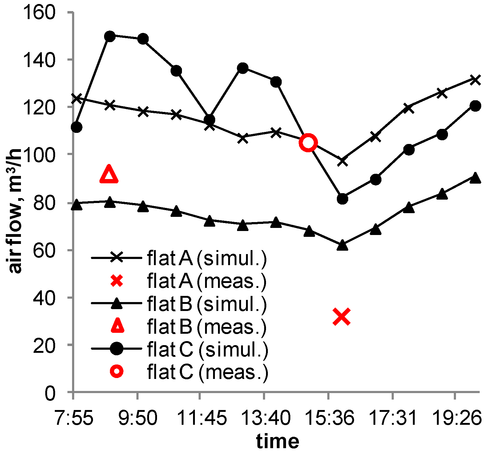
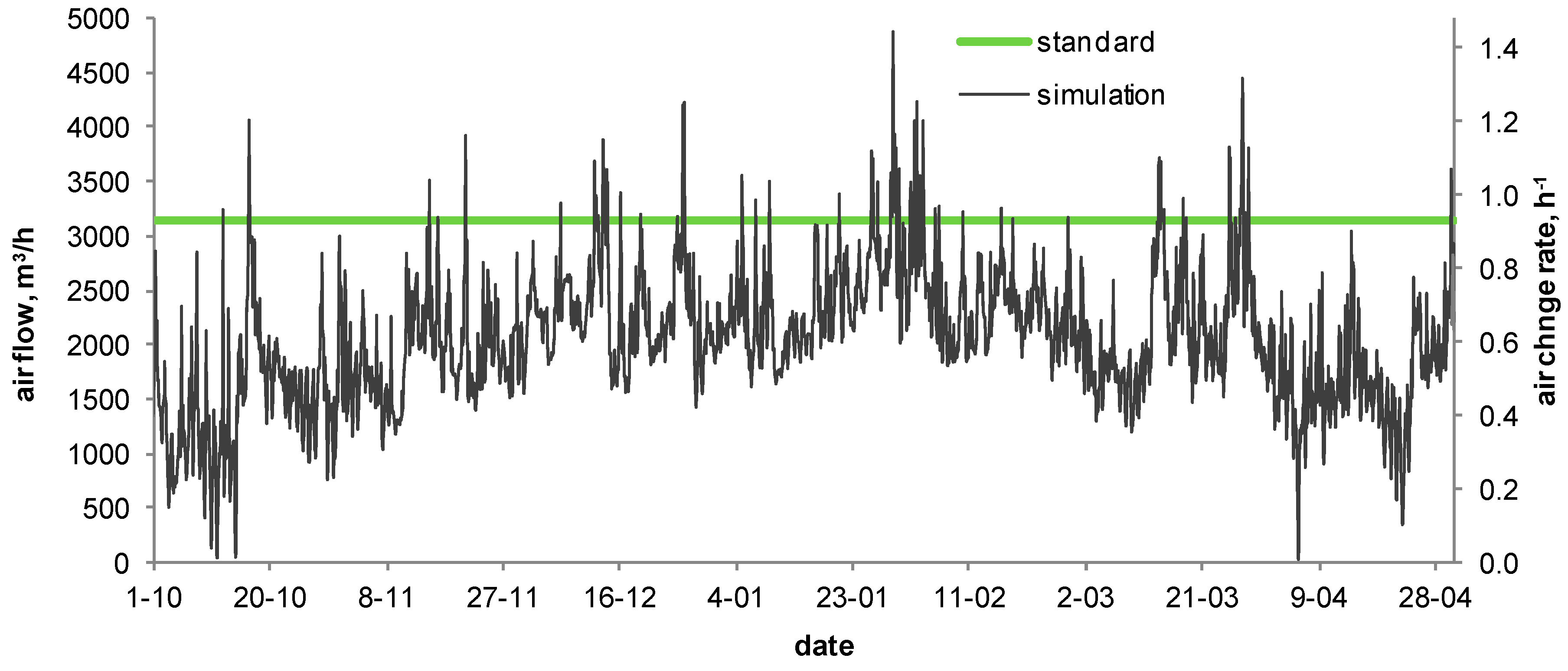
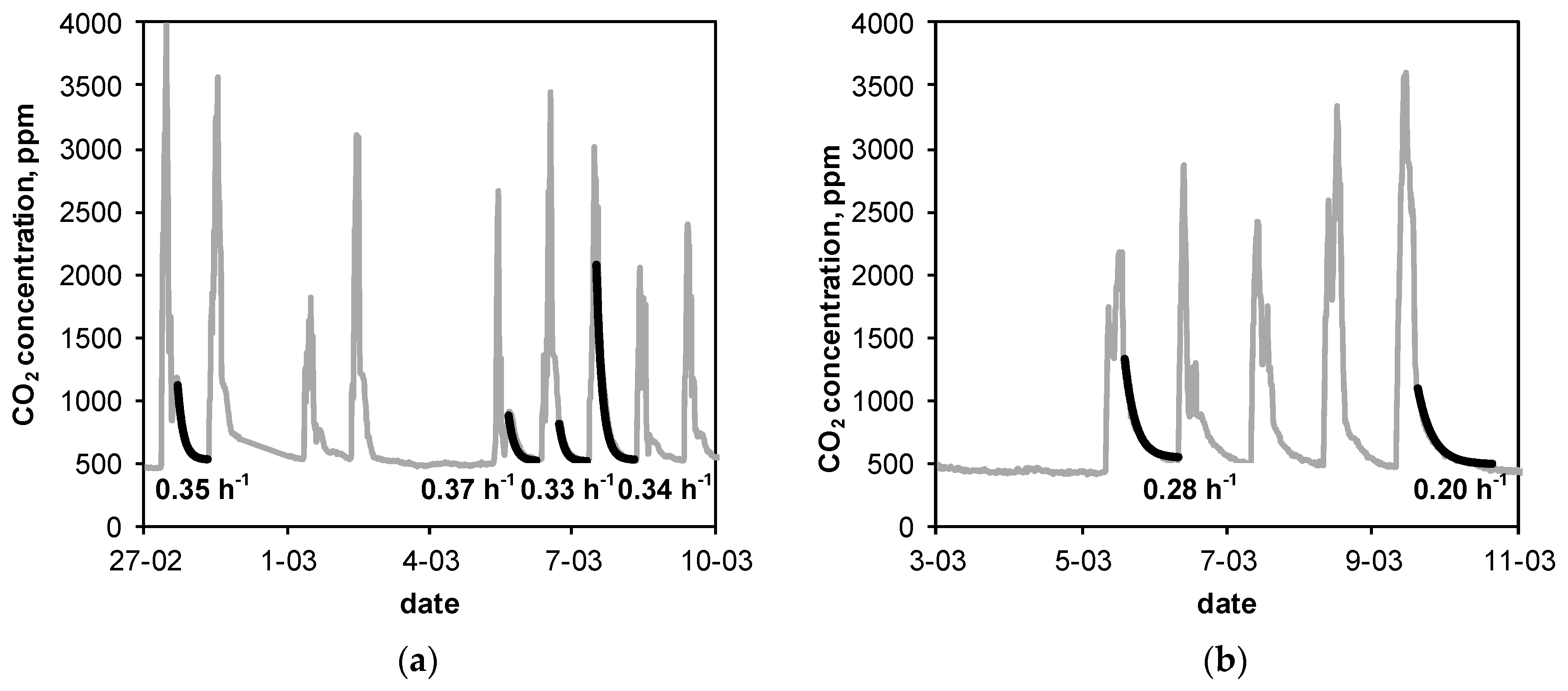
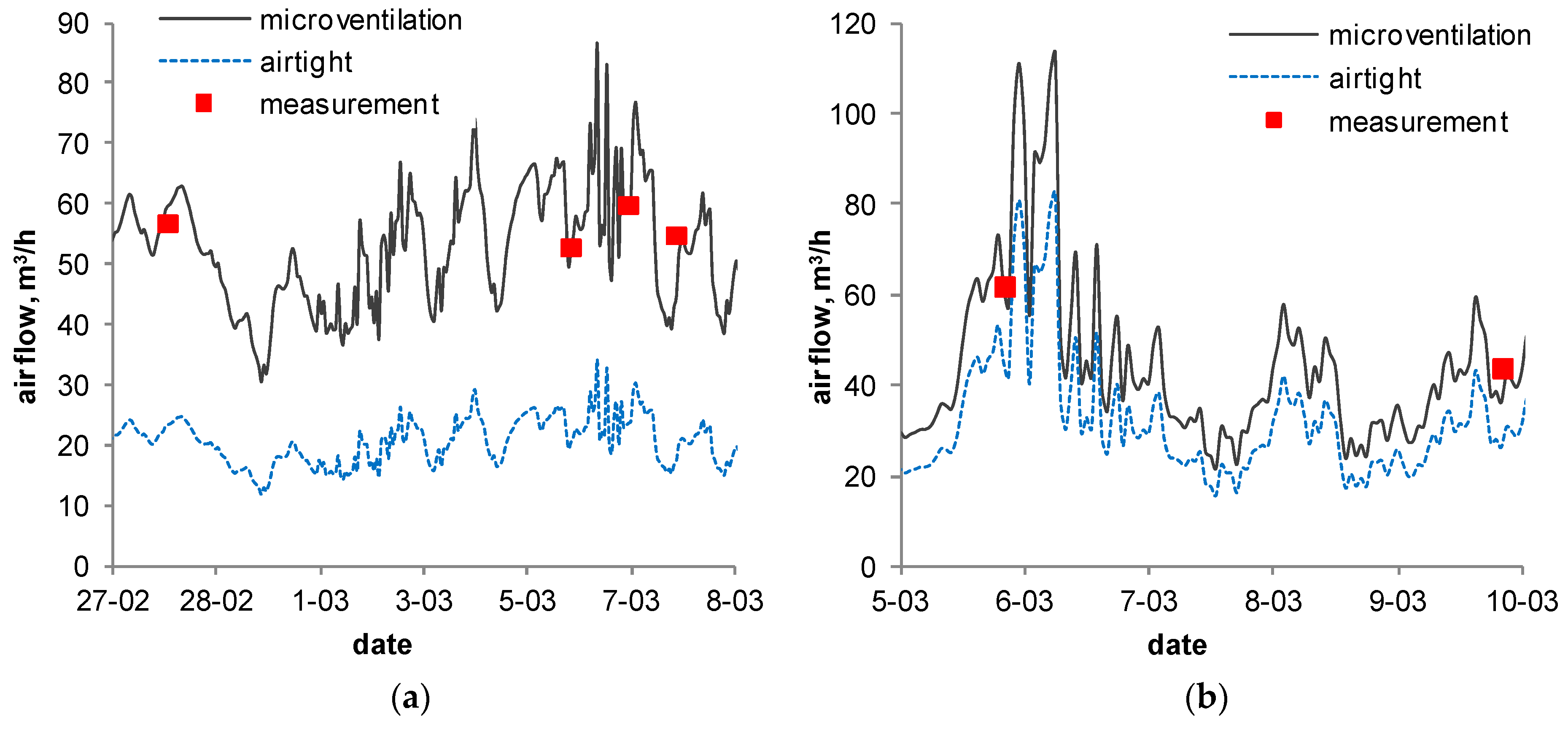
3.1. The Multifamily Building

The measurements concerned three flats: two on the 2nd story (A and B) and one on the 5th story (C) (see Figure 3a). The selection was random and dependent on the consent of on the part of the tenants to carry out the measurements. The measurements of airflow in the ventilation grilles were made in February. All windows were closed during measurement. The outside temperature was around 3.5 °C, the day was relatively windy, the wind speed was around 2.5 m/s. The results are shown in

Table 1. Measurement results of tightness and ventilation airflows in the multifamily building.

Flat	Window Type	Airtightness Test				Measurement in Air Outlets
		C, m3/(h·Pa0.67)	${\dot{\mathit{V}}}_{50},$ m3/h	n50, h−1	Airtightness Factor a, m3/(m·h·Pa0.67)	Kitchen/Bathroom/Toilet, m3/h	Sum of Airflow 1 (Required Airflow 2), m3/h	Air Change Rate, h−1
A (2nd story)	old (wood)	30.6	415	3.3	1.16	32/0	32 (120)	0.25
B (2nd story)	new (PVC)	17.5	232	1.5	0.54	30/32/30	92 (150)	0.61
C (5th story)	old/new(wood/PVC)	50.8	715	3.8	1.37	40/30/35	105 (150)	0.57

¹ The sum of ventilation airflows in all grilles of the flat. ² According to the Polish standard [56].

.

During the airtightness test, it was necessary to seal some components of the electrical installation, as well as culverts of the central heating verticals and culverts of the gas installation. Grille outlets were also sealed. Since the bathrooms were interior rooms, without windows and external walls, they were isolated by sealing the door for the period of measurements. Consequently, leakiness problems in these rooms were circumvented. The device was located in the entrance doors of the flats (Figure 4).

The results of pressurization tests are presented in Table 1 (average underpressure and overpressure values in the zone). In cases where the value of exponent n was not equal to 0.67, the approximation of the curve to 0.67 was performed by looking for a corrected C-factor by the least squares method. Having identified the length of the window cracks the airtightness factors a was also calculated (Table 1). These factors were necessary to carry out the next step of numerical simulations.

The removed airflow did not reach the value resulting from the PN-83/B-03430/Az3 standard [56] in any of the surveyed flats. In flat A (with one ventilation grille in the kitchen and one in the bathroom) the ventilating airflow should have been 120 m³/h, while the measured value was four times lower. Obstruction was detected in one of the grilles, the measurement showed no flow. Such a situation led to a significant reduction of the ventilation flow in the whole apartment. In other dwellings under consideration equipped with additional toilets, the normative air exchange should be no less than 150 m³/h. In dwellings B and C, the measured exhaust airflows were 92 and 105 m³/h, respectively, so they did not differ from the standards as much as in flat A. It can also be seen that despite the shorter gravity ducts on the highest floor (flat C), the measured ventilation airflows in individual grilles are at a similar level as in the flats on the first floor. For some grilles even a bit higher. The stack effect is not the only important factor, as the number of supply openings in this case the tightness of the windows plays a major role. Flat C has the largest flow coefficient C. The values derived from the quoted standard are used in the calculations of energy consumption for heating (e.g., according to the PN-EN ISO 52016-1:2017-09 standard [58]). The real measured values of airflows represent between 27% and 70% of the standard values. Therefore, the real heat demand will be significantly lower than the one that has been calculated according to the standards.

The measurements also indicate the high level of airtightness of the flats with new PVC windows. The value of n₅₀ does not exceed 2 h⁻¹ (Table 1). As already mentioned, the highest airtightness index was recorded in flat C as it was one of the flats where windows had been replaced with new ones. However, this flat has a relatively large length of window cracks compared to the other flats tested in this building and the largest surface of the external walls of all tested flats. Flat A is only equipped with old leaky windows; however, the length of windows is 11 m less, hence the lower airtightness index. All flats equipped with older windows or mixed windows proved to be of average tightness (values of n₅₀ are in the range of 2–5 h⁻¹ according to the PN-EN 12831:2006 standard [49]). The exponents n of tightness characteristics differed only slightly from the preferred value of 0.67, except for the flat C. This may indicate that there are still other uncontrolled airflow paths that could not be located during the tests.

Figure 5 presents the variation of simulated air ventilation on the day of measurements in the three analyzed flats. A fair compatibility of the measurement results of the airflows exhausted from two flats with calculated air ventilation can be noted. Differences do not exceed 12% for flats B and C. For flat A, the large (two-times) difference may result from substantial contamination to the ventilation grille, so that the airflow was largely through the flat’s door to the staircase, which is not included in the measurement. The simulation model assumed that all ventilation grilles in the building were unobstructed.

The results obtained with the use of numerical calculations are sufficiently close to those obtained by measurements. The presented model is characterized by sufficient accuracy and can be used for airflow calculations of the building during the whole heating season. Figure 6 shows the variation of air infiltration from October to April (with 1 h time step) for the whole building.

According to the standard [56], the ventilation airflow for the whole building should be 3140 m³/h. The maximum calculated airflow in the building was 4884 m³/h. This is 150% of the standard value. However, during the heating season, the value of the airflow was lower than the standard value. For over 70% of the time, the calculated value is from 40% to 80% of the standard value and the mean air volume in the heating season is only 2034 m³/h.

The seasonal heat demand for ventilation is presented in

Table 2. Seasonal airflow and heat demand for infiltration.

Building	Mean Seasonal Airflow, m3/h			Heat Demand, kWh/m2
	From Simulation	From the Standard	Difference	Infiltration from Simulation	Infiltration from the Standard	Difference
Residential	2034	3140	−35%	52.3	75.3	−31%
School	987	1835	−46%	23.1	38.5	−40%

. For the calculation of heat demand with the airflow conforming to the standard the assumed indoor temperature was 21.6 °C (weighted average temperature in the building, determined from the measurement, see Section 2.3). Calculation of the value of the airflow based on the standard causes an overestimation of heat demand for its heating of over 30%.

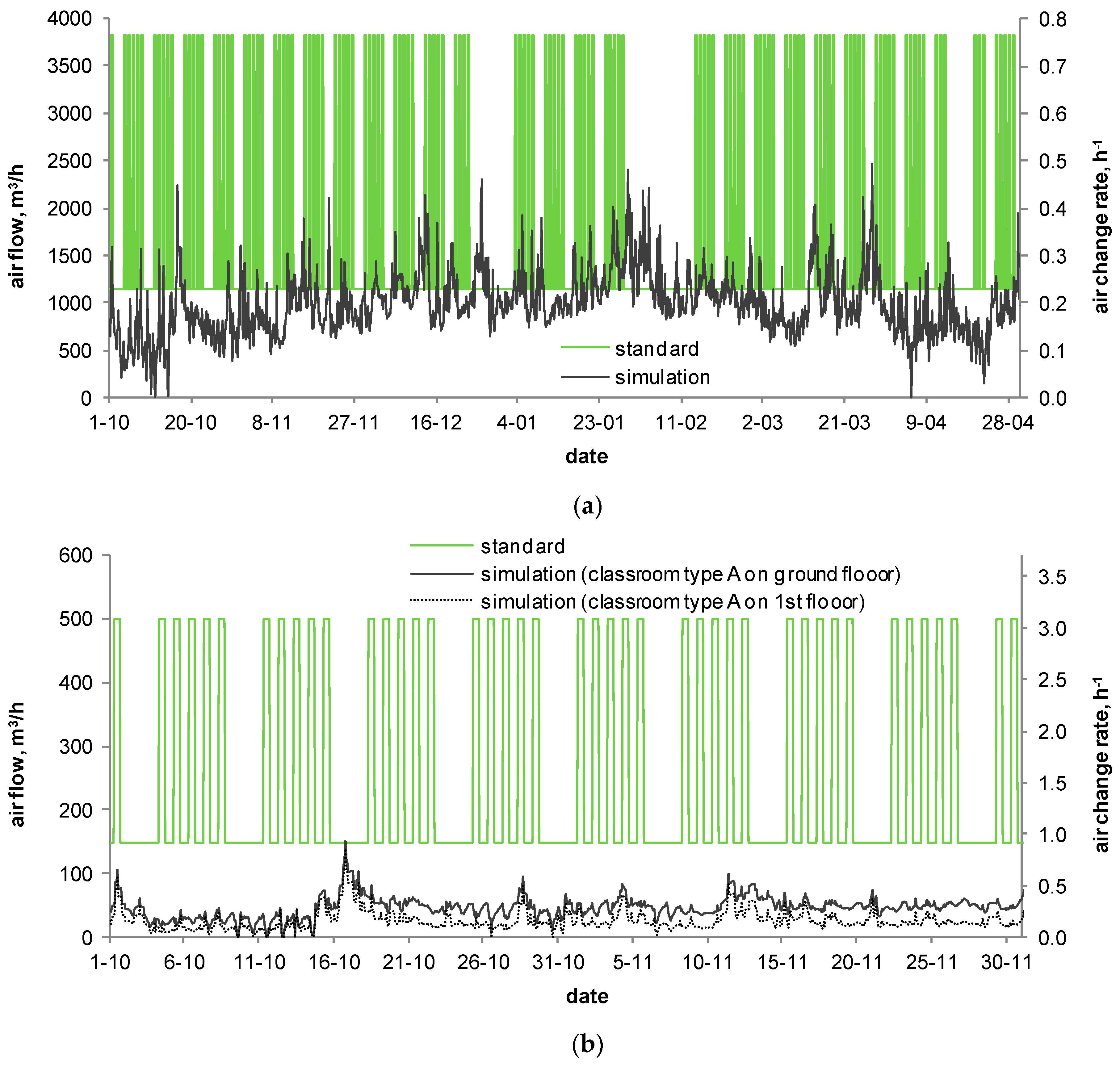
3.2. The School Building

Air exchange in the classrooms should be at least 2 h⁻¹ [49]. However, the hygienic flow of ventilation air should be 20 m³/h person. The contradiction in these requirements is obvious, especially if they are compared with the results of measurements. Uncertainty of measurement also results from the frequent airing of classrooms during breaks, which significantly improves indoor air quality, but increases heat demand.

Carbon dioxide concentration loggers were located in three classrooms for 2 weeks (February/March). The concentration was measured with 5 min time steps. Recorded CO₂ concentration allowed to determine the number of air exchanges using the concentration decay method of carbon dioxide generated by metabolism in two classrooms. During the measurement period there were about 30 occupants in the classrooms. Maximum CO₂ concentration in the day ranged from 4000 to 5000 ppm (Figure 7), but the classrooms were intensely ventilated by opening the window during breaks or after lessons therefore, such a high level is short-lived. However, high level of CO₂ concentration indicates insufficient ventilation in classrooms with closed windows. Poor air quality recorded in classrooms is not an isolated problem, as other researchers point out. For example, Ma et al. [59] showed that the average daily CO₂ concentration in classrooms in China was 1510–3863 ppm, which is far higher than the recommended value of 1000 ppm. In other studies, the maximum CO₂ concentration in naturally ventilated classrooms is generally 4–6 times higher than the reference value [60,61,62,63,64,65].

A free decay of CO₂ concentration above a value of at least twice the background level was recorded five times in the classroom on the ground floor and two times in the classroom on the upper floor (Figure 7). Using Equation (1), the value of the air change rate was calculated.

Airtightness measurements were performed in two classrooms equipped with different types of windows. It was necessary to seal some of the electrical installation components and the culverts of the central heating elements for measurement purposes. The ventilation grilles were also covered. The blower door device was mounted in the door of the classrooms. Measurements were performed with closed windows and at microventilation positions.

Diagnostics of the ventilation system show that, in the case of the analyzed school, ventilation is insufficient. Although the ventilation ducts are unobstructed and their number is large (especially in classrooms), the high level of airtightness of the windows limits the inflow of fresh air. The downdraught resulted in the need to cover a large part of the exhaust grilles, especially on the upper floor of the building. Unfortunately, the ventilation airflow in the classrooms is small and significantly differs from the hygienic requirements (20 m³/h per person). CO₂ concentration at the end of the lesson decayed to the background level in about 10–12 h, and the value of the air change rate ranged from 0.20 to 0.37 h⁻¹ (Figure 7). The air exchange in the hall on the ground floor was larger than that on the upper floor, but insufficient for the requirements. Despite the greater ventilation, the carbon dioxide concentration in the classroom on the ground floor is larger than classroom on the 1st floor (with the same number of students) due to the smaller cubic capacity of this room.

The air flow rate in the classroom on the ground floor determined by the method of concentration decay ranged from 53 to 89 m³/h, while that required for 25 pupils is 500 m³/h. In the classroom on the 1st floor, the number of exchanges did not exceed 0.3 h⁻¹. Poor ventilation in this room is due to limited length of the ventilation duct and the fact that the ventilation grilles in the room were closed (owing to the frequent downdraught in the ducts) and the air exhaust takes place mainly through ventilation grilles placed in the back of the room (the airflows through leaks in the door between rooms).

Tightness measurements confirm a very high level of airtightness of the building (

Table 3. Air tightness measurement results in the school building (average values for under- and overpressure in the rooms).

Room	Case	C, m3/(h·Pa0.67)	${\dot{\mathit{V}}}_{50},$ m3/h	n50, h−1	Airtightness Factor a, m3/(m·h·Pa0.67)
Classroom with wooden windows	Airtight windows	6.2	81	0.49	0.10
	Windows with microventilation	15.8	224	1.37	0.24
Classroom with PVC windows	Airtight windows	12.0	165	0.77	0.16
	Windows with microventilation	17.2	238	1.12	0.22

). The value of n₅₀ does not exceed 2 h⁻¹ even for the microventilation case. Although the length of the cracks is twice as large as in the previously tested dwellings, the tightness index n₅₀ does not exceed 1 h⁻¹.

Simulations were performed for two window leakage cases resulting from the pressure test—for tight windows and when the microventilation system was used. Figure 8 shows the course of variation for the calculated and measured ventilation airflow (by the CO₂ concentration decay method) for the classroom on the ground floor and on the upper floor. In the graph, the measurement points represent the mean airflow from the period of tracer gas concentration decay (see Figure 7).

Unsealing of windows has a very significant effect on the air infiltration to the rooms. During the period of February and March, the airflow increased by 6–32 m³/h on the upper floor and by 19–61 m³/h on the lower floor when the windows were unsealed—that is 45% in the first and 165% in the second case.

There is close agreement between measurements and the simulation results for the microventilation case. The average difference in measuring periods did not exceed 10%; therefore, further research was performed for the microventilation case. This model can be considered sufficiently accurate and can be used for calculating the ventilation airflow throughout the whole heating season. Figure 9 shows the variation of the infiltration airflow (with 1 h time step) for the entire building.

The infiltration airflow varies greatly during the heating season—from near zero to 2468 m³/h. The mean value of ventilation air is 987 m³/h in this period. Assuming 20 m³/h per person as according to the standard [56], this airflow should amount to 3820 m³/h (191 persons in the school). As demonstrated by simulations, such a flow of ventilation air never occurs. Calculated by numerical simulation, the maximum ventilation airflow is 65% of the maximum required standard value. For only 20% of the time, the ventilation airflow exceeds half of the required value. The case of the building with unsealed windows is considered, which is more useful when considering air infiltration. As it can be seen in Figure 9, the higher values of the infiltration airflow appear during night hours when the building is not in use. This is due to the decrease in ambient temperature and thus the increase in the difference between indoor and outdoor temperature. Inability to control ventilation system causes an unnecessary increase in demand for heat in the periods when the demand could be reduced. Analyzing the results for a single classroom, it can be observed that the airflow for the whole heating season is far below the required value (Figure 9b). The maximum value obtained in classroom A is 150 m³/h and the mean in the season is 52 m³/h. On average, during the use of the classroom, the calculated value is only 10% of the required value. Such a small flow of ventilation air is seen in the ground-floor room, in which there are four ventilation grilles. In the same classroom on the upper floor, airflow (due to the smaller stack effect) is even smaller (on average 48%), although there are more ventilation grilles.

Assuming the possibility of reducing the ventilation flow during the night (from 19:00 to 5:00) every day and at weekends and holidays by up to 30% of the required value, the standard seasonal airflow for the entire building should be 1835 m³/h, while for the classroom 240 m³/h. The calculated average airflow during the heating season is 54% of the standard value, which is a huge difference in heat demand in both cases. The seasonal heat demand for ventilation is presented in Table 2. For the calculation of heat demand according to standard airflow, the assumed indoor temperature was 20.6 °C. The heat demand calculated from the ventilation airflows obtained from the simulation represents 60% of the calculated heat demand, considering the standard airflow values.

In practice, classrooms are more or less regularly ventilated during breaks, for example by opening windows (which is not included in this study). This will significantly increase the average daily and seasonal airflow, and thus the heat consumption necessary for the heating of the ventilation air. Such analyses can be found in the previous authors’ papers [5,21].

4. Conclusions

The article presented various methods (measurement and computational) of natural ventilation assessment. Due to use of the buildings and the limited access to them (private flats), not all the methods were tested in both of the selected buildings. The air change rate calculated on the basis of the measurement of airflow in the grilles or by the concentration decay method is not always a measure of the fresh airflow, because there are also interzone flows and the air used may flow into the room, e.g., from the staircase. The airflow between the flat and the staircase and in the staircase itself with natural chimney draft can sometimes be large. In this situation, the measurement gives inflated air change rate. Moreover, oftentimes simulation calculations of airflow may be burdened with error, if an inaccurate model of a building is built or incorrect simulation data are introduced, e.g., meteorological data or air infiltration coefficients for individual flow paths.

The observations above must be considered when analyzing the results of the measured air removal only in the ventilation grids. In addition, the results of measurements are for instantaneous values, which are subject to e.g., a temporary influence of adverse wind or the opening of the entrance door to the building.

The conducted research allowed the elaboration of the following main conclusions:

• airtightness of the tested buildings is within the ranges specified in the standards; a high level of airtightness of rooms with new tight windows was indicated; the value of n₅₀ does not exceed 2 h⁻¹,
• many uncontrolled leakages, which impede measurements and increase their uncertainty, exist in old buildings; uncertainty as to the results may also result from the fact that the measurements were performed in random buildings, one school and one multifamily building,
• ventilation airflow, measured directly in the exhaust grille of the multifamily house, is small and substantially deviates from the Polish standard (half of the one on average); however, the airflow was measured only in the exhaust grilles, without considering the airflow through the flat doors to the building staircase; the flats are irregularly ventilated by opening the window, which increases the average daily and seasonal airflow, and thus the heat demand for the heating of the ventilation air.
• the measured ventilating airflow in the school building is abnormally low, on average in the heating season almost twice as low as the required value; the simulations show that the use of window microventilation function increases the infiltration airflow to the building from 0.5 to 1.5 times, depending on the room; calculation of the heat demand for ventilation based on the standard value of the airflow will lead to a considerable overestimation of this value in relation to the real requirements (up to 40%).

The performed diagnostics allowed for the detection of problems in the operation of ventilation systems and the development of recommendations for their improvement, as follows:

• checking and cleaning the ventilation grilles in all rooms and checking if there is any obstruction in the ventilation ducts,
• use of microventilation function in windows or the installation of automatically controlled air diffusers in windows or outside walls,
• regular ventilation of the rooms by opening the window,
• installation of a chimney cowl, which should eliminate the backflows, especially in the school building, where this phenomenon had led to the complete closure of some ventilation grids.

In case of the school building, ventilation should be configured with appropriate mechanical ventilation devices in order to secure its the proper operation. Therefore, one of these three systems (in order of investment costs) is proposed [5,21]: exhaust ventilation system (e.g., roof fans) with constant airflow, interchangeable with natural ventilation in periods free from lessons or exhaust ventilation system (roof fans) controlled by carbon dioxide concentration or supply-exhaust ventilation system with a heat recovery system (e.g., compact air handling units in classrooms).

Future Research

This research was focused on the objective evaluation of natural ventilation performance in occupied buildings. The measurements did not consider the effect of natural ventilation on thermal environment and occupants’ comfort. Future research can be also extended to buildings subjected to thermomodernization in which natural ventilation was improved, e.g., by application of trickle window vents.

References

1. Moran, P.; Goggins, J.; Hajdukiewicz, M. Super-insulate or use renewable technology? Life cycle cost, energy and global warming potential analysis of nearly zero energy buildings (NZEB) in a temperate oceanic climate. Energy Build. 2017, 139, 590–607. [Google Scholar] [CrossRef]
2. Liu, L.; Rohdin, P.; Moshfegh, B. LCC assessments and environmental impacts on the energy renovation of a multi-family building from the 1890s. Energy Build. 2016, 133, 823–833. [Google Scholar] [CrossRef]
3. Matzarakis, A.; Balafoutis, C. Heating degree-days over Greece as an index of energy consumption. Int. J. Climatol. 2004, 24, 1817–1828. [Google Scholar] [CrossRef]
4. Liddament, M.W.A. Guide to Energy Efficient Ventilation, Air Infiltration and Ventilation Centre; University of Warwick: Coventry, UK, 1996. [Google Scholar]
5. Ferdyn-Grygierek, J. Impact of ventilation systems on indoor air quality and annual energy consumption in school buildings. In Proceedings of the 25th AIVC Conference Ventilation and retrofitting, Prague, Czech Republic, 15–17 September 2004; pp. 255–260. [Google Scholar]
6. Maile, T.; Bazjanac, V.; Fischer, M. A method to compare simulated and measured data to assess building energy performance. Build. Environ. 2012, 56, 241–251. [Google Scholar] [CrossRef]
7. Zhaia, Z.; El Mankibib, M.; Zoubir, A. Review of natural ventilation models. Energy Procedia 2015, 78, 2700–2705. [Google Scholar] [CrossRef]
8. Walton, W.G.N.; Dols, S. CONTAM 2.4 User Guide and Program Documentation; National Institute of Standards and Technology: Gaithersburg, MD, USA, 2005.
9. Li, Z.R.; Ai, Z.T.; Wang, W.J.; Xu, Z.R.; Gao, X.Z.; Wang, H.S. Evaluation of airflow pattern in wind-driven naturally ventilated atrium buildings: Measurement and simulation. Build. Serv. Eng. Res. Technol. 2014, 35, 139–154. [Google Scholar] [CrossRef]
10. Baranowski, A.; Ferdyn-Grygierek, J. Effect of calculation zoning on numerical modelling of ventilation airflows. Build. Simul. 2015, 873–879. [Google Scholar] [CrossRef]
11. Stavridou, A.D.; Prinos, P.E. Natural ventilation of buildings due to buoyancy assisted by wind: Investigating cross ventilation with computational and laboratory simulation. Build. Environ. 2013, 6, 104–119. [Google Scholar] [CrossRef]
12. Freire, R.Z.; Abadie, M.O.; Mendes, N. On the improvement of natural ventilation models. Energy Build. 2013, 62, 222–229. [Google Scholar] [CrossRef]
13. Zhou, J.; Ye, C.; Hu, Y.; Hamida, H. Development of a model for single-sided, wind-driven natural ventilation in buildings. Build. Serv. Eng. Res. Technol. 2017, 38, 381–399. [Google Scholar] [CrossRef]
14. Martins, N.R.; Carrilho da Graça, G. Validation of numerical simulation tools for wind-driven natural ventilation design. Build. Simul. 2016, 9, 75–87. [Google Scholar] [CrossRef]
15. Hyun, S.-H.; Park, C.-S.; Augenbroe, G. Analysis of uncertainty in natural ventilation redictions of high-rise apartment buildings. Build. Serv. Eng. Res. Technol. 2008, 29, 311–326. [Google Scholar] [CrossRef]
16. Dols, W.S.; Emmerich, S.J.; Polidoro, B.J. Using coupled energy, airflow and indoor air quality software (TRNSYS/CONTAM) to evaluate building ventilation strategies. Build. Serv. Eng. Res. Technol. 2016, 37, 163–175. [Google Scholar] [CrossRef] [PubMed]
17. Aparicio-Fernández, C.; Vivancos, J.-L.; Cosar-Jorda, P.; Buswell, R.A. Energy modelling and calibration of building simulations: A case study of a domestic building with natural ventilation. Energies 2019, 12, 3360. [Google Scholar] [CrossRef]
18. Baranowski, A.; Ferdyn-Grygierek, J. Heat demand and air exchange in a multifamily building—Simulation with elements of validation. Build. Serv. Eng. Res. Technol. 2009, 30, 227–240. [Google Scholar] [CrossRef]
19. Omrani, S.; Garcia-Hansen, V.; Capra, B.; Drogemuller, R. Natural ventilation in multi-storey buildings: Design process and review of evaluation tools. Build. Environ. 2017, 116, 182–194. [Google Scholar] [CrossRef]
20. Ben-David, T.; Waring, M.S. Impact of natural versus mechanical ventilation on simulated indoor air quality and energy consumption in offices in fourteen U.S. cities. Build. Environ. 2016, 104, 320–336. [Google Scholar] [CrossRef]
21. Popiołek, Z.; Ferdyn-Grygierek, J. Efficiency of heating and ventilation in school buildings before and after retrofitting. In Proceedings of the 3rd International Seminar Healthy Buildings, Sofia, Bulgaria, 18 November 2005; pp. 67–76. [Google Scholar]
22. Wong, N.H.; Wang, L.; Aida, N.C.; Anupama, R.P.; Wei, X. Effects of double glazed facade on energy consumption, thermal comfort and condensation for a typical office building in Singapore. Energy Build. 2005, 37, 563–572. [Google Scholar]
23. Mateus, N.M.; Simões, G.N.; Lúcio, C.; Carrilho da Graca, G. Comparison of measured and simulated performance of natural displacement ventilation systems for classrooms. Energy Build. 2016, 133, 185–196. [Google Scholar] [CrossRef]
24. Mumovic, D.; Davies, M.; Ridley, I.; Altamirano-Medina, H. A methodology for post-occupancy evaluation of ventilation rates in schools. Build. Serv. Eng. Res. Technol. 2009, 30, 143–152. [Google Scholar] [CrossRef]
25. Kim, J.; Dear, R. Thermal comfort expectations and adaptive behavioural characteristics of primary and secondary school students. Build. Environ. 2018, 127, 13–22. [Google Scholar] [CrossRef]
26. ANSI/ASHRAE Standard 62.1-2019 Ventilation for Acceptable Indoor Air Quality; American Society of Heating, Refrigerating and Air Conditioning Engineers: Atlanta, GA, USA, 2019.
27. EU Standard EN 16798-1:2019. Energy Performance of Buildings—Ventilation for Buildings—Part 1: Indoor Environmental Input Parameters for Design and Assessment of Energy Performance of Buildings Addressing Indoor Air Quality, Thermal Environment, Lighting and Acoustics—Module M1-6; European Committee for Standardization: Brussels, Belgium, 2019. [Google Scholar]
28. Persily, A. Challenges in developing ventilation and indoor air quality standards: The story of ASHRAE Standard 62. Build. Environ. 2015, 91, 61–69. [Google Scholar] [CrossRef] [PubMed]
29. Ferdyn-Grygierek, J.; Blaszczok, M. Energy consumption in school buildings before and after thermomodernization. In Proceedings of the 2nd International Conference on Advanced Construction, Kaunas, Lithuania, 11–12 November 2010; pp. 227–235. [Google Scholar]
30. Seduikyte, L.; Paukstys, V.; Sadauskiene, J.; Dauksys, M.; Pupeikis, D.; Ivanauskas, E. Evaluation of energy performance and environmental conditions in Lithuanian schools. In Proceedings of the 12th International Multidisciplinary Scientific GeoConference of Modern Management of Mine Producing, Geology and Environmental Protection (SGEM 2012), Albena, Bulgaria, 17–23 June 2012; Volume 4, pp. 979–986. [Google Scholar]
31. Stabile, L.; Massimo, A.; Canale, L.; Russi, A.; Andrade, A.; Dell’Isola, M. The effect of ventilation strategies on indoor air quality and energy consumptions in classrooms. Buildings 2019, 9, 110. [Google Scholar] [CrossRef]
32. Stabile, L.; Buonanno, G.; Frattolillo, A.; Dell’Isola, M. The effect of the ventilation retrofit in a school on CO2, airborne particles, and energy consumptions. Build. Environ. 2019, 156, 1–11. [Google Scholar] [CrossRef]
33. Dias Pereira, L.; Bispo Lamas, F.; Gameiro da Silva, M. Improving energy use in schools: From IEQ towards energy-efficient planning—Method and in-field application to two case studies. Energy Effic. 2019, 12, 1253–1277. [Google Scholar] [CrossRef]
34. Ali, H.; Hashlamun, R. Envelope retrofitting strategies for public school buildings in Jordan. J. Build. Eng. 2019, 25, 100819. [Google Scholar] [CrossRef]
35. Ascione, F.; Bianco, N.; De Masi, R.F.; Mauro, G.M.; Vanoli, G.P. Energy retrofit of educational buildings: Transient energy simulations, model calibration and multi-objective optimization towards nearly zero-energy performance. Energy Build. 2017, 144, 303–319. [Google Scholar] [CrossRef]
36. Meiss, A.; Padilla-Marcos, M.A.; Feijó-Muñoz, J. Methodology applied to the evaluation of natural ventilation in residential building retrofits: A case study. Energies 2017, 10, 456. [Google Scholar] [CrossRef]
37. Heracleous, C.; Michael, A. Experimental assessment of the impact of natural ventilation on indoor air quality and thermal comfort conditions of educational buildings in the Eastern Mediterranean region during the heating period. J. Build. Eng. 2019, 26, 100917. [Google Scholar] [CrossRef]
38. Peel, M.B.; Finlayson, B.L.; McMahon, T.A. Updated world map of the Köppen-Geiger climate classification. Hydrol. Earth Syst. Sci. 2007, 11, 633–1644. [Google Scholar] [CrossRef]
39. Cohen, R.; Standeven, B.; Bordass, B.; Leaman, A. Assessing building performance in Use 1: The Probe process. Build. Res. Inf. 2001, 29, 85–102. [Google Scholar] [CrossRef]
40. EU Standard EN 15239:2007 Ventilation of Buildings—Energy Performance of Buildings—Guidelines for Inspection of Ventilation Systems; European Committee for Standardization: Brussels, Belgium, 2007.
41. Blaszczok, M.; Król, M.; Hurnik, M. On-site diagnostics of the mechanical ventilation in office buildings. Archit. Civ. Eng. Environ. 2017, 10, 145–156. [Google Scholar] [CrossRef] [Green Version]
42. Larsen, T.S. Natural Ventilation Driven by Wind and Temperature Difference. Ph.D. Thesis, Aalborg University, Aalborg, Denmark, 2006. [Google Scholar]
43. Charlesworth, P.S. Air Exchange Rate and Airtightness Measurement Techniques—An Applications Guide; Air Infiltration and Ventilation Centre: Coventry, UK, 1988. [Google Scholar]
44. Awbi, H.B. Ventilation of Buildings; Spon Press Taylor & Francis Group: London, UK; New York, NY, USA, 2003. [Google Scholar]
45. EU Standard EN 15242:2007 Ventilation for Buildings—Calculation Methods for the Determination of Air Flow Rates in Buildings Including Infiltration; European Committee for Standardization: Brussels, Belgium, 2007.
46. ISO 12569:2017 Thermal Performance of Buildings and Materials—Determination of Specific Airflow Rate in Buildings—Tracer Gas Dilution Method; International Organization for Standardization: Geneva, Switzerland, 2017.
47. Etheridge, D. Natural Ventilation of Buildings: Theory, Measurement and Design; John Wiley & Sons, Ltd.: Chichester, UK, 2012. [Google Scholar]
48. EU Standard EN 13829: 2001 Thermal Performance of Buildings—Determination of Air Permeability of Buildings: Fan Pressurization Method; European Committee for Standardization: Brussels, Belgium, 2001.
49. Polish Standard PN-EN 12831: 2006 Heating Systems in Buildings—Method for Calculation of the Design Heat Load; Polish Committee for Standardization: Warsaw, Poland, 2006. (In Polish)
50. Feustel, H.E.; Smith, B. (Eds.) COMIS 3.0 User Guide; Lawrence Berkeley Laboratory: Berkeley, CA, USA, 1997.
51. ESRU Manual U02/1. The ESP-r System for Building Energy Simulation, User Guide Version 10 Series; University of Strathclyde. Energy Systems Research Unit: Glasgow, Scotland, 2002. [Google Scholar]
52. Klein, S.A.; Beckman, W.A.; Mitchell, J.W.; Duffie, J.A.; Duffie, N.A.; Freeman, T.L.; Mitchell, J.C. TRNSYS 17 A Transient System Simulation Program; Solar Energy Laboratory, Ed.; University of Wisconsin: Madison, WI, USA, 2010. [Google Scholar]
53. IDA-Indoor Climate and Energy 4.0, Manual Version: 4.0; EQUA Simulation AB: Solna, Sweden, 2009.
54. Guo, H.; Aviv, D.; Loyola, M.; Teitelbaum, E.; Houchois, N.; Meggers, F. On the understanding of the mean radiant temperature within both the indoor and outdoor environment, a critical review. Renew. Sustain. Energy Rev. 2019, 117, 109207. [Google Scholar] [CrossRef]
55. Blaszczok, M.; Baranowski, A. Thermal improvement in residential buildings in view of the indoor air quality—Case study for polish dwelling. ACEE Archit. Civ. Eng. Environ. 2018, 3, 121–130. [Google Scholar] [CrossRef] [Green Version]
56. Polish Standard PN-83/B-03430/Az3: 2000 Ventilation in Dwellings and Public Utility Buildings; Polish Committee for Standardization: Warsaw, Poland, 2000. (In Polish)
57. Typical Meteorological and Statistical Climatic Data for the Energy Calculation of Buildings. Available online: https://www.gov.pl/web/inwestycje-rozwoj/dane-do-obliczen-energetycznych-budynkow (accessed on 28 October 2019).
58. Polish Standard PN-EN ISO 52016-1:2017-09 Energy Performance of Buildings—Calculation of the Building’s Energy Needs for Heating and Cooling, Internal Temperatures and Heating and Cooling Load; Polish Committee for Standardization: Warsaw, Poland, 2017.
59. Ma, F.; Zhan, C.; Xu, X. Investigation and evaluation of winter indoor air quality of primary schools in severe cold weather areas of China. Energies 2019, 12, 1602. [Google Scholar] [CrossRef] [Green Version]
60. Schibuola, L.; Scarpa, M.; Tambani, C. Natural ventilation level assessment in a school building by CO2 concentration measures. Energy Procedia 2016, 101, 257–264. [Google Scholar] [CrossRef]
61. Fadeyi, M.O.; Alkhaja, K.; Sulayem, M.B.; Abu-Hijleh, B. Evaluation of indoor environmental quality conditions in elementary schools’ classrooms in the United Arab Emirates. Front. Archit. Res. 2014, 3, 166–177. [Google Scholar] [CrossRef] [Green Version]
62. Stabile, L.; Dell’Isola, M.; Russi, A.; Massimo, A.; Buonanno, G. The effect of natural ventilation strategy on indoor air quality in schools. Sci. Total Environ. 2017, 595, 894–902. [Google Scholar] [CrossRef]
63. Pereira, L.D.; Raimondo, D.; Corgnati, S.P.; da Silva, M.G. Assessment of indoor air quality and thermal comfort in Portuguese secondary classrooms: Methodology and results. Build. Environ. 2014, 81, 69–80. [Google Scholar] [CrossRef]
64. De Gennaro, G.; Dambruoso, P.R.; Demarinis Loiotile, A.; Di Gilio, A.; Giungato, P.; Tutino, M.; Marzocca, A.; Mazzone, A.; Palmisani, J.; Porcelli, F. Indoor air quality in schools. Environ. Chem. Lett. 2014, 12, 467–482. [Google Scholar] [CrossRef]
65. Fernández-Agüera, J.; Campano, M.A.; Domínguez-Amarillo, S.; Acosta, I.; Sendra, J.J. CO2 Concentration and occupants’ symptoms in naturally ventilated schools in Mediterranean climate. Buildings 2019, 9, 197. [Google Scholar] [CrossRef] [Green Version]
Figure 1. View of the multifamily building selected for the research.
Energies 12 04556 g001
Figure 2. View of the school building selected for the research.
Energies 12 04556 g002
Figure 3. View of one story for CONTAM models of the multifamily building (a) and the school building (b). Blue symbols indicate ventilation ducts.
Energies 12 04556 g003
Figure 4. Blower door mounted in the entrance door to flat C.
Energies 12 04556 g004
Figure 5. Ventilation air flow in analyzed flats of the multifamily building—simulation versus measurement (part of one day in which the measurements were carried out).
Energies 12 04556 g005
Figure 6. Variation of infiltration air flow in the whole multifamily building throughout the heating season.
Energies 12 04556 g006
Figure 7. Variation of CO2 concentration in classroom type A on the ground floor (a) and classroom type B on the upper floor (b). Free concentration decay is indicated (bold lines). The value on the chart signifies the calculated air change rate.
Energies 12 04556 g007
Figure 8. Ventilation air flow in school building—simulation versus measurement: classroom type A on ground floor (a) and classroom type B on first floor (b).
Energies 12 04556 g008
Figure 9. Variation of infiltration air flow in the whole school building throughout the heating season (a) and in classroom type A on the ground floor during two chosen months (b).
Energies 12 04556 g009