1. Introduction
With the rapid development of the motorization process, environmental problems in the traffic field have become increasingly serious in the past decades, which has brought negative impacts on society and public health [
1]. Many study results show that traffic emissions have become an important constituent of pollution emissions [
2], which have also become significant factors hindering the sustainable development of cities. Scholars have conducted a lot of research on air and noise pollution prevention and management from a vehicle engineering perspective [
3,
4,
5,
6], while less attention has been paid to traffic control and other transport operational aspects when making traffic policy.
As the essential nodes in the road network, intersection connects traffic streams from different directions [
7], while the frequent occurrences of acceleration, deceleration and idling conditions of vehicles at intersections cause severe traffic pollution problems. In fact, the efficiency of the overall road network depends a lot on the signal timing strategy at intersections. Therefore, most research concerns the operating status of intersections which are beneficial for reducing traffic accidents and improving traffic efficiency [
8].
Giving priority to public transport has been widely believed to be an effective way of improving traffic efficiency. As the most common public transit, bus takes the advantages of large capacity, less pollution, and low operating cost, which could make the most use of limited road traffic resources and attract more travelers to choose an eco-friendly travel mode. Adopting bus priority strategy at intersections can effectively improve the travel speed of buses and reduce average capita delay, which is of great significance to improve the service quality and reliability of public transport [
9]. Besides, literature also indicates that bus signal priority can improve road safety and should be a major consideration for road management agencies when implementing traffic policy [
10].
Although bus signal priority takes advantage of improving the utilization rate of traffic resources and reducing average capita delay at intersections, there is a possibility that extreme bus signal priority affects traffic conditions for vehicles in other phases, and even aggravates the burden of the whole intersection, resulting in an extra increase in total emissions of exhaust pollutants.
Therefore, how to guarantee the priority of public vehicles without increasing the delay of other vehicles also in an eco-friendly manner has become a crucial issue, which is supposed to be dealt with in this study.
In this paper, a simulation-based method for evaluating the adaptability of BSP aiming at balancing its efficient and environmental impacts is proposed. The rest of this paper is organized as follows. The second section introduces the research status of bus signal priority strategy from three aspects. In the third section, the paper proposes a methodology for evaluating the bus signal priority. The subsequent section presents a case study and compares the performance of different signal timing schemes under hybrid energy consumption conditions. The final section provides a summary and conclusions of the paper.
2. Literature Review
Bus signal priority strategies could be generally divided into three categories: Passive bus signal priority strategy, active bus signal priority strategy, and real-time bus signal priority strategy. For the first, passive bus signal priority strategy almost depends on historical vehicle operational information to determine a preset priority scheme, which is suitable for stable traffic conditions with large traffic flow. Active bus signal priority strategy provides priority signals for specific vehicles with the coordination of the coil detector. And real-time bus signal priority strategy collects arrival information of buses and other vehicles online, and then develops an algorithm to determine bus priority strategy at a specific signal phase in real time.
2.1. Passive Bus Signal Priority
Research on passive bus signal priority attempts to make appropriate signal timing schemes with different optimization objectives. Most scholars focus on strategy design with an efficiency-related objective. For example, Viegas et al. optimized the signal timing parameters of an intersection with the discontinuous bus lane, results show that, basically, the setting of the bus lane can reduce bus delay and will not increase other vehicles’ delay too much [
11]. Zhang et al. studied the variations of bus delays and other vehicle delays before and after setting pre-signal, and the result points out that pre-signal control can reduce average bus delays effectively but increase average delays of other vehicles [
12]. Skabardonis analyzed different bus signal priority strategies in light of the utilization rates of effective green time, green waveband of trunk road, and the punctuality rates of the buses [
13]. Zyryanov et al. explored the impact of bus signal priority strategy with different traffic volumes, then estimated the running speeds of buses and other vehicles when the traffic volume raised [
14]. Xiong et al. solved the passive bus signal priority optimization model with a particle swarm algorithm, in which minimizing average capita delay and exhaust emission were set as the optimization objectives [
15]. Ye and Ma employed VISSIM to simulate traffic conditions with setting the bus lane in the middle or edge of the road [
16]. Guler et al. proposed a method for bus priority at intersections with a single approach lane, which tried to reduce the bus delay by introducing a pre-signal [
17].
The above studies attempt to give priority to buses by adjusting cycle length and green time. In such cases, it assumes that the arrival time of buses is fixed, and the interval of arrival stays the same. However, in reality, affected by the unstable stop time and dynamic road conditions, the arrival time of buses is more likely to be randomly distributed. In this regard, the feasibility of the proposed methodology is limited to some extent.
2.2. Active Bus Signal Priority
Since the 1970s, scholars started to conduct a series of studies on active bus signal priority strategies. Elia et al. proposed a bus signal priority strategy considering the departure time and departure interval of buses, which reduced bus delays effectively [
18]. While Salter et al. pointed out that, irrational bus signal priority may lead to an increase in other vehicles’ delays [
19]. Dion et al. evaluated the adaptability of single-point active bus signal priority, and proposed a method for guiding how to interrupt the current phase and determine which phase should be next [
20].
As above, previous studies only considered one priority request at a time. He et al. proposed a control strategy considering the priority requests from more than one bus, aiming at reducing average vehicle delay and pedestrian delay [
21]. Based on traffic flow and occupancy status detected by the sensing coil, Ma et al. proposed a monitoring approach for vehicle queuing length at an oversaturated intersection and further demonstrated its rationality [
22]. Zhou et al. developed an active bus signal priority strategy for BRT (bus rapid transit) vehicles with an exclusive BRT lane at a single intersection, in which maximizing benefits of BRT and other road users was regarded as the optimization objective [
23]. Wu et al. analyzed the impacts of green time extension and red time truncation strategies on the delay of buses and other vehicles. It was believed that bus signal priority could reduce the total delay at an intersection effectively [
24].
Studies on active bus signal priority mainly focuse on how to grasp more precise arrival time of buses. Since limited work has been done to evaluate the operating status of other vehicles, how to balance the operating efficiency of buses and other vehicles is still a common concern for future research.
2.3. Real-Time Bus Signal Priority
When it comes to real-time bus signal priority control, scholars are concerned more with the design of the bus lane. Viegas et al. pointed out that intermittent bus lanes could be applied and used the arrival information of buses to determine whether other vehicles can enter the bus lane or not [
25]. Guan et al. comprehensively considered actual traffic conditions, bus passengers‘ behavior of getting on and off the bus and arrival time of the bus, then established a real-time control strategy for a single-point signal control intersection [
26]. Zhang et al. analyzed the implementation effect of bus signal priority in light of social economy, environmental impact, and traffic resource utilization. The results show that the proposed method makes average vehicle delay increase slightly compared with the traditional method, but bus delays and per capita delays fell sharply, proving that bus signal priority performs well while the intersection is not severely congested [
27]. Christofa et al. established a real-time bus signal priority system and conducted a simulation test on a complicated signalized intersection which shows that the system can reduce transit users‘ delay effectively [
28]. Ahmed et al. also presented a real-time bus signal system but it considered bus signal priority, incident detection, and congestion management more comprehensively, aiming at improving the efficiency of the whole traffic network [
29].
Kind of different from the above studies, Zeng et al. emphasized the core component of real-time bus signal priority optimization by using a stochastic mixed-integer nonlinear program as the core computing module, which also considered the randomness of bus arrival time [
30]. Li et al. employed real-time bus location data obtained by the GPS-based navigation system to realize bus priority control, and formulated a related optimization signal timing model [
31].
Existing research on real-time bus signal priority incorporates its indirect impacts on other vehicles. Besides, some of the research integrates bus signal priority strategy into a traffic signal control system, which requires the upgrading of signal equipment and seems to be an ideal design for traffic control practice. As a consequence, a comprehensive framework of simulation on proposed methods is still a gap in verifying the reliability in a real traffic environment.
2.4. Signal Timing Studies Considering Environmental Effects
The traditional signal timing model considers more vehicle benefits while ignoring environmental factors. Recently, many scholars took the emission of vehicle exhaust pollutants into consideration when conducting research on signal timing.
Zhou proposed a multi-objective programming model that considered the emission of vehicle pollutants. The upper model is the vehicle emissions model, and the lower model is the user equilibrium model [
32]. Zhang et al. formulated a bi-objective optimization model to determine the signal timing scheme which aimed at reducing overall delay and the risks associated with human exposure to traffic emissions [
33]. Zheng et al. proposed a bi-objective stochastic optimization method by using VISSIM to solve the signal timing optimization problem from a road network perspective with environmental concerns [
34].
Besides, Xiong focused on the minimum capita delay and exhaust emissions and established a timing model for optimizing the green time of each phase under the condition of bus signal priority, but only the idling condition was considered when calculating the exhaust emissions [
35]. However, Rao et al. pointed out that there are four different running conditions of the vehicles on the road, namely constant speed, slowdown, idling, and increasing speed. Based on above four running conditons, a traffic emission-saving traffic signal timing model for an isolated intersection was established and the model was solved by an improved real-coded genetic algorithm [
36].
To sum up, most of the research on bus signal priority strategy at intersections is based on efficiency optimization but lacks consideration for emission estimation under full vehicle running conditions, resulting in a series of deficiencies in practicability. Meanwhile, the estimation of efficiency and environmental impact of bus signal priority strategy under different traffic conditions remains insufficient, which makes it difficult to determine the rationality of bus signal priority strategy implementation. Therefore, based on a comprehensive consideration of the traffic efficiency and environmental effects of the intersections, this paper proposes a feasible evaluation method for the implementation of bus signal priority. By minimizing average vehicle delay and vehicle exhaust emissions as the optimization objectives, this paper presents a comprehensive adaptability analysis of bus signal priority under hybrid energy consumption conditions.
3. Simulation-Based Evaluation Method
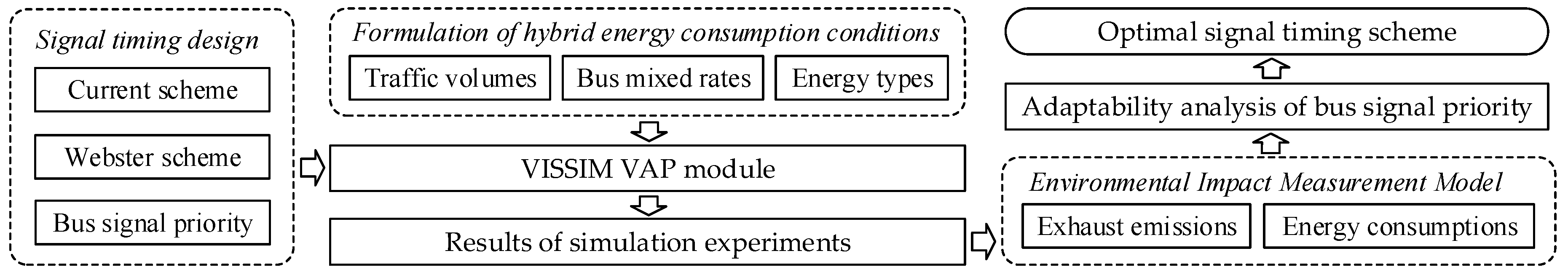
To analyze the adaptability of bus signal priority, a simulated-based evaluation method is proposed in this section, including the signal timing method for bus priority and measurement models for the operational cost of the intersection. A detailed illustration of the proposed method is given in
Figure 1.
3.1. Signal Timing Parameters for Bus Priority
Defining the shortest signal cycle
that stands for the shortest period of time for releasing all the vehicles arrived at the intersection during this period, it can be calculated as
where
is the total loss time within a cycle, s,
is sum of traffic flow ratios of each approach lane,
is the symbol for signal phase,
is the traffic flow ratio of phase
k,
is the current traffic volume of phase
k, pcu/h.
is the saturated traffic volume of phase
k, pcu/h.
is the start-up loss time, s.
is the interval of green time, s.
is the yellow time, s.
To coordinate the traffic flow arriving from different approach lanes, the experiential equation of the optimal signal cycle is introduced as follows:
where
is the optimal signal cycle, s.
As the optimization signal cycle
has been determined, the effective green time of the whole intersection and each phase can be derived by
where
is the total effective green time, s,
is the effective green time of phase
k, s.
As an essential step to ensuring bus signal priority will not affect normal operating of other approach lanes. The minimum green time
is often employed as a threshold to preliminarily judge whether current conditions are suitable for extending the green time or shorten the red time when a bus has been detected by the coil detector. Regarding pedestrian safety when crossing the intersection, an empirical minimum green time should be no shorter than usual walking time, which comes to the first constraint of phase
k as below.
where
is a minimum threshold of green time from a perspective of keeping pedestrians safe, s.
is the length of pavement which relates to phase
k, m and
is the walking speed of pedestrian, m/s.
Then, from the perspective of vehicle drivers, to avoid their second queuing in the approach lane when waiting for green time, it is also necessary to ensure all vehicles that arrived within the last signal cycle could pass through the intersection in the next green time. Thus, the second constraint could be formulated as
where
is another minimum threshold of green time to protect drivers’ rights, s.
is the distance between coil detector and stop line which relates to phase
k, m and
is the average headway of vehicles waiting in the intersection, m.
By combining the constraint and with the threshold of effective green time assigned for phase k simultaneously, the subject for minimum green time can be summarized as follows.
In addition, the green time cannot be extended without limit, which brings out the maximum green time
in bus signal priority. It can be formulated as follows:
3.2. Operational Cost Estimation
Different from the traditional bus priority timing optimization, which merely takes the minimum average capita delay as the objective, this paper further considers the impact of bus signal priority strategy on the operating conditions and emissions of buses and other vehicles at the intersection. A bus priority signal timing strategy is proposed with the aim of minimizing the overall delay and economic losses caused by vehicle emissions, in which the overall delay is reflected as the time cost while the emission loss is reflected as the environmental cost.
Take minimizing the total cost of intersection as the objective, as Equation (12).
where
is the total cost of the intersection, CNY,
is the time cost of the intersection, CNY,
is the environmental cost of the intersection, CNY.
Given the set of entrances of an intersection is
, the set of lanes on the
i-th entrance is
, the set of vehicle types
. The traffic volume of each lane could be collected through the coil sensor. Thus, the time cost of the intersection can be calculated as
where
,
are the average vehicle delays of buses and other vehicles in the lane
of entrance
respectively, s.
,
are the proportion of buses and other vehicles in the lane
of entrance
respectively, %.
,
are the capacity of buses and other vehicles respectively.
is the unit time value of passenger, CNY/s.
In addition, the equation of calculating the environmental cost of the intersection is also given as follows:
where
is the emission rate of pollutant
generated by vehicle type
in running condition
, g/s.
is the number of vehicles of type
in running condition
, pcu.
is the total travel time of vehicles of type
in running condition
, s.
is the unit environmental value of pollutant
, CNY/g.
3.3. Environmental Impact Measurement
3.3.1. VSP-based exhaust emissions measurement
VSP (vehicle-specific power) stands for the instantaneous power produced by a vehicle for each unit mass. Namely, for a given type of vehicle, VSP defines its required output power for moving each ton of mass [
37]. It should be noticed that VSP is not a constant value as it is closely related to the speed and acceleration of the vehicle. Thus, the exhaust emissions could be measured by VSP in light of conversion relations between output power and emissions. To estimate the impact of signal timing schemes on vehicle running conditions and emissions, the VSP-based exhaust emission measurement models with the consideration of energy consumption features of buses and other vehicles are employed.
According to the exhaust emission model for heavy trucks [
38], the technical parameters of buses collected in Beijing were further employed to characterize the running features of buses in actual traffic environments [
39]. The VSP formulation of buses is given as follows:
where
is the instantaneous speed of the vehicle, m/s.
is the instantaneous acceleration of the vehicle, m/s
2.
Palacios [
37] referenced the empirical coefficients to derive the VSP formulation of other vehicles, as Equation (16).
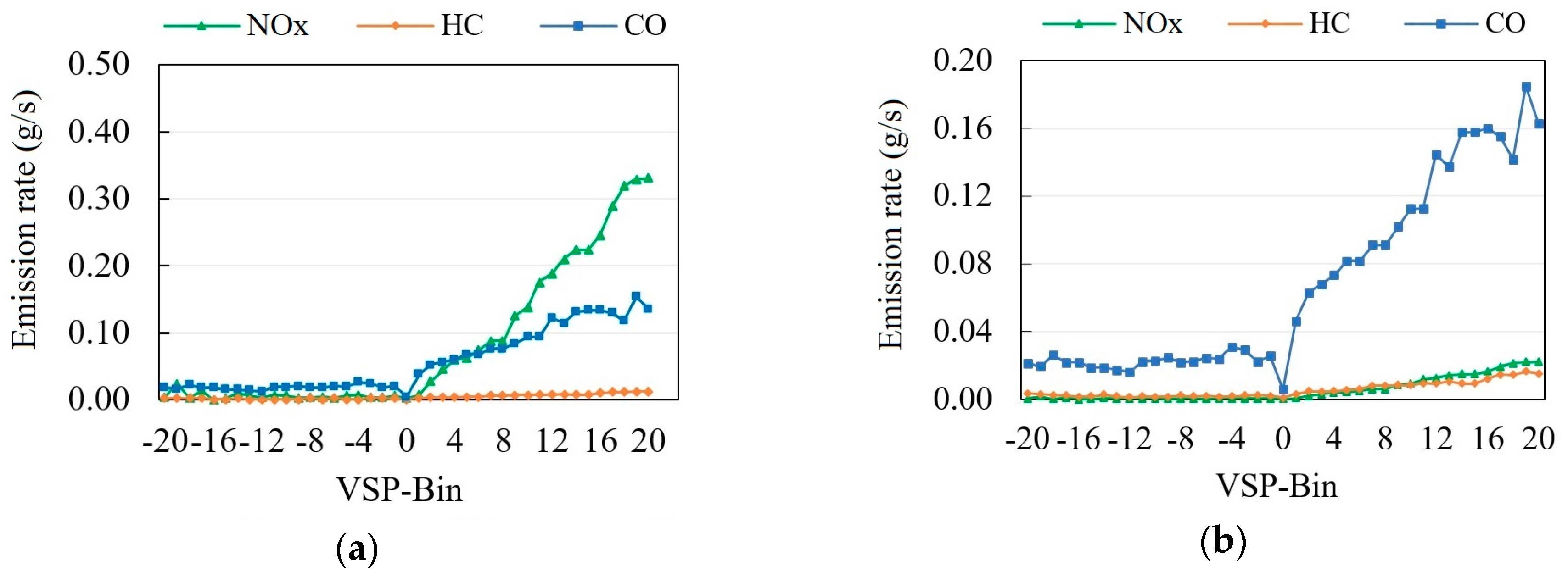
In engineering practice, calculating the VSP with instantaneous speed and acceleration poses great challenges in computing efficiency. To reduce the computation complexity with acceptable losses of accuracy, there is a consensus in discretizing the continuous function of VSP into specific ranges with the reference to the running conditions of vehicles, such as acceleration, deceleration, and idling. These obtained ranges are defined as VSP Bins, thereby reducing the dimension of the vehicle running record dataset effectively. Through the analysis of the emission features of different types of vehicles, the average emission rates of buses and other vehicles in each VSP Bin are given in
Figure 1, serving as the basis to measure vehicle emissions at the intersection.
It should be noticed that, the emissions mentioned in the study only concern the pollution gases which have been proven to be harmful to human health, such as NOx, HC, and CO. Although there are many potential factors (e.g., age of vehicle, type of engine) that may result in a difference in energy consumption performance, the reference values of emission rates used here aim to reflect a general situation for most vehicles according to an existing empirical study in Beijing, China [
39], which is supposed to best accord with the traffic conditions at intersections for subsequent simulation experiments.
As shown in
Figure 2, the emission rates of different pollutants is different but shows similar a variation trend. The minimum value of the emission rate that occurs near VSP equals 0, which means the emission rate of the pollutants is the lowest when the instantaneous speed of the vehicle is 0. If VSP is lower than 0, indicating that the vehicle is in a state of deceleration, the emission rates of three pollutants vary with VSP non-significantly when comparing with a uniform or acceleration state. If VSP is greater than 0, which means the vehicle is in a state of uniform or acceleration, the emission rates increase almost linearly with VSP and gradually emerge negative effects on the environment.
3.3.2. Energy consumption measurement
With the rapid development of the electric vehicle (EV) industry, EV has been widely regarded as an eco-friendly traffic mode for alleviating traffic emissions. Therefore, the penetration rate and energy consumption efficiency of EV should also be taken into consideration when evaluating the performance of signal timing strategies.
When under the running conditions of acceleration and deceleration, the instantaneous speed and acceleration are selected as two indicators to formulate a polynomial statistical regression model. When under the running conditions of uniform, the instantaneous speed is selected as the only indicator for model specification. When under the running condition of idling, the energy consumption is directly measured by the average emission coefficient. As such, the micro electricity and gasoline consumption rate measurement model could be given by [
40].
where
,
are the electricity and gasoline consumption rates, J/s and g/s.
,
,
are the multinomial regression coefficient function of acceleration, deceleration, uniform and idling running conditions respectively.
is the instantaneous speed of vehicle, km/h.
is the instantaneous acceleration of vehicle, m/s
2.
is the average emission coefficient in idling running condition, g/s.
Based on the data collected by the chassis dynamometer [
40], using the vehicle instantaneous speed and acceleration as input variables to calibrate the micro energy consumption model of an electric vehicle and the fuel consumption model of a gasoline vehicle. Corresponding regression coefficients in different running conditions of electric and gasoline vehicles are obtained in
Table 1.
By converting electricity consumption into standard coal, electricity consumption and gasoline consumption could be compared quantitatively. According to the monthly analysis report of China’s power industry in January 2013, the statistical result of average coal consumption from coal-fired power plants was 0.326 kg/(kWh), as the line loss in 2012 was about 6.62%. Thich means 1 kg standard coal can release 29,271 kJ of heat, and the equivalent electric power is 3600 kJ/(kWh). Thus, the average power generation efficiency of a coal-fired power plant in China can be estimated by Equation (18).
where
is the average power generation efficiency of coal, %.
Benefiting from the excellent performance of lithium battery technology, the charging and discharging efficiency reaches almost 97% for most vehicles in service [
40]. Therefore, the consumption rate of electricity can be converted into a standard coal consumption rate as follows.
where
is the energy efficiency of an electric vehicle, %.
is the coal consumption rate of an electric vehicle, g/s.
Similarly, since the value of gasoline conversion coefficient of standard coal is 1.4714, the consumption rate of gasoline can also be converted into the standard coal consumption rate as Equation (21).
where
is the coal consumption rate of a gasoline vehicle, g/s.
4. Results
Taking Equation (1) as the objective function, the VISSIM VAP module is taken to simulate the operating status of intersection under bus signal priority. The signal timing optimization is conducted for the different traffic scenarios under various combinations of traffic volumes and bus mixed rates. Through second-by-second simulation, the per-second vehicle speed and acceleration information are collected, so as to calculate the average capita delay and exhaust pollutant emissions in corresponding scenarios for further analysis of the adaptability of bus signal priority.
4.1. Basic Information of Chosen Intersection
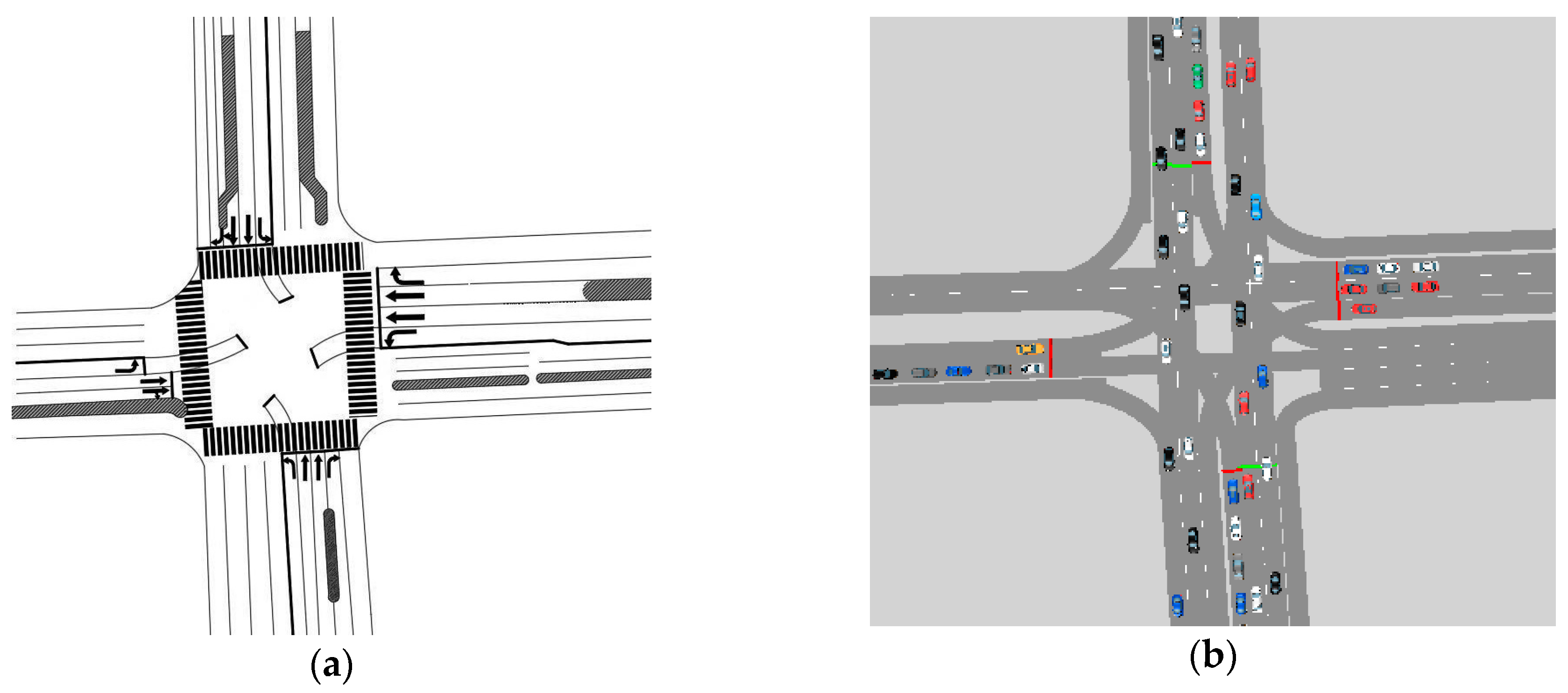
This paper selects the intersection of Suzhou Street as the analysis object. This intersection is located in the Haidian District of Beijing. It is a crossroad formed by the intersection of Suzhou Street and Haidian South Road, surrounded by residential areas such as Daozuomiao community, Wanggongfen community, and Suzhou Street apartment. At this intersection, the traffic volume is extremely high and nearly saturated, the flow directions are quite diverse, and the signal timing is complicated. The schematic diagram of the investigated intersection is shown in
Figure 3.
Through a field investigation, the current traffic volume at Suzhou Street intersection is 3625 pcu/h. In the North-South (NS) direction, a bus lane is located in a near-side lane, with 15% of bus mixed rate from south to north and 9% of bus mixed rate from north to south. The specific volumes for each approach lane are shown in
Table 2.
The current signal timing scheme investigated on-site and the calculated results of the Webster signal timing scheme are given in
Table 3.
According to Equations (9) and (10), the minimum and maximum green time of each phase can be obtained. Since the signal phase of N-S straight ahead is set for bus priority, there is no compressible green time for this phase. The compressible green time of the other three phases can be calculated by the difference between maximum green time and minimum green time. The sum of the compressible green time in one cycle is the final priority time of the bus, which is summarized in
Table 4.
4.2. Traffic Control Strategies Evaluation
From the public data of the Beijing Municipal Bureau of Statistics and the Social Security Bureau, the average wage of employees in Beijing in 2016 was 92,477 CNY and the average working time was 250 days within one year. Therefore, the time value used in the paper is regarded as 0.0128 CNY per second and the unit environmental cost of exhaust pollutants is 0.6 CNY/g [
41]. To evaluate the traffic performance of intersections under different signal timing schemes, three simulation experiments in the same traffic conditions were conducted for analysis. The calculation results of performance indicators such as average vehicle delay, average speed, total stopping times, etc., are presented in
Table 5.
In
Table 5, the Webster signal timing scheme can effectively reduce the average vehicle delay, increase the speed of the vehicle when passing through the intersection, and reduce the stopping times. However, bus signal priority will lead to a significant increase in average vehicle delay of the entire road network. The possible reason might be that the proportion of buses in the current traffic volume is relatively low. Once bus signal priority is applied, the delay of other vehicles in the remaining phases will increase, resulting in a small reduction in the average capita delay of the entire intersection. Besides, to evaluate the pollutant emissions performance of the intersection, the emission volumes of various pollutants and the emission resources from buses and other vehicles are shown in
Table 6.
In
Table 6, the Webster signal timing scheme and the bus priority signal timing scheme both lead to an increase in the total amount of exhaust pollutants at the intersection. While the total emissions of bus exhaust pollutants are reduced, we can see a significant increase in the total emissions of other vehicles. Therefore, how to balance the relationship between traffic efficiency and pollutant emissions still needs to be discussed in more situations. Next, we analyze the operating status of intersection under different bus mixed rates with current traffic volume. The comparison of traffic performance is given in
Table 7.
As shown in
Table 7, when the bus mixed rate is 20%, the optimization effect of bus signal priority for the whole road network is more appreciable, which makes stopping times significantly reduced. When the bus mixed rate is lower than 15%, the performance of the bus signal priority is not obvious. When the bus mixed rate exceeds 40%, the increase in average vehicle delay keeps growing, also resulting in a decrease in travel speed. Therefore, if only time cost is taken into consideration with current traffic volume, when the bus mixed rate is less than 20%, the current signal timing scheme should be the best choice. However, when the bus mixed rate exceeds 20%, the bus priority signal timing scheme can effectively reduce average vehicle and capita delay. Hence, bus signal priority should be chosen. Moreover, the comparison of pollutant emission performance is presented as follows.
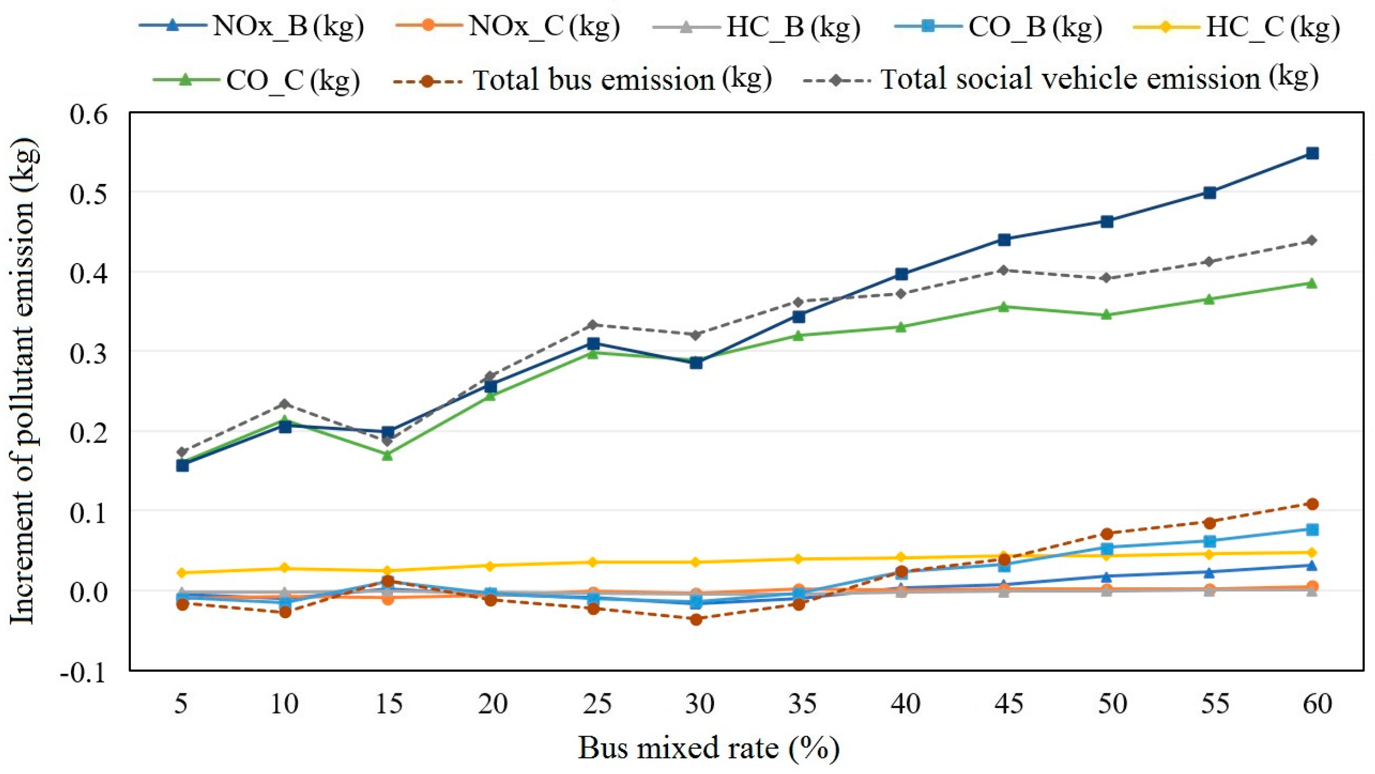
To compare the emissions of current and bus priority signal timing schemes more intuitively, a line chart for describing the increment of pollutant emissions is presented in
Figure 4.
As known from
Table 8 and
Figure 4, with the increase of bus mixed rate, the emission of each pollutant keeps rising, and the increment grows with bus mixed rate. When the bus mixed rate is greater than 30%, the increment of the total amount of exhaust pollutants at the intersection rises linearly. When the bus mixed rate is 5% and 15%, the total emissions of exhaust pollutants increase least, compared with the current signal timing scheme.
4.3. Adaptability Analysis of Bus Signal Priority
By crossing typical traffic volumes, bus mixed rates and energy consumption types, 96 combined traffic scenarios were formed. Among them, the traffic volumes are 2000, 3000, 4000, 5000 pcu/h, respectively, a total of four cases. The bus mixed rates are 5%, 10%, 15%, 20%, 25%, 30%, 35%, 40%, 45%, 50%, 55%, and 60%, respectively, a total of 12 cases. The energy consumption types include two categories of gasoline and electricity. Each scenario was then simulated in VISSIM to analyze the performance of indicators such as vehicle delays, exhaust emissions and the overall costs of the intersection.
Assuming that the average passenger capacity of buses and other vehicles is 30 and 1.5, respectively. Based on the vehicle running detailed records output from VISSIM, the variations of time and environmental cost could be calculated for analysis.
4.3.1. Time Cost Analysis
At first, the adaptability of bus signal priority is evaluated from the perspective of time cost.
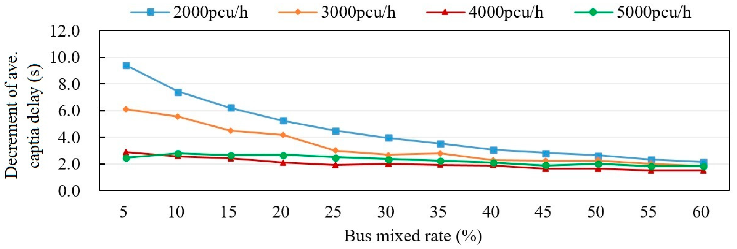
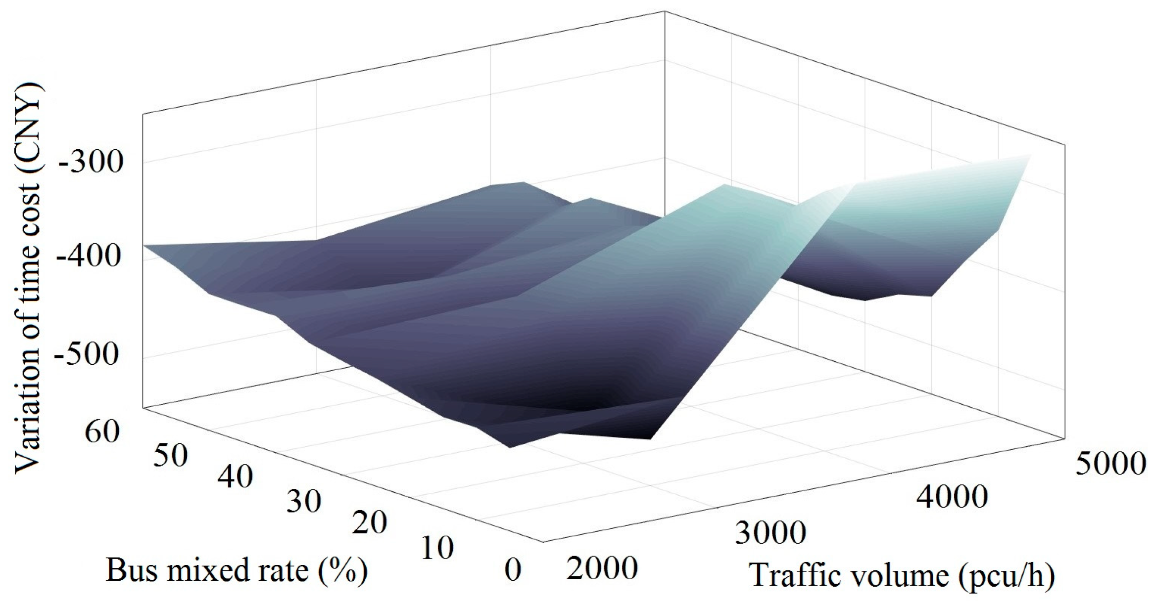
Figure 5 gives the decrements of average capita delay between current and bus priority signal timing schemes in different traffic scenarios. Moreover,
Figure 6 shows the converted time cost of the intersection.
As shown in
Figure 5 and
Figure 6, when the traffic volume at the intersection is 2000 pcu/h, the bus signal priority has a significant effect on improving the traffic conditions, which greatly reduces the average capita delay. In addition, when the bus mixed rate is 5%, the decrement of delay turns to be the highest. When the traffic volume is 3000 pcu/h, bus signal priority could reduce the average capita delay and save total time cost regardless of bus mixed rates. When the traffic volume is 4000 pcu/h, although bus signal priority can reduce average capita delay, the decrement is still lower than those under previous traffic volumes. When the traffic volume comes to 5000 pcu/h, the effects of bus signal priority on reducing average capita delay become not obvious and gradually weaken with the increase of the bus mixed rates.
4.3.2. Environmental Cost Analysis
Next, in the aspect of environmental effect, the adaptability of bus signal priority could be further evaluated.
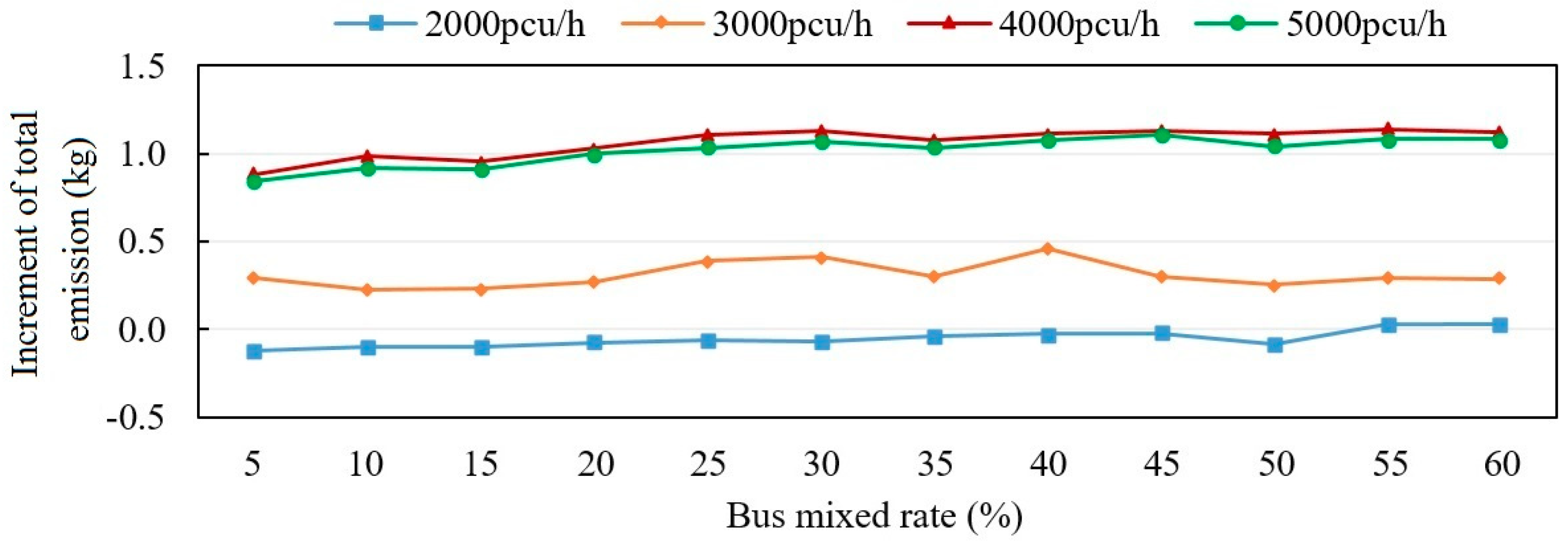
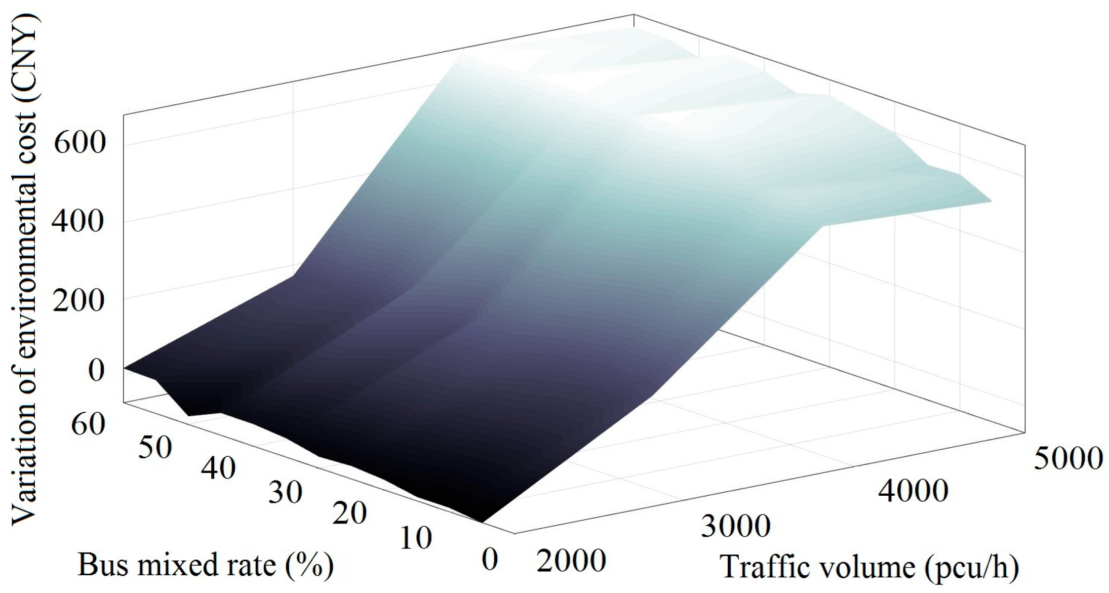
Figure 7 is the increment of total vehicle emissions between current and bus priority signal timing schemes in different traffic scenarios. Moreover, the variation of environmental cost is presented in
Figure 8.
Figure 7 and
Figure 8 show that, when the traffic volume is 2000 pcu/h, the difference of exhaust pollutant emission volumes between current and bus priority signal timing schemes decreases first and then increases with the rise of bus mixed rates. Therefore, when the bus mixed rate is comparatively low, both exhaust pollutants emissions and environmental cost could be reduced by introducing bus signal priority. When the traffic volume is 3000 pcu/h, the total amount of vehicle exhaust emissions varies in volatility and if bus mixed rate is between 10% and 20%, the emissions increase the least. When the traffic volume at the intersection reaches 4000 pcu/h, bus signal priority will lead to a large increase in vehicle exhaust emissions. When the traffic volume rises up to 5000 pcu/h, bus signal priority results in an increase in both total amount of exhaust emissions and the whole environmental cost. Besides, the increment of environmental cost grows fast with the rise of bus mixed rate.
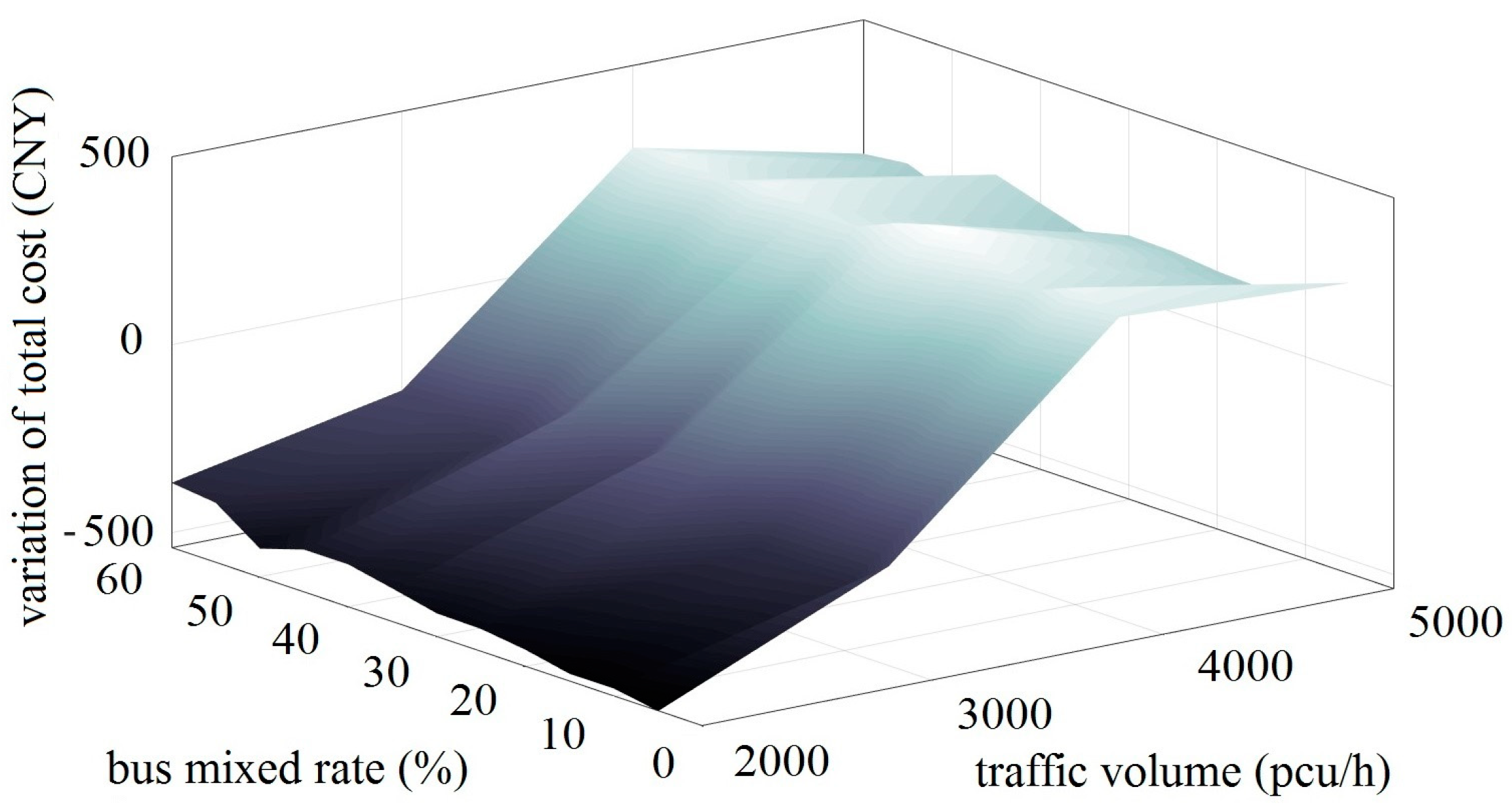
4.3.3. Total Operational Cost Analysis
In
Figure 9, the statistics of total cost considering both traffic and environmental effects at the intersection are performed. When the traffic volume is within 2000 to 3000 pcu/h, the time and environmental costs tend to increase slightly with the rise of bus mixed rate. While under that traffic volume, no matter what bus mixed rate would be, the total cost of the intersection could be significantly reduced, indicating that bus signal priority presents an obvious optimization effect in these traffic conditions. When the traffic volume increases to 4000–5000 pcu/h, the total cost is larger than that of the current signal timing scheme, which means bus priority strategy cannot effectively improve the average capita delay and emissions anymore. As a result, when the traffic volume is comparatively large, the bus priority signal timing scheme becomes inapplicable.
4.3.4. Energy Consumption Efficiency Analysis
To compare the energy consumption efficiency of electric and gasoline vehicles objectively, the standard coal consumption rate of two energy consumption types was deemed as a uniform standard in this part. With reference to previous work [
40], the energy consumption coefficients of normal vehicles are employed to evaluate electricity consumption efficiency. Since the development of an electric bus is still under a promotion stage in most cities with an immature standard and many unstable technical parameters, especially in the energy consumption aspect, the buses were excluded when calculating the overall coal consumption efficiency, which means only other social vehicles were supposed to be powered by electricity in simulation experiments. The statistical results of 10 samples randomly selected from the above 96 scenarios are presented in
Table 9.
It can be seen from
Table 9 that when under the same conditions, the average electricity and gasoline consumption rates are 2.832 × 10
5 J/s and 52.129 g/s, respectively. To be more intuitive, the converted standard coal consumption rates are further calculated, which turn to be 28.312 and 76.702 g/s. In this regard, the coal consumption rates of electric power are only 36.9% of those of gasoline power. By adjusting the proportion of electric vehicles in all vehicles, it is possible to reduce the emissions of vehicle exhaust pollutants at intersections without affecting normal traffic efficiency. The higher the proportion of electric vehicles is, the better the optimization results for the entire intersection will be, which also demonstrates the practicability of the electric vehicle’s future development.
5. Conclusions
This study integrates the environmental concern into signal timing strategy design aiming at providing implications for traffic control practice. A comprehensive adaptability analysis of bus priority strategy under hybrid energy consumption conditions that consist of various levels of traffic volumes, bus mixed rates, and vehicle energy types was presented to explore an efficient and eco-friendly solution for traffic policymakers. It is discovered that bus priority strategy at the intersection often performs well in improving the operating efficiency of buses and considerably reducing average capita delays. In the meanwhile, it may also lead to an increase in delays of other vehicles and the deterioration of vehicle running conditions, thereby increasing the emissions of exhaust pollutants at the entire intersection and resulting in adverse environmental impacts.
To find a balance between efficient and environmental care, a framework of evaluating the environment effects of bus signal priority was proposed, which not only facilitates deciding whether a bus signal priority is suitable to be implemented at target intersection in current traffic conditions, but also fills the research gap regarding incorporating environmental concern in traditional signal timing optimization problem. From the results of the case study, it turns out that, when the traffic volume is relatively small, approximately 2000–3000 pcu/h, bus signal priority improves the traffic efficiency of intersection significantly. While along with the increase in the bus mixed rate, the optimization effect gradually weakens. When the traffic volume is relatively large, about 4000–5000 pcu/h, the decrease of time cost resulting from bus signal priority cannot offset the increase of the environmental cost, which leads to an increase in the total cost of the entire intersection. Moreover, the introduction of electric vehicles improves the current carbon emission status of intersections significantly. The average electricity and gasoline consumption rates are 2.832 × 10⁵ J/s and 52.129 g/s respectively, and the equivalent coal consumption could be cut by 63.09%. It also proves that the promotion of replacing traditional gasoline vehicles with electric vehicles is a feasible way of alleviating traffic pollution at intersections, which deserves more attention in future traffic control practice.
Author Contributions
Conceptualization, N.H.; investigation, Z.W.; data curation, Y.F.; methodology, N.H. and E.Y.; software, Y.F.; validation, E.Y.; supervision, E.Y.; writing—original draft, N.H., Y.F. and Z.W.; writing—review & editing, N.H.; funding acquisition, E.Y.
Funding
This research was funded by the National Key R&D Program of China (No. 2018YFB1201601) and the Fundamental Research Funds for the Central Universities (No. 2019YJS102 and No. 2019JBZ107).
Conflicts of Interest
The authors declare no conflict of interest.
References
- Tischer, V.; Fountas, G.; Polette, M.; Rye, T. Environmental and economic assessment of traffic-related air pollution using aggregate spatial information: A case study of Balneário Camboriú, Brazil. J. Transp. Health 2019, 14, 100592. [Google Scholar] [CrossRef]
- Lin, C.; Zhou, X.; Wu, D.; Gong, B. Estimation of Emissions at Signalized Intersections Using an Improved MOVES Model with GPS Data. Int. J. Environ. Res. Public Health 2019, 16, 3647. [Google Scholar] [CrossRef]
- Tezel, N.M.; Sari, D.; Ozkurt, N.; Keskin, S.S. Combined NOx and noise pollution from road traffic in Trabzon, Turkey. Sci. Total Environ. 2019, 696, 134044. [Google Scholar] [CrossRef]
- Piscitelli, P.; Valenzano, B.; Rizzo, E.; Maggiotto, G.; Rivezzi, M.; Esposito Corcione, F.; Miani, A. Air Pollution and Estimated Health Costs Related to Road Transportations of Goods in Italy: A First Healthcare Burden Assessment. Int. J. Environ. Res. Public Health 2019, 16, 2876. [Google Scholar] [CrossRef]
- Barnes, J.H.; Chatterton, T.J.; Longhurst, J.W.S. Emissions vs exposure: Increasing injustice from road traffic-related air pollution in the United Kingdom. Transport. Res. D Transp. Environ. 2019, 73, 6–66. [Google Scholar] [CrossRef]
- Liu, Y.; Lan, B.; Shirai, J.; Austin, E.; Yang, C.; Seto, E. Exposures to Air Pollution and Noise from Multi-Modal Commuting in a Chinese City. Int. J. Environ. Res. Public Health 2019, 16, 2539. [Google Scholar] [CrossRef] [PubMed]
- Pathivada, B.K.; Perumal, V. Analyzing dilemma driver behavior at signalized intersection under mixed traffic conditions. Transp. Res. F Traffic Psychol. Behav. 2019, 60, 111–120. [Google Scholar] [CrossRef]
- Xu, C.; Dong, D.; Ou, D.; Ma, C. Time-of-Day Control Double-Order Optimization of Traffic Safety and Data-Driven Intersections. Int. J. Environ. Res. Public Health 2019, 16, 870. [Google Scholar] [CrossRef]
- Anderson, P.; Daganzo, C.F. Effect of transit signal priority on bus service reliability. Transp. Res. B Meth. 2019. (In press) [Google Scholar] [CrossRef]
- Goh, K.C.K.; Currie, G.; Sarvi, M.; Logan, D. Bus accident analysis of routes with/without bus priority. Accident Anal. Prev. 2014, 65, 18–27. [Google Scholar] [CrossRef]
- Viegas, J.; Lu, B. The Intermittent Bus Lane signals setting within an area. Transp. Res. C 2004, 12, 453–469. [Google Scholar] [CrossRef]
- Zhang, W.-H.; Lu, H.-P. Analysis of Vehicle Delays in Public Traffic Priority Pre-Signal Control Intersections. China J. Highw. Transp. 2005, 4, 78–82. [Google Scholar]
- Skabardonis, A. Control Strategies for Transit Priority. Transp. Res. Rec. J. Transp. Res. Board 2007, 1727, 20–26. [Google Scholar] [CrossRef]
- Zyryanov, V.; Mironchuk, A. Simulation Study of Intermittent Bus Lane and Bus Signal Priority Strategy. In Proceedings of the Social and Behavioral Sciences, Conference on Transport Research Arena, Athens, Greece, 23–26 April 2012. [Google Scholar]
- Xiong, C.-F.; Lv, Z.-L.; Ye, Y. Research on Bus Priority Signal Control Optimization Method Considering Emission Factors. J. Transp. Info. Saf. 2012, 30, 75–79. [Google Scholar]
- Ye, X.-C.; Ma, W.-J. Influence of Access Traffic on the Operational Efficiencies of Bus Lane and Main Road. In Proceedings of the Social and Behavioral Sciences, 13th COTA International Conference of Transportation Professionals (CICTP), Shenzhen, China, 13–16 August 2013. [Google Scholar]
- Guler, S.I.; Gayah, V.V.; Menendez, M. Bus priority at signalized intersections with single-lane approaches: A novel pre-signal strategy. Transp. Res. C 2016, 63, 51–70. [Google Scholar] [CrossRef]
- Elias, W.J. The Greenback Experiment-Signal Pre-emption for Express Buses: A Demonstration Project. In Report DMT-014; California Department of Transportation: Sacramento, CA, USA, 1976. [Google Scholar]
- Salter, R.J.; Shahi, J. Prediction of effects of bus-priority schemes by using computer simulation techniques. Transp. Res. Rec. 1979, 718, 1–5. [Google Scholar]
- Dion, F.; Hellinga, B. A rule-based real-time traffic responsive signal control system with transit priority: Application to an isolated intersection. Transp. Res. B 2002, 36, 325–343. [Google Scholar] [CrossRef]
- He, Q.; Head, K.L.; Ding, J. Multi-modal traffic signal control with priority, signal actuation and coordination. Transp. Res. C Emerg. Technol. 2014, 46, 65–82. [Google Scholar] [CrossRef]
- Ma, X.-H.; Liu, X.-M.; Zhang, J.-J. Traffic Signal Control of Over-Saturation Intersection Considering Bus Priority. J. Jilin Univ. Eng. Sci. 2015, 45, 748–754. [Google Scholar]
- Zhou, L.; Wang, Y.-Z.; Liu, Y.-D. Active signal priority control method for bus rapid transit based on Vehicle Infrastructure Integration. Int. J. Transp. Sci. Technol. 2017, 6, 99–109. [Google Scholar] [CrossRef]
- Wu, K.; Guler, S.I. Estimating the impacts of transit signal priority on intersection operations: A moving bottleneck approach. Transp. Res. C 2019, 105, 346–358. [Google Scholar] [CrossRef]
- Viegas, J.; Baichuan, L. Widening the scope for bus priority with intermittent bus lanes. Transp. Plan. Technol. 2000, 24, 87–110. [Google Scholar] [CrossRef]
- Guan, W.; Shen, J.-S.; Ge, F. Study on Signal Control Strategy of Bus Priority. J. Syst. Eng. 2001, 3, 176–180. [Google Scholar]
- Zhang, W.-H.; Lu, H.-P.; Liu, Q. Discussion on Evaluation Index System of Public Transport Priority Passage Measures. Trafc. Stdn. 2004, 11, 85–89. [Google Scholar]
- Christofa, E.; Skabardonis, A. Traffic signal optimization with application of transit signal priority to an isolated intersection. Transp. Res. Rec. J. Transp. Res. Board 2011, 2259, 192–201. [Google Scholar] [CrossRef]
- Ahmed, F.; Hawas, Y.E. An integrated real-time traffic signal system for transit signal priority, incident detection and congestion management. Transp. Res. C Emerg. Technol. 2015, 60, 52–76. [Google Scholar] [CrossRef]
- Zeng, X.-S.; Zhang, Y.-L.; Balke, K.N.; Yin, K. A real-time transit signal priority control model considering stochastic bus arrival Time. IEEE Trans. Intell. Transp. Syst. 2014, 15, 1657–1666. [Google Scholar] [CrossRef]
- Li, M.; Yin, Y.-F.; Zhou, K.; Zhang, W.-B.; Liu, H.-C.; Tan, C.-W. Adaptive Transit Signal Priority on Actuated Signalized Corridors. In Proceedings of the 84th Transportation Research Board Annual Meeting, Washington, DC, USA, 9–13 January 2005. [Google Scholar]
- Zhou, S.-P. Research on Traffic Signal Control Strategy at Urban Intersection Considering Emission Factors. Ph.D. Thesis, Wuhan University of Technology, Wuhan, China, 1 May 2009. [Google Scholar]
- Zhang, L.-H.; Yin, Y.-F.; Chen, S.-G. Robust signal timing optimization with environmental concerns. Transp. Res. C 2013, 29, 55–71. [Google Scholar] [CrossRef]
- Zheng, L.; Xu, C.-C.; Jin, P.J.; Ran, B. Network-wide signal timing stochastic simulation optimization with environmental concerns. Appl. Soft Comput. 2019, 77, 678–687. [Google Scholar] [CrossRef]
- Xiong, C.-F. Research on Bus Priority Control Strategy Considering Emission Factors. Master’s Thesis, Guangxi University, Guangxi, China, June 2012. [Google Scholar]
- Rao, Q.; Zhang, L.; Yang, W.-C.; Zhang, M. A traffic emission-saving signal timing model for urban isolated intersections. In Proceedings of the Social and Behavioral Sciences, 13th COTA International Conference of Transportation Professionals (CICTP), Shenzhen, China, 13–16 August 2013. [Google Scholar]
- Palacios, J. Understanding and Quantifying Motor Vehicle Emissions with Vehicle Specific Power and TILDAS Remote Sensing. Ph.D. Thesis, Massachusetts Institute of Technology, Cambridge, MA, USA, 1999. [Google Scholar]
- Andrei, P. Real World Heavy-Duty Vehicle Emission Modeling. Master’s Thesis, West Virginia University, Morgantown, West Virginia, WA, USA, 2001. [Google Scholar]
- Liu, Q.-X. Research on the Influence of Bus Signal Priority Strategy on Exhaust Emission Based on Micro Simulation. Master’s Thesis, Beijing Jiaotong University, Beijing, China, June 2012. [Google Scholar]
- Yao, E.-J.; Lang, Z.-F.; Song, Y.-Y.; Yang, Y.; Zuo, T.; Wang, W.-H. Microscopic Driving Parameters-Based Energy-Saving Effect Analysis under Different Electric Vehicle Penetration. Adv. Mech. Eng. 2013, 5, 435721. [Google Scholar] [CrossRef]
- Wu, D.-D.; Shao, Y.; Jing, Q.-P.; Huo, Z.-B. Evaluation of ecological economic value loss caused by traffic congestion in Beijing. Ecol. Econ. 2013, 4, 75–79. [Google Scholar]
Figure 1.
Flow chart of the simulation-based evaluation method.
Figure 1.
Flow chart of the simulation-based evaluation method.
Figure 2.
VSP-based pollutant emission rates: (a) For buses, (b) for other vehicles.
Figure 2.
VSP-based pollutant emission rates: (a) For buses, (b) for other vehicles.
Figure 3.
Schematic diagram of the investigated intersection: (a) Description of intersection canalization drawn by AutoCAD with the measurement data obtained from the on-site investigation, (b) description of simulation interface at the chosen intersection generated by VISSIM.
Figure 3.
Schematic diagram of the investigated intersection: (a) Description of intersection canalization drawn by AutoCAD with the measurement data obtained from the on-site investigation, (b) description of simulation interface at the chosen intersection generated by VISSIM.
Figure 4.
Increment of pollutant emissions under different bus mixed rates.
Figure 4.
Increment of pollutant emissions under different bus mixed rates.
Figure 5.
Decrement of average capita delay under different traffic conditions.
Figure 5.
Decrement of average capita delay under different traffic conditions.
Figure 6.
Variation of time cost in different traffic scenarios
Figure 6.
Variation of time cost in different traffic scenarios
Figure 7.
Increment of total emissions under different traffic scenarios.
Figure 7.
Increment of total emissions under different traffic scenarios.
Figure 8.
Variation of environmental cost in different traffic scenarios.
Figure 8.
Variation of environmental cost in different traffic scenarios.
Figure 9.
Variation of total cost in different traffic scenarios.
Figure 9.
Variation of total cost in different traffic scenarios.
Table 1.
Energy consumption regression coefficients of electric and gasoline vehicles under different running conditions.
Table 1.
Energy consumption regression coefficients of electric and gasoline vehicles under different running conditions.
| Variable 1 | Electric Vehicle 2 | Gasoline Vehicle 2 |
|---|
| Acce. | Dece. | Unif. | Idl. | Acce. | Dece. | Unif. | Idl. |
|---|
| intercept | 2.17 × 10³ | 1.45 × 10³ | 1.89 × 10³ | 1.89 × 10³ | 5.00 × 10⁻¹ | 2.69 × 10⁻¹ | 4.00 × 10⁻¹ | 2.65 × 10⁻¹ |
| −9.41 × 101 | 3.09 × 101 | - | - | - | 1.40 × 10⁻² | - | - |
| 4.99 × 100 | - | 1.81× 100 | 1.81 × 100 | - | - | 9.22 × 10⁻⁵ | - |
| −2.50 × 10⁻² | 2.10 × 10⁻² | - | - | 9.13 × 10⁻⁷ | 2.55 × 10⁻⁶ | - | - |
| −1.16 × 10² | - | - | - | - | 6.94 × 10⁻³ | - | - |
| 9.73 × 100 | - | - | - | - | 3.09 × 10⁻⁴ | - | - |
| - | - | - | - | 2.51 × 10⁻⁵ | - | - | - |
| 6.22 × 101 | - | - | - | 2.20 × 10⁻³ | - | - | - |
| −1.12 × 100 | 1.88 × 10⁻¹ | - | - | −6.26 × 10⁻⁵ | - | - | - |
| 9.52 × 10⁻³ | - | - | - | - | - | - | - |
| −4.29 × 10⁻¹ | 1.02 × 10⁻¹ | - | - | - | 1.65 × 10⁻⁵ | - | - |
| - | −6.33 × 10⁻³ | - | - | - | - | - | - |
| - | 2.14 × 10⁻⁴ | - | - | - | - | - | - |
| - | 5.00 × 10⁻³ | - | - | - | −6.24 × 10⁻⁸ | - | - |
| −7.72 × 10⁻⁵ | 3.86 × 10⁻⁴ | - | - | - | - | - | - |
| - | - | - | - | - | - | - | - |
Table 2.
Statistics of traffic volume of approach lanes at the investigated intersection.
Table 2.
Statistics of traffic volume of approach lanes at the investigated intersection.
| Approach Lane | Vehicle Type | Left Turn (pcu/h) | Straight Ahead (pcu/h) | Right Turn (pcu/h) |
|---|
| South side | Bus | - | 45 | - |
| Other vehicles | 92 | 253 | 96 |
| East side | Bus | - | - | - |
| Other vehicles | 227 | 421 | 67 |
| North side | Bus | - | - | - |
| Other vehicles | 207 | 665 | 624 |
| West side | Bus | - | - | - |
| Other vehicles | 292 | 235 | 113 |
Table 3.
Current and Webster signal timing schemes.
Table 3.
Current and Webster signal timing schemes.
| Order | Signal Phase | Direction | Green Time (s) | Cycle Length (s) |
|---|
| Current | Webster | Current | Webster |
|---|
| 1 | Straight ahead | N-S | 31 | 61 | 167 | 187 |
| 2 | Left turn | N-S | 22 | 33 |
| 3 | Straight ahead | E-W | 51 | 33 |
| 4 | Left turn | E-W | 41 | 45 |
Table 4.
Bus priority timing parameters
Table 4.
Bus priority timing parameters
| Signal Phase | Direction | Maximum Green Time (s) | Minimum Green Time (s) | Compressible Green Time (s) | Bus Priority Time (s) |
|---|
| Straight ahead | N-S | 63 | 31 | - | 50 |
| Left turn | N-S | 35 | 22 | 13 |
| Straight ahead | E-W | 35 | 22 | 13 |
| Left turn | E-W | 47 | 23 | 24 |
Table 5.
Traffic performance under different signal timing schemes
Table 5.
Traffic performance under different signal timing schemes
| Indicator | Signal Timing Scheme |
|---|
| Current | Webster | Bus Priority |
|---|
| Ave. vehicle delay (s) | 40.57 | 39.50 | 40.03 |
| Ave. speed (km/h) | 10.16 | 10.33 | 10.25 |
| Ave. stopping times | 0.55 | 0.52 | 0.53 |
| Ave. stopping time (s) | 36.56 | 35.52 | 36.04 |
| Tot. vehicle delay (s) | 1.37 × 10⁵ | 1.43 × 10⁵ | 1.40 × 10⁵ |
| Tot. travel distance (km) | 573 | 608 | 590 |
| Tot. travel time (s) | 2.03 × 10⁵ | 2.12 × 10⁵ | 2.07 × 10⁵ |
| Tot. stopping times | 1856 | 1872 | 1864 |
| Tot. stopping time (s) | 1.26 × 10⁵ | 1.28 × 10⁵ | 1.24 × 10⁵ |
Table 6.
Pollutant emission performance under different signal timing schemes
Table 6.
Pollutant emission performance under different signal timing schemes
| Indicator | Signal Timing Scheme |
|---|
| Current | Webster | Bus Priority |
|---|
| NOx_B (kg) | 0.087 | 0.084 | 0.077 |
| NOx_C (kg) | 0.261 | 0.275 | 0.253 |
| HC_B (kg) | 0.014 | 0.013 | 0.012 |
| HC_C (kg) | 0.402 | 0.425 | 0.432 |
| CO_B (kg) | 0.157 | 0.155 | 0.145 |
| CO_C (kg) | 4.760 | 5.021 | 4.990 |
| Tot. emission of buses (kg) | 0.258 | 0.251 | 0.233 |
| Tot. emission of other vehicles (kg) | 5.423 | 5.720 | 5.674 |
Table 7.
Comparison of traffic performance under different bus mixed rates.
Table 7.
Comparison of traffic performance under different bus mixed rates.
| Bus Mixed Rate | Current Signal Timing Scheme | Bus Priority Signal Timing Scheme |
|---|
| Ave. Vehicle Delay(s) | Ave. Capita Delay(s) | Ave. Stopping Times | Ave. Speed (km/h) | Ave. Vehicle Delay(s) | Ave. Capita Delay(s) | Ave. Stopping Times | Ave. Speed (km/h) |
|---|
| 5% | 31.73 | 16.27 | 0.54 | 10.22 | 31.87(0.14↑) 1 | 15.94(0.33↓) 2 | 0.54 | 9.21 |
| 10% | 31.54 | 13.20 | 0.54 | 10.26 | 31.66(0.12↑) | 12.67(0.53↓) | 0.54 | 9.22 |
| 15% | 31.38 | 11.08 | 0.53 | 10.28 | 31.45(0.07↑) | 10.49(0.59↓) | 0.53 | 9.23 |
| 20% | 31.11 | 9.67 | 0.56 | 10.27 | 31.24(0.13↑) | 8.93(0.74↓) | 0.56 | 9.24 |
| 25% | 30.94 | 8.54 | 0.54 | 10.37 | 30.53(0.41↓) | 7.66(0.88↓) | 0.54 | 9.37 |
| 30% | 30.99 | 7.73 | 0.53 | 10.36 | 30.67(0.32↓) | 6.82(0.91↓) | 0.53 | 9.34 |
| 35% | 31.12 | 7.08 | 0.53 | 10.29 | 30.65(0.47↓) | 6.14(0.94↓) | 0.53 | 9.32 |
| 40% | 30.96 | 6.54 | 0.53 | 10.28 | 30.55(0.41↓) | 5.56(0.98↓) | 0.53 | 9.34 |
| 45% | 31.03 | 6.09 | 0.53 | 10.30 | 30.85(0.18↓) | 5.16(0.93↓) | 0.53 | 9.22 |
| 50% | 30.98 | 5.67 | 0.53 | 10.30 | 30.72(0.26↓) | 4.74(0.94↓) | 0.53 | 9.23 |
| 55% | 30.68 | 5.28 | 0.52 | 10.38 | 30.52(0.16↓) | 4.36(0.92↓) | 0.52 | 9.28 |
| 60% | 30.86 | 5.04 | 0.52 | 10.33 | 30.46(0.40↓) | 4.06(0.98↓) | 0.52 | 9.29 |
Table 8.
Comparison of pollutant emission performance under different bus mixed rates.
Table 8.
Comparison of pollutant emission performance under different bus mixed rates.
| Bus Mixed Rate | Signal Timing Scheme | NOx_B (kg) | NOx_C (kg) | HC_B (kg) | HC_C (kg) | CO_B (kg) | CO_C (kg) | Total Emissions (kg) |
|---|
| Buses | Other Vehicles |
|---|
| 5% | Cur. | 0.042 | 0.270 | 0.007 | 0.417 | 0.075 | 4.944 | 0.124 | 5.631 |
| Bus Pri. | 0.037 | 0.260 | 0.005 | 0.440 | 0.066 | 5.106 | 0.108 | 5.806 |
| 10% | Cur. | 0.088 | 0.262 | 0.014 | 0.402 | 0.157 | 4.778 | 0.259 | 5.442 |
| Bus Pri. | 0.078 | 0.254 | 0.012 | 0.430 | 0.142 | 4.992 | 0.232 | 5.676 |
| 15% | Cur. | 0.109 | 0.258 | 0.017 | 0.397 | 0.194 | 4.716 | 0.320 | 5.371 |
| Bus Pri. | 0.111 | 0.249 | 0.017 | 0.422 | 0.205 | 4.886 | 0.333 | 5.557 |
| 20% | Cur. | 0.149 | 0.250 | 0.024 | 0.383 | 0.273 | 4.547 | 0.446 | 5.180 |
| Bus Pri. | 0.144 | 0.244 | 0.022 | 0.414 | 0.269 | 4.790 | 0.435 | 5.448 |
| 25% | Cur. | 0.182 | 0.242 | 0.030 | 0.369 | 0.337 | 4.389 | 0.549 | 5.000 |
| Bus Pri. | 0.173 | 0.241 | 0.027 | 0.405 | 0.327 | 4.687 | 0.527 | 5.333 |
| 30% | Cur. | 0.215 | 0.237 | 0.035 | 0.361 | 0.395 | 4.293 | 0.645 | 4.891 |
| Bus Pri. | 0.198 | 0.233 | 0.031 | 0.397 | 0.381 | 4.582 | 0.610 | 5.212 |
| 35% | Cur. | 0.244 | 0.230 | 0.040 | 0.352 | 0.450 | 4.194 | 0.734 | 4.776 |
| Bus Pri. | 0.234 | 0.232 | 0.036 | 0.392 | 0.447 | 4.514 | 0.717 | 5.138 |
| 40% | Cur. | 0.257 | 0.226 | 0.043 | 0.344 | 0.480 | 4.104 | 0.780 | 4.674 |
| Bus Pri. | 0.260 | 0.227 | 0.041 | 0.385 | 0.503 | 4.435 | 0.804 | 5.047 |
| 45% | Cur. | 0.284 | 0.222 | 0.047 | 0.337 | 0.527 | 4.022 | 0.858 | 4.581 |
| Bus Pri. | 0.291 | 0.224 | 0.046 | 0.381 | 0.560 | 4.377 | 0.897 | 4.982 |
| 50% | Cur. | 0.307 | 0.217 | 0.051 | 0.329 | 0.573 | 3.930 | 0.931 | 4.476 |
| Bus Pri. | 0.325 | 0.219 | 0.051 | 0.372 | 0.627 | 4.276 | 1.003 | 4.867 |
| 55% | Cur. | 0.324 | 0.213 | 0.054 | 0.321 | 0.609 | 3.852 | 0.987 | 4.386 |
| Bus Pri. | 0.347 | 0.215 | 0.055 | 0.367 | 0.671 | 4.217 | 1.073 | 4.799 |
| 60% | Cur. | 0.339 | 0.207 | 0.057 | 0.314 | 0.642 | 3.768 | 1.038 | 4.289 |
| Bus Pri. | 0.371 | 0.212 | 0.058 | 0.362 | 0.719 | 4.153 | 1.148 | 4.727 |
Table 9.
Energy consumption efficiency of electric vehicles and gasoline vehicles.
Table 9.
Energy consumption efficiency of electric vehicles and gasoline vehicles.
| Sample No. | Ee (J/s) | Ee_c (g/s) | Ef (g/s) | Ef_c (g/s) | Coal Consumption Efficiency Ratio (%) |
|---|
| 1 | 2.937 × 10⁵ | 29.365 | 54.068 | 79.555 | 0.369116 |
| 2 | 2.906 × 10⁵ | 29.050 | 53.486 | 78.700 | 0.369123 |
| 3 | 2.901 × 10⁵ | 28.999 | 53.395 | 78.565 | 0.369108 |
| 4 | 2.856 × 10⁵ | 28.553 | 52.573 | 77.356 | 0.369112 |
| 5 | 2.815 × 10⁵ | 28.142 | 51.815 | 76.241 | 0.369119 |
| 6 | 2.802 × 10⁵ | 28.008 | 51.570 | 75.880 | 0.369109 |
| 7 | 2.808 × 10⁵ | 28.066 | 51.675 | 76.035 | 0.369119 |
| 8 | 2.782 × 10⁵ | 27.815 | 51.214 | 75.357 | 0.369110 |
| 9 | 2.762 × 10⁵ | 27.614 | 50.843 | 74.811 | 0.369117 |
| 10 | 2.752 × 10⁵ | 27.506 | 50.646 | 74.521 | 0.369104 |
| Average | 2.832 × 10⁵ | 28.312 | 52.129 | 76.702 | 0.369114 |
© 2019 by the authors. Licensee MDPI, Basel, Switzerland. This article is an open access article distributed under the terms and conditions of the Creative Commons Attribution (CC BY) license (http://creativecommons.org/licenses/by/4.0/).


