Study on Optimized Dispatch and Operation Strategies for Heliostat Fields in a Concentrated Solar Power Tower Plant

Abstract

Concerning solar flux densities during the operation of a concentrated solar power tower plant, their uneven distribution on a central receiver not only leads to abrupt variations of thermal gradient on the receiver surface but also makes it possible for the receiver to break down. Specific to such problems, a “concentrating-receiver” coupling system of a 1 MWe concentrated solar power tower plant in Yanqing was selected as the research object. On this basis, a spliced heliostat model was firstly established in this paper. The model was used to investigate solar flux distribution on the receiver surface. Considering that heliostats in different positions make diverse contributions to receiver surface energy and the incidence cosines of adjacent heliostats are similar to each other, a new grouping method for heliostat fields was subsequently proposed; moreover, focal point selection criteria were designed for the receiver surface according to solar spot sizes. Finally, an optimized dispatch and operation strategy was established based on the genetic algorithm for the heliostat field. Therefore, a standard deviation of solar flux distribution can be minimized. To verify the reliability of the established model and the proposed strategy, a small-scale heliostat field was adopted to check the simulation results by means of experiments. It has been demonstrated that a heliostat field subjected to optimized dispatch makes solar flux densities distribute more uniformly on the receiver surface. Hence, the safe and steady operation of the receiver is guaranteed.

1. Introduction

Energy is the fundamental economic support in a country and the basis for human survival. With constant social development, environmental pollution and energy crisis become critical factors restricting growth [1]. As a more economical, more efficient and high-capacity renewable energy technology, concentrated solar power (CSP) technology has been recognized and accepted in an increasing number of countries [2]. It has been predicted by the Resources for the Future (RFF) organization that CSP plants may provide electricity of 4100 TWh in 2040, which accounts for 10–11% of global gross generation [3]. Up to 2018, the cumulative installed capacity of CSP plants throughout the world reached 5.5 GW, indicating an accelerating increase rate [4]. CSP transforms solar irradiation to heat power during the day and stores the redundant energy in a thermal energy storage (TES) system. The stored energy can be used to generate electricity if no solar irradiation is available at night or little is available on a cloudy day. Incorporation with thermal energy storage TES system allows CSP plants to shift electricity production to meet load demands. Hence, CSP is a completely clean renewable energy technology. Compared with traditional coal-fired plants, CSP uses solar energy to generate electricity instead of traditional coal-fired plants that produce steam by burning coal or natural gas. Therefore, almost no greenhouse gases are emitted into the atmosphere [5]. According to the latest energy report from World Resources Institute (WRI) [6], the carbon dioxide emissions from coal-fired plants account for 72% of global emissions. Though the latest technologies have been used to reduce carbon dioxide emissions, the amount of carbon dioxide emitted into the atmosphere is still significant. The average carbon dioxide emission intensity of coal-fired and gas-fired plants are around 890 g/kWh. The average coal consumption of gas-fired units is 247 g/kWh, and the average carbon dioxide emission intensity is 390 g/kWh [6]. In economic terms, the levelized cost of renewable power generation technology is currently still not competitive with conventional thermal power technology. For instance, the levelized costs of electricity (LCOE) of concentrated solar power is ¢7.3/kWh, wind power is ¢0.087/kWh, and Photovoltaics (PV) is ¢0.15/kWh, while conventional thermal power is ¢0.05/kWh [7]. Though the cost of CSP plants is significantly higher than those at this time, many countries are making efforts to promote the development of CSP from the view of enhancing power system flexibility by using renewable energy. It should be noted that the LCOE of CSP plants is estimated to drop sharply to around the cost of a base-load thermal unit.

Thus far, many CSP plants have been successively constructed in lots of countries. As for a CSP plant, highly efficient solar thermal power tower plants that feature mature techniques and large-scale commercial applications hold a dominant position, such as the 110 MWe Crescent Dunes molten salt solar tower power plant in Nevada, USA, and the 150 MWe Noor 3 molten salt solar tower power plant in Morocco [2]. During the operation of a solar tower power plant, energy concentrated on a central receiver may dramatically fluctuate due to defects (e.g., intermittency and instability) in solar radiation resources. Consequently, the thermal stress on the receiver surface rapidly changes. In addition, excessive thermal gradients may cut the service life of the receiver and exert an adverse influence on power generation stability [8]. One practical and feasible method to prevent the occurrence of such occasions is to carry out optimized dispatch of solar flux distribution on the receiver surface in a certain way [9]. The so-called optimized dispatch of a heliostat field refers to adjusting the focusing situations of a heliostat field to make the concentrated energy meet the system running demands to the greatest extent. This is of great significance to extend the service life of the receiver and ensure the safe and stable operation of the receiver.

Many scholars have conducted relevant studies on heliostat field dispatch issues. For the purpose of minimizing the difference of peak solar flux in a cavity receiver, a TABU heuristic algorithm was utilized by Qiang Yu et al. [10] to establish a linear multi-point focusing model on an aperture of a cavity receiver. In order to minimize the total energy consumed by a heliostat to track the sun, a mathematical model was proposed by Nicole Fernandez et al. [11] based on the energy consumption of electrical machine and solar spot center offset, and the maximum control cycle of heliostats at different positions was successfully obtained. Specific to the thermal gradient changes of the receiver, a meta-heuristic algorithm was selected by Salomé A et al. [12] to seek an optimal focal point on the receiver surface according to solar spot size of every heliostat, and a final optimal distribution of focal points was acquired. Considering that a receiver might undergo local overheating during operation, Guo Tiezheng et al. [13] proposed an overheating evaluation model to study influencing factors that were used to judge whether a receiver was overheated, and an optimal strategy of adjusting target points of a heliostat was finally presented. In order to realize a uniform temperature distribution on the receiver surface, a tabu heuristic algorithm was utilized by F. J. Garcia-Martin et al. [14] to define an appropriate number of heliostats for focal points on a receiver surface. In this way, the temperature distribution curve of a receiver surface was obtained C. Maffezzoni et al. [15] developed a static aim processing system (SAPS) and a dynamic aim processing system (DASP) for the safety protection of the Solar Two Plant’s receiver, and the operation strategies of heliostat field were finally obtained. For the purposes of maximizing solar energy received by a receiver and realizing uniform distribution of solar flux as much as possible, a convolution optimized dispatch algorithm for the heliostat field was raised by Gallego A J et al. [16]. As a result, the optimal focusing positions were acquired during the operation of a heliostat field. Belhomme B et al. [17] first studied the optimized dispatch strategies of a heliostat field from an economical aspect. With the aim to minimize the operation cost of the heliostat field, they not only developed a ray tracing tool to study solar flux distribution on a receiver but also accordingly raised a time-segmented optimized dispatch strategy. The influence of a heliostat’s control cycle on the position drifting of a solar spot on a receiver was explored by Xu Ming et al. [18], whose target was to find the maximum control cycle. In addition, they also transformed the problem of optimal control cycle into a non-linear optimization issue with equality and inequality constraints. On this basis, an optimized control strategy was put forward for a large-scale heliostat field with an optimal time-segmented control cycle. With the goal of acquiring optimal system efficiency, the optimized dispatch of heliostat fields was converted into a 0–1 knapsack problem based on an intelligence algorithm by Ding Tingting et al. [19]. Hence, both the quantity and the distribution of heliostats that should be put into service in various periods of optimal system performance were obtained. The above studies investigated the optimized dispatch of a heliostat field for diverse purposes and ultimately obtained optimal operation strategies for respective heliostat fields. For the majority of scholars, the surface of a heliostat has usually been considered an ideal curved surface and the solar flux distribution of receiver surface has been directly regarded as a Gaussian distribution, so the actual reflecting surface has rarely been considered. For this paper, on the basis of the existing literature, a reflection model was first established in conformity with the real heliostat surface which was composed of multiple small plane mirrors, and the solar flux distribution of actual solar spot on the receiver surface was finally acquired. Then, a novel grouping method for a heliostat field was raised, and this shortened the calculating time of optimization process. Eventually, an optimized dispatch strategy was presented for a heliostat field based on the genetic algorithm (GA). In this strategy, a uniformly-distributed solar flux on the receiver surface was selected as its optimization objective. Additionally, the spillage and maximum allowable solar flux of the receiver were deemed as constraints.

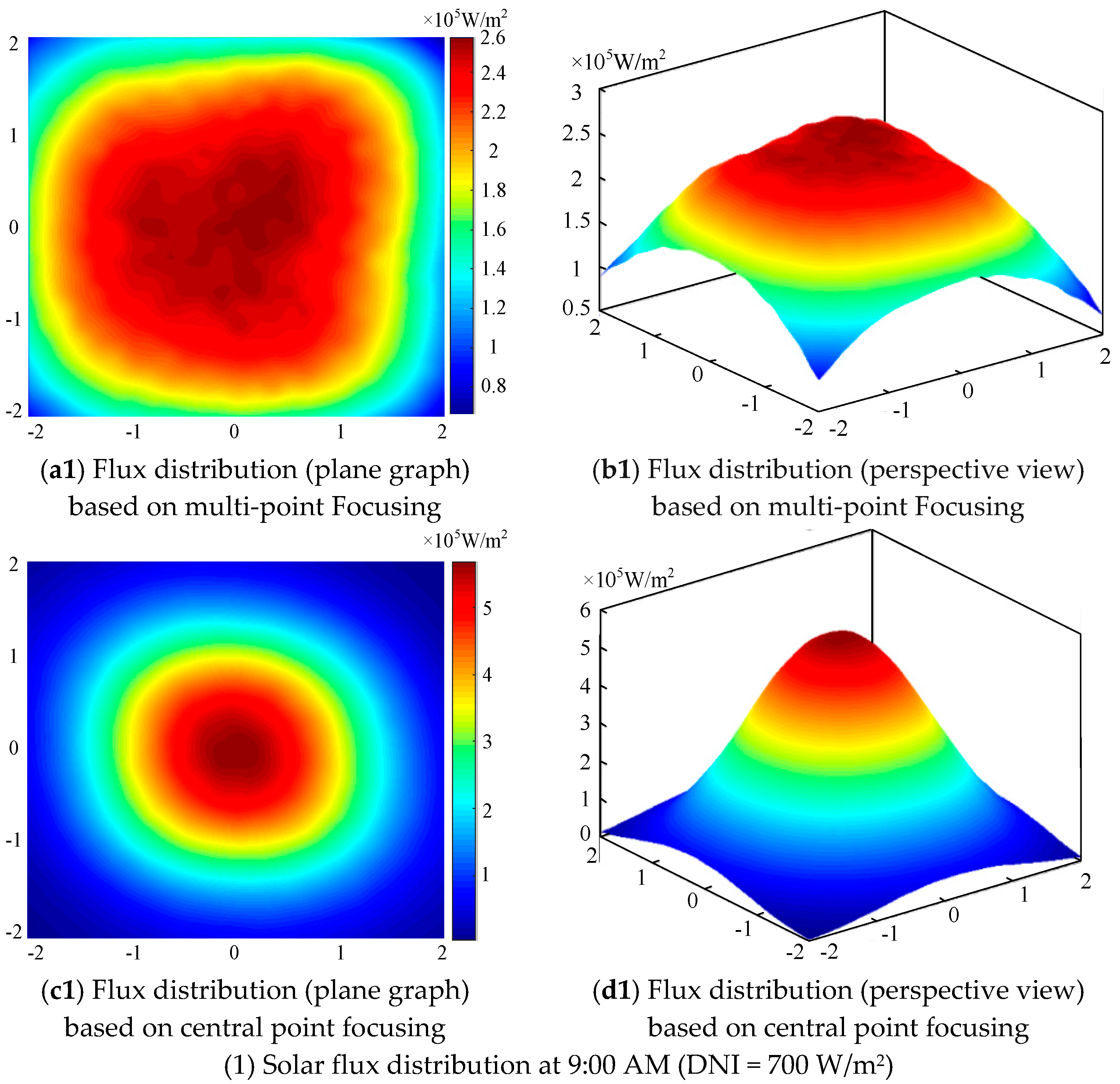
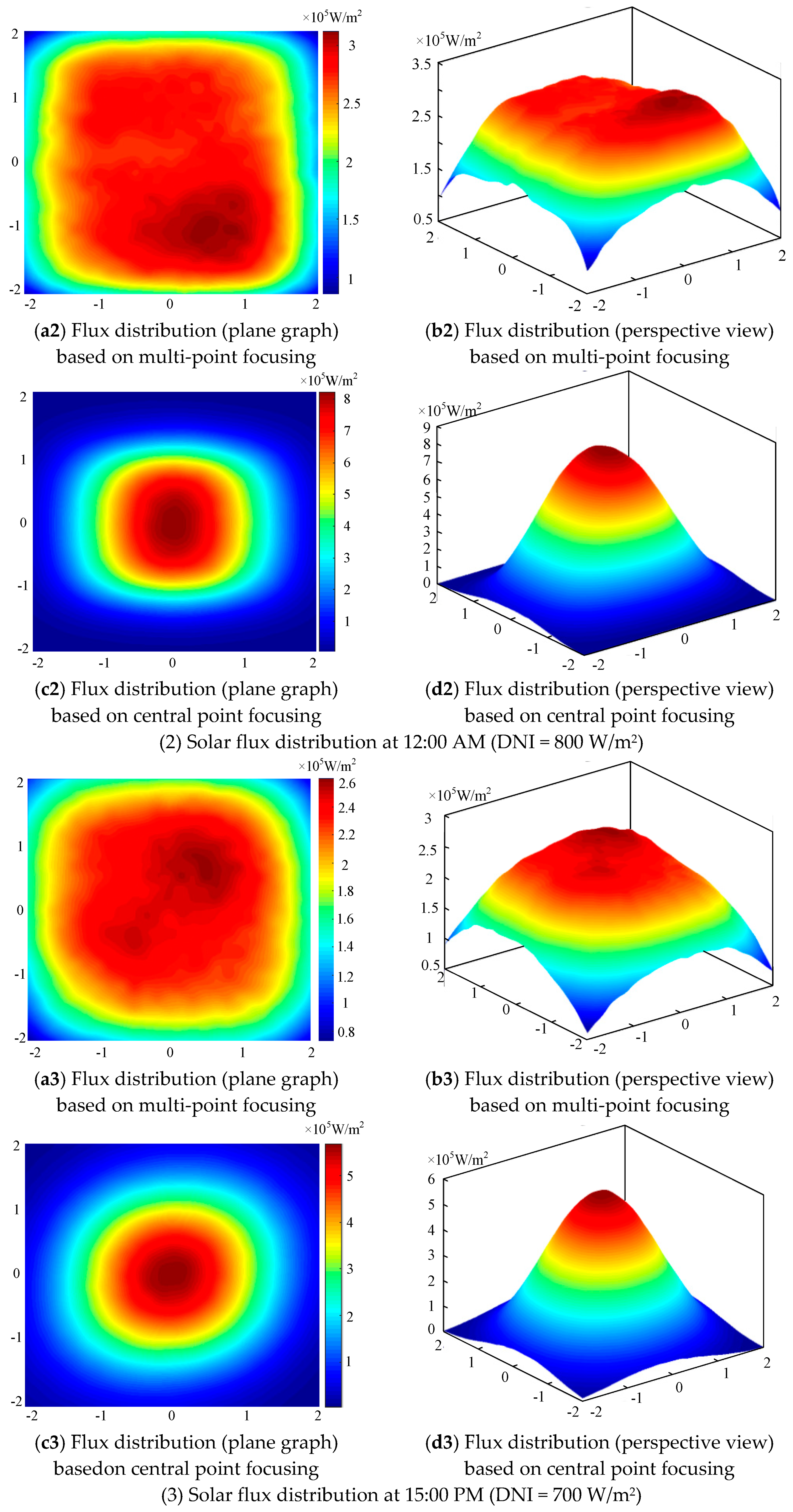
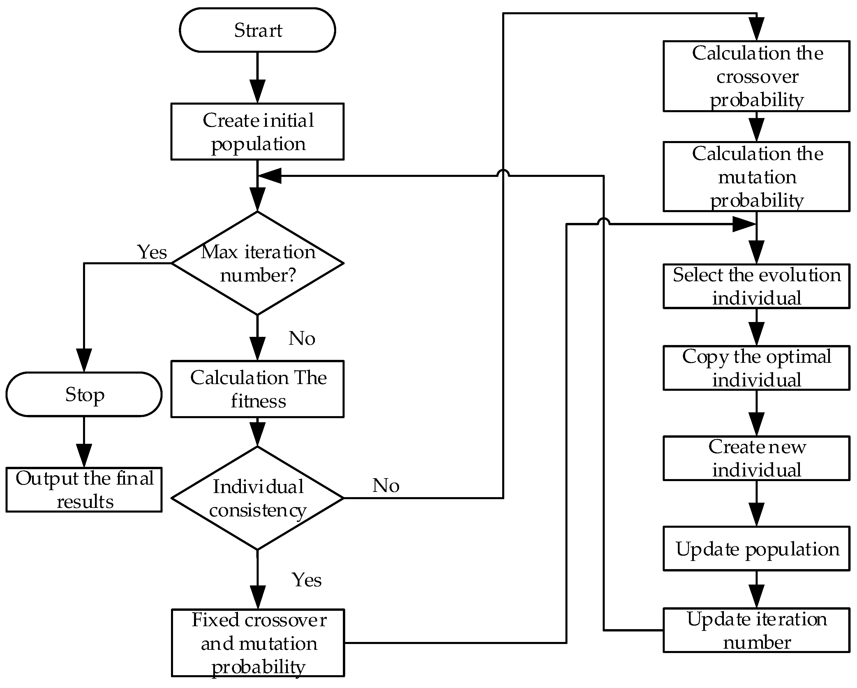
In this study, a genetic algorithm was adopted to improve the heliostat’s focusing positions on the receiver. The aim of this optimized dispatch is to make the solar flux distribution on the receiver as uniform as possible while reducing the spillage loss to the greatest possible extent. In comparison with integer optimization and other algorithms in previous literatures, a self-adaptive genetic algorithm has the advantages of rapid optimal-searching and invulnerability to local optimization; therefore, it was chosen as the solver of the optimization strategy in this paper. The results show that the peak solar flux on the receiver surface declined to half of that subjected to central point focusing after an optimization strategy. Additionally, the solar flux densities in most regions were significantly similar to each other. Through the application of optimized dispatch strategy, in addition to enhancing the system efficiency of the whole plant, the safe and steady operation of the receiver was guaranteed.

2. System Introduction of 1 MWe Solar Thermal Power Plant in Yanqing

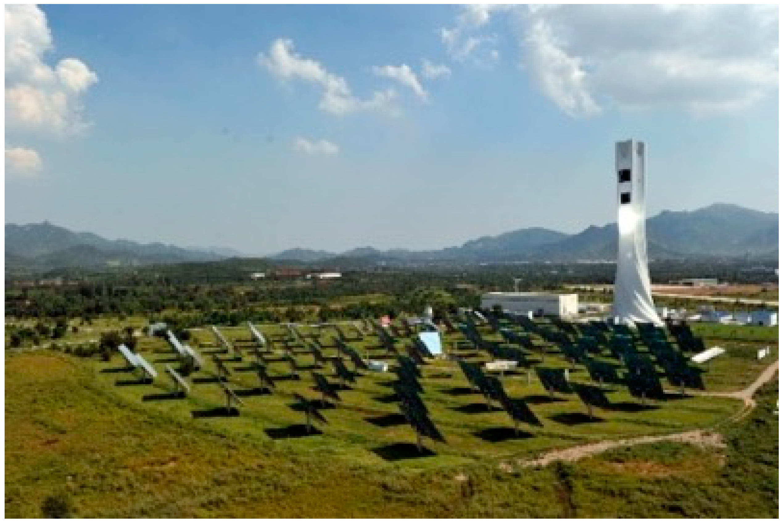
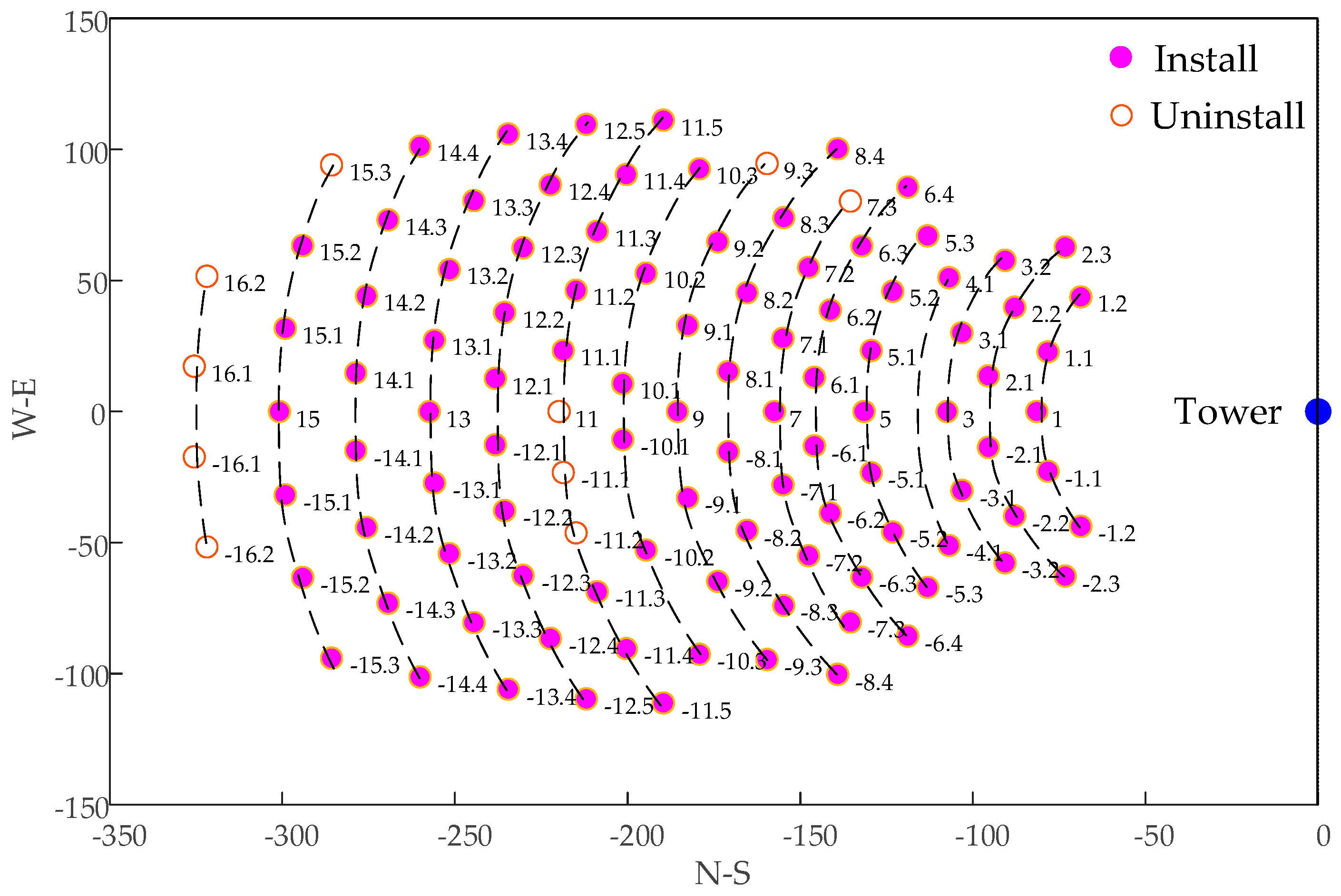
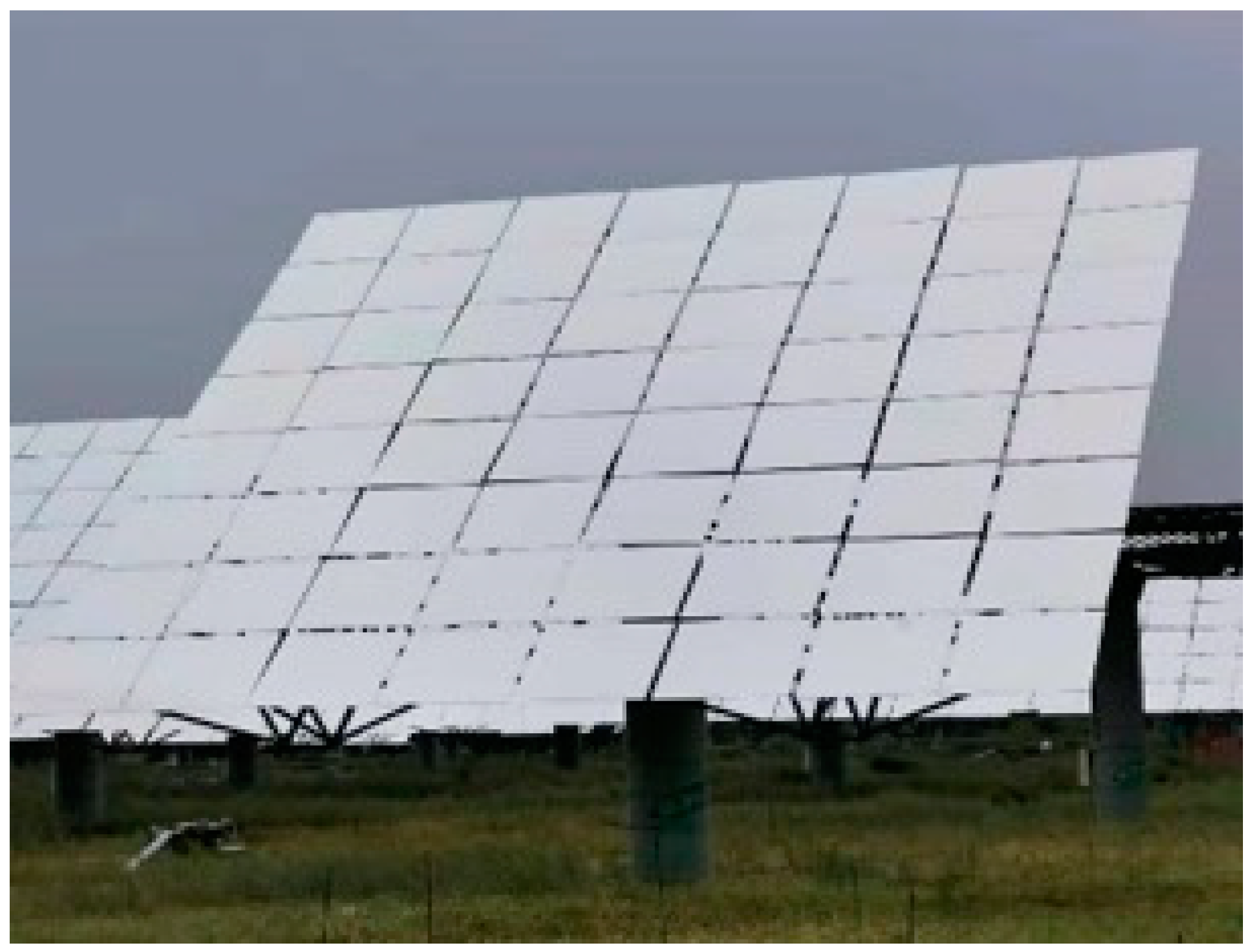
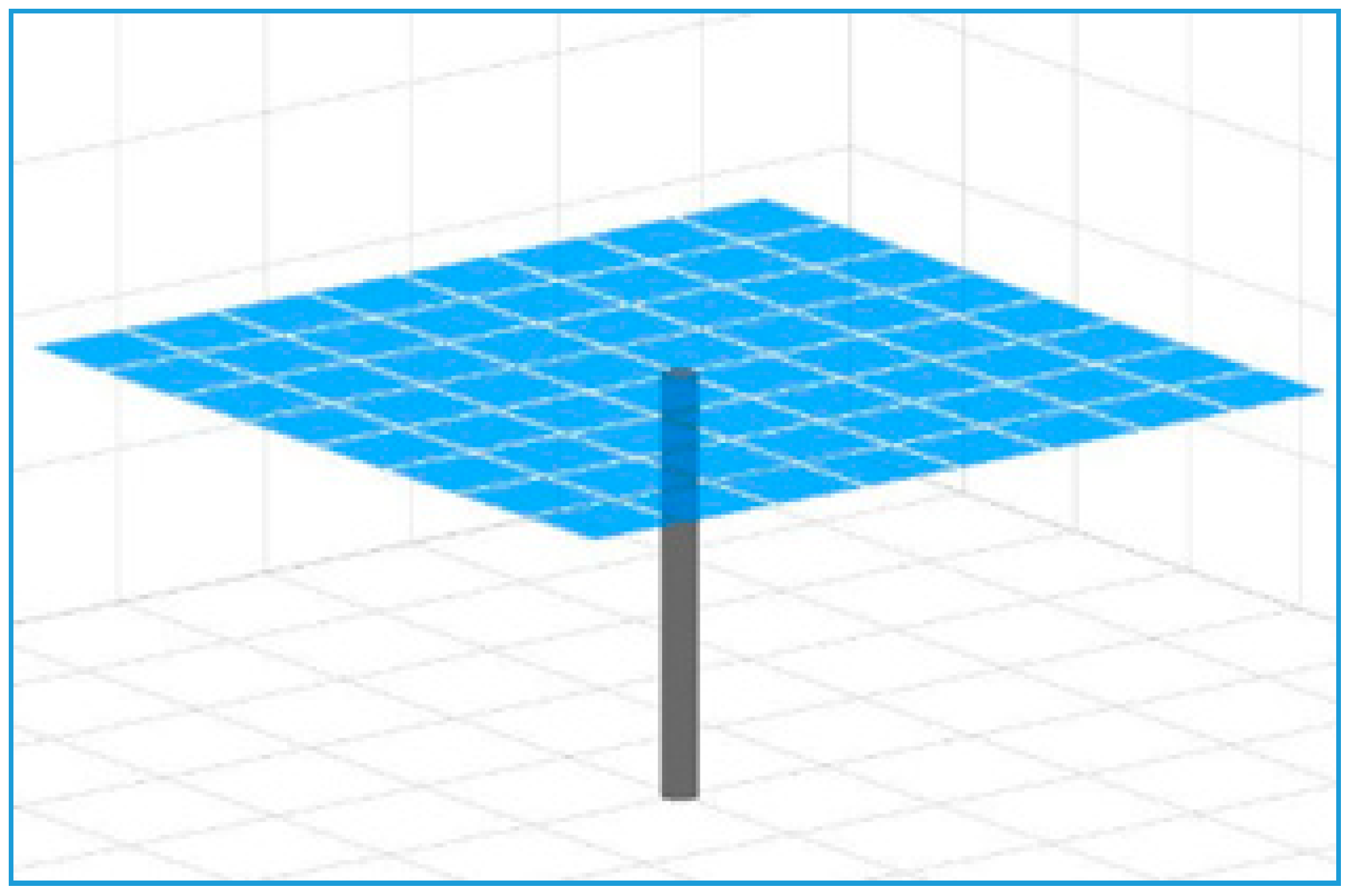
A 1 MWe CSP plant in Yanqing is the first solar thermal tower power plant at a megawatt level in Asia. This plant was constructed to study the system integration techniques for CSP tower plants [20]. It is primarily composed of a concentrating system, a receiver system, a storage system, and a power generation system. To be specific, the concentrating system is laid out in a north-south direction. Located at the north of a central tower, this system contains 100 heliostats that are in a staggered arrangement (as shown in Figure 1 and Figure 2). 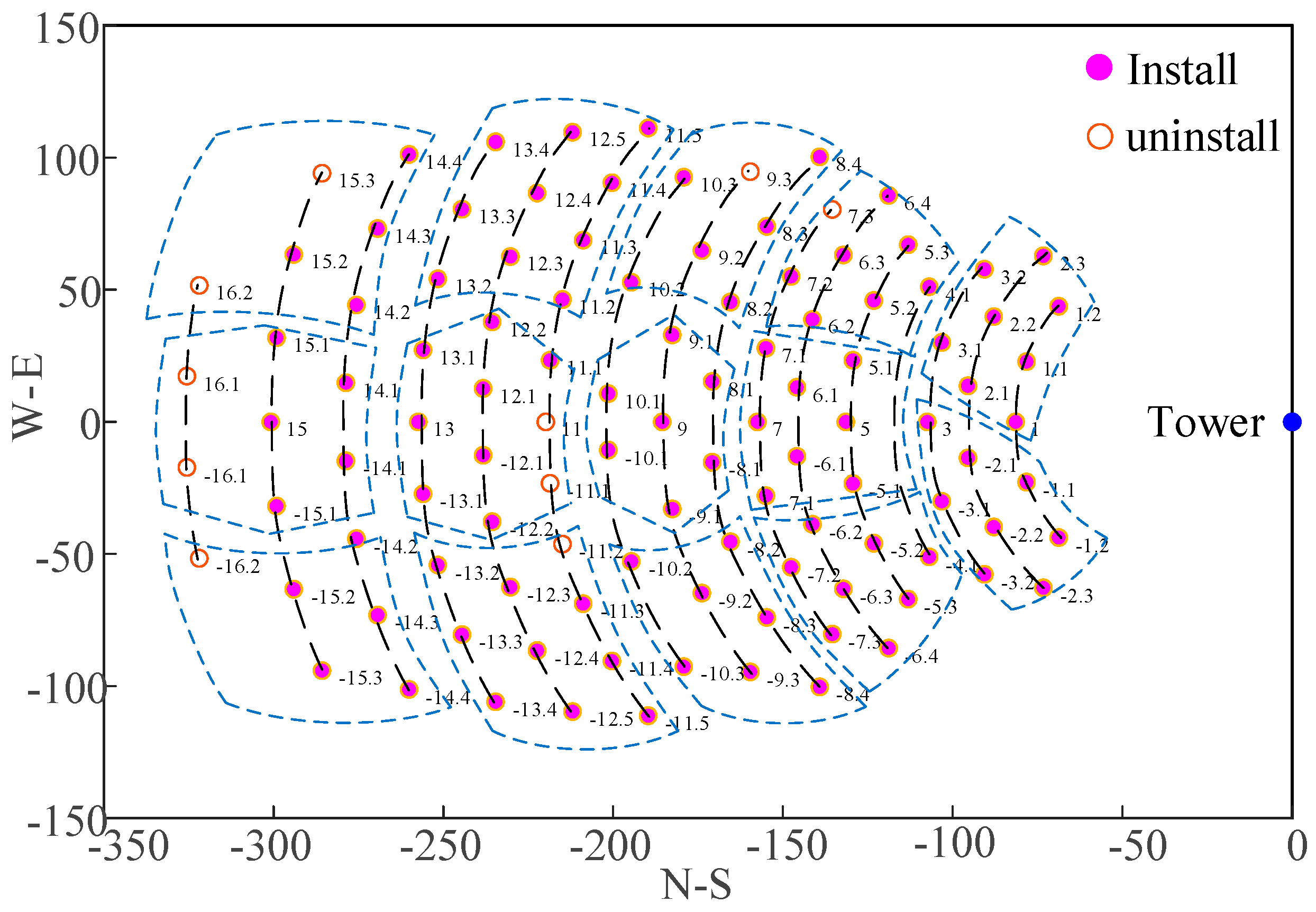Figure 1 shows a perspective view of the heliostat field in the Yanqing CSP plant, and Figure 2 is a layout drawing of the heliostat field’s coordinates in the Yanqing CSP plant. Therefore, the whole heliostat field has 15 rinds in total, and each heliostat has its own inherent coordinate. The receiver system is constituted by a cavity receiver installed at a location 78 m height from the tower. In this way, solar energy concentrated by the concentrating system can be converted into the thermal energy of the working fluid. In this study, research contents were only limited to the “concentrating-receiver” coupling system.

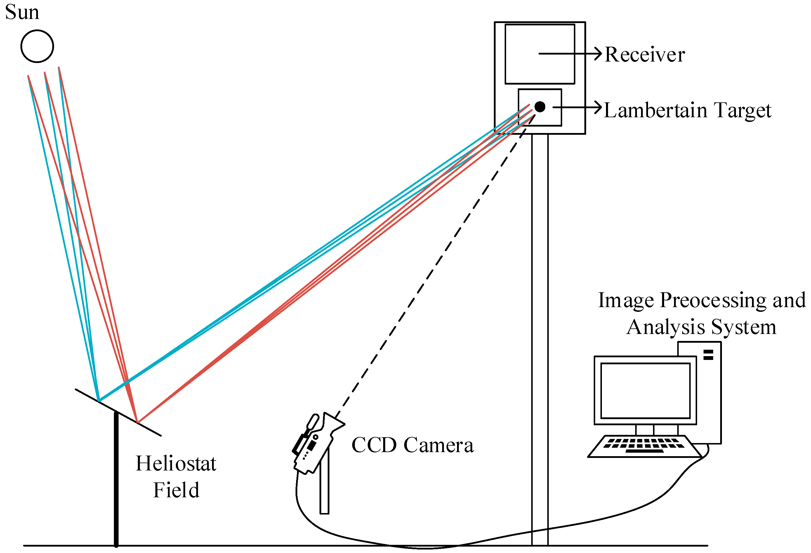
During the operation of a power plant, the control precision of a concentrating system largely affects the tracking precision of a heliostat. The control system of the heliostat field in the Yanqing CSP Plant consists of an host computer, a beam characterization system (BCS), a central control interchanger, and a lower computer. Among them, a BCS provides a technical guarantee for a heliostat to accurately focus on the receiver. It is comprised of a high-resolution industrial CCD camera (effective number of pixels 1600 × 1200, cell size 4.4 × 4.4 μm). Each pixel has eight bits or, equivalently, 256 levels. The selected lens was the Nikon^® (Nikon Corporation, Tokyo, Japan) AF-S Ø95 (zoom range: 200–500 mm, F5.6), and an image processing software and its working diagram is presented in Figure 3. The fundamental service principles of a BCS are described as follows: Based on a track angle bias strategy, the concentrating characteristics analysis system is utilized to gain the corrected values of two reference tracking axis positions of the heliostat, and the corrected values are also saved in the bias correction database [21]. During operation, the reference positions of heliostat’s azimuth and altitude axes are calculated in line with solar moving orbit. While a heliostat tracks the sun, the corrected values of reference positions for two tracking axes are incorporated to reduce the time-varying tracking errors of the heliostat. Under the action of a BCS, the heliostat’s tracking error of the Yanqing CSP plant can be controlled below 0.4 mrad. During the experiment, a white Lambert target was selected as the focal target. As a perfect diffusing surface, the Lambert target presented the same apparent brightness from any angle. This provided a theoretical basis for our experiments [22]. Once the heliostat focused on the Lambert target, a CCD camera was utilized to take photographs of solar spots (the camera was situated at a middle position of the 11th ring in the heliostat field). The acquired solar spot information, subsequent to grey processing, was converted into a percentage based chart of flux distribution. Currently, the heliostat field of this plant is mostly controlled by single-point focusing, which is located at the center of the receiver. In this case, the uneven solar flux distribution on the receiver was likely to affect the secure operation of the receiver system and shorten the service life of the receiver.

3. Modeling of Heliostat Field

In the heliostat field of the Yanqing CSP plant, each heliostat as high as 6.6 m covers an area of 100 m² (10 × 10 m). Moreover, it is formed by 64 small square plane mirrors (each 1.25 × 1.25 m) by means of stitching; this is shown in Figure 4. To explore the solar flux distribution on the receiver surface, modeling must be conducted for the entire heliostat field. The only differences in heliostats are their positions. Specific to the whole concentrating system, an individual heliostat was thus selected as the modeling object to set up a mathematical model based on the Monte Carlo ray tracing method. Since there has been much research which has adopted the Monte Carlo method for the modeling of a heliostat field by previous scholars [23,24], the detailed modeling process is not elaborated here. In this study, only investigations that are different from those of former researchers are described. In preceding literature, heliostat modeling has assumed the reflector as an ideal continuous curved surface in most cases, or the direct fitting of solar flux distribution is fulfilled on the receiver in accordance with the law of Gaussian distribution. Additionally, not only does a tilted angle error exist when the plane mirror approaches the curved surface, the influence of heliostat support structure on solar flux distribution has hardly been considered by preceding scholars in the course of modeling. To carry out concentrating system modeling in this paper, both the stitching structures of the actual curved surface and the gaps of individual plane mirrors were taken into account. Meanwhile, it was assumed that heliostat errors complied with normal distribution. A schematic diagram of the heliostat model is presented in Figure 5.

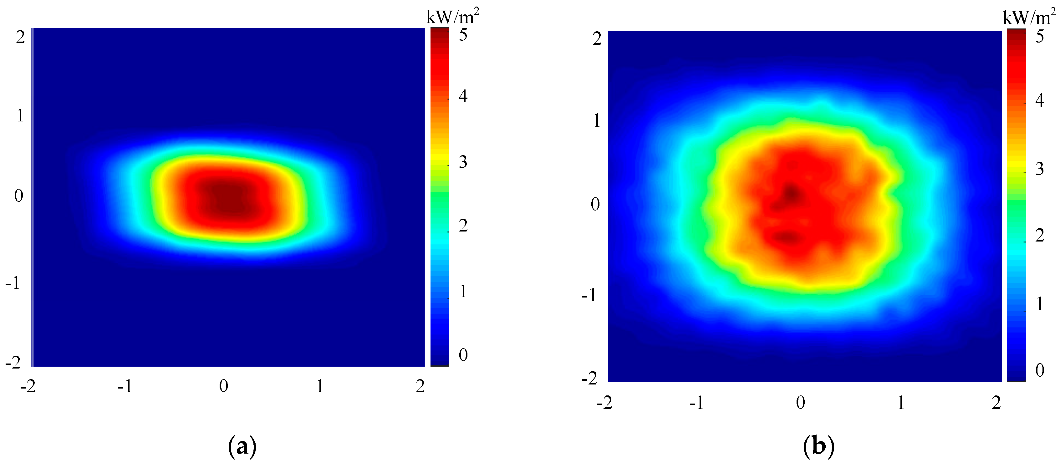
To study the effects of different mirror surface processing modes on solar flux distribution during modeling, a heliostat with coordinates of #8.1 was randomly selected to carry out the simulation of solar flux at noon of the vernal equinox day. Such simulation was targeted at both the ideal and the actual mirror surfaces, and the simulation results are given in Figure 6.

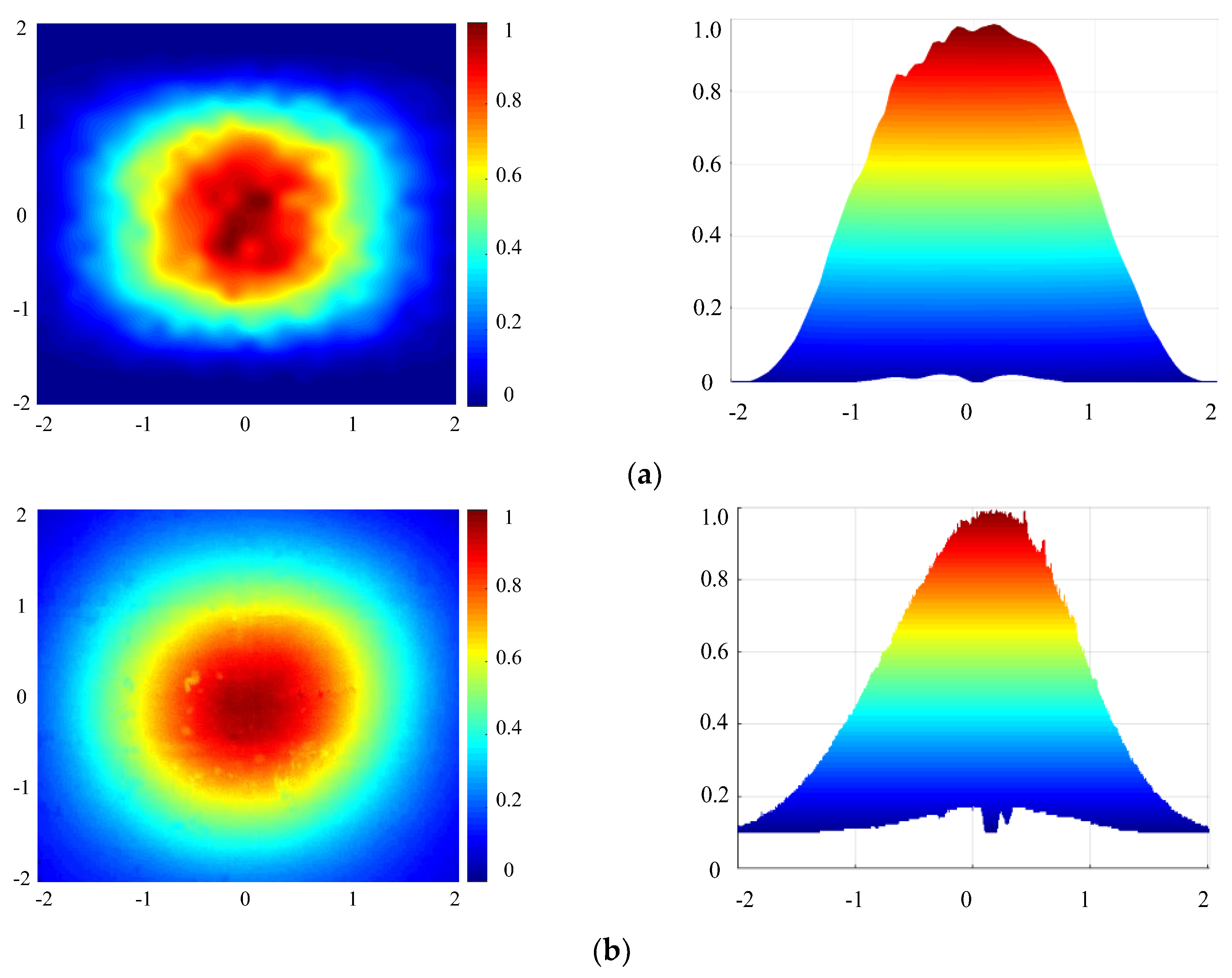
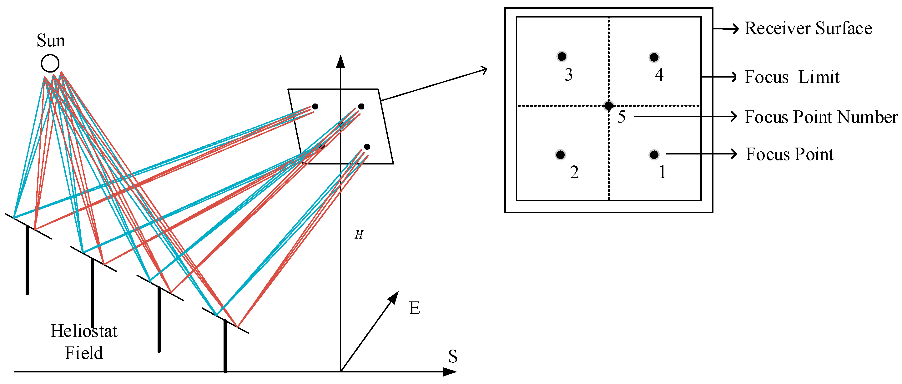
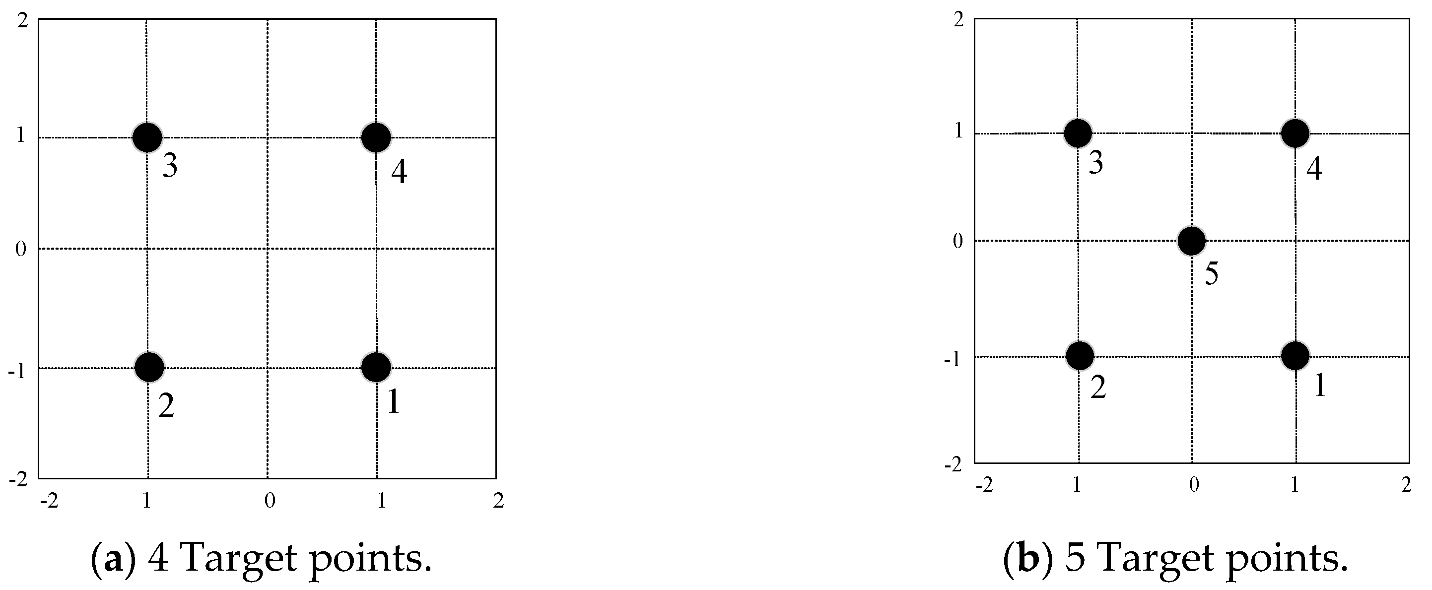
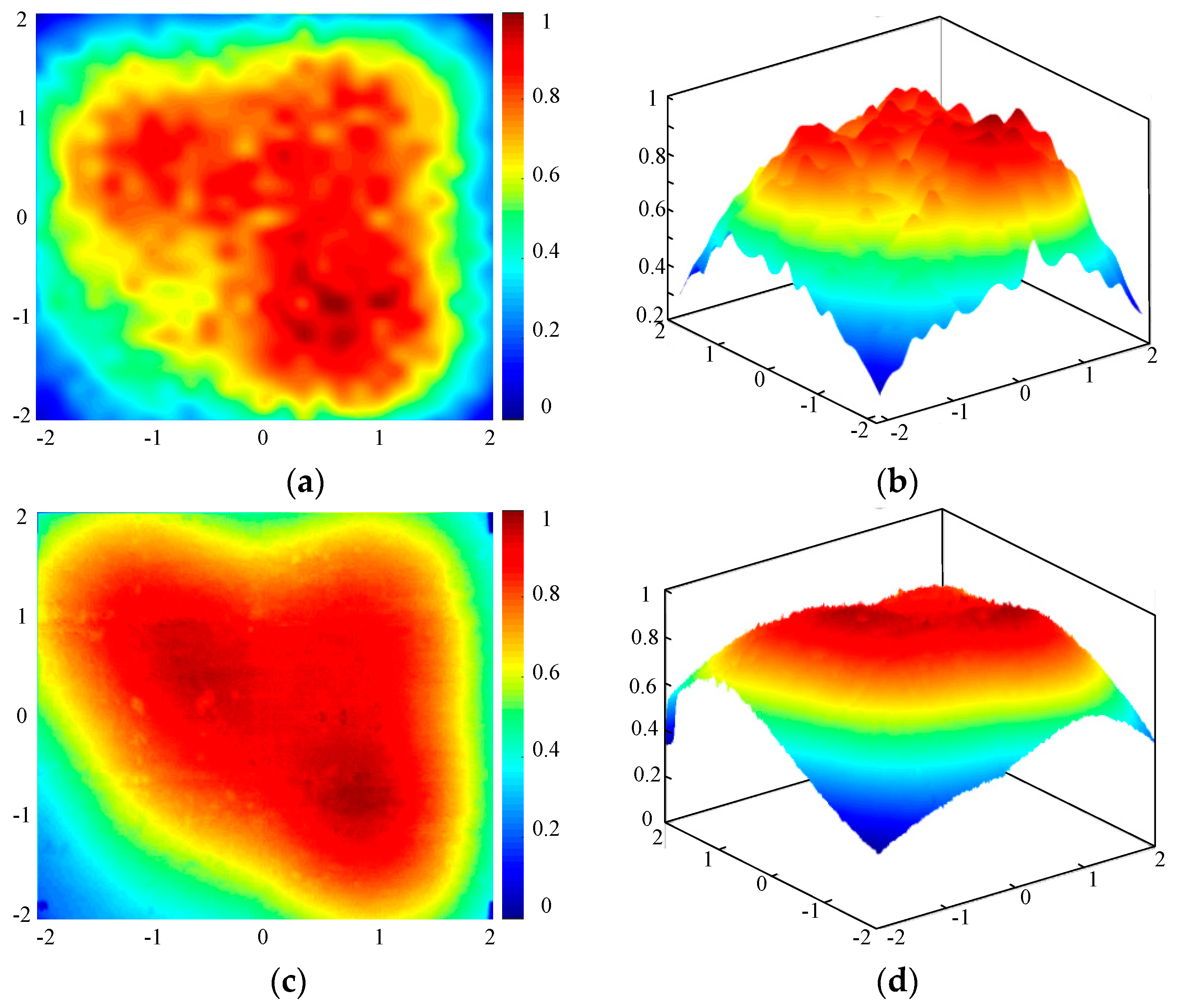
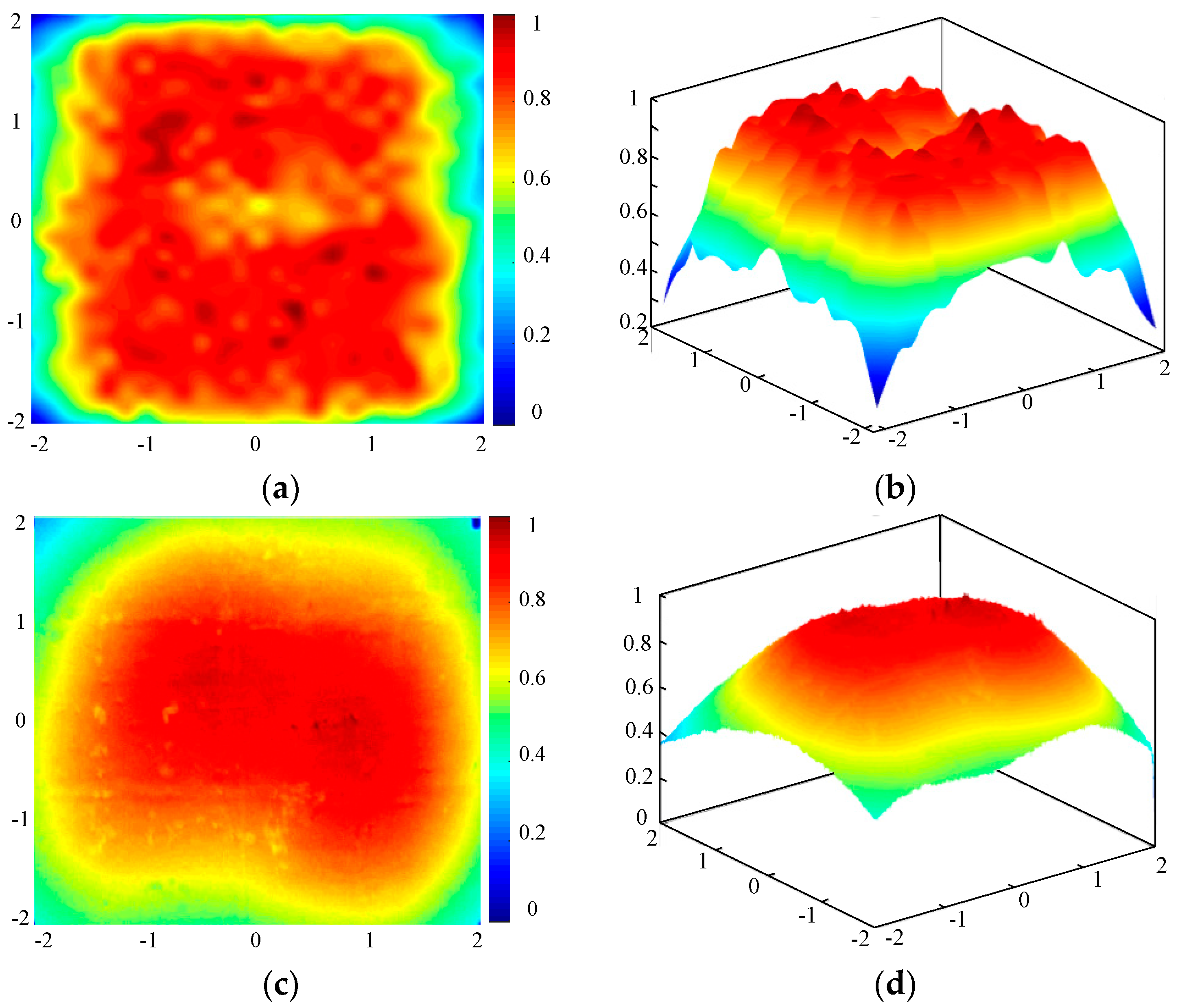
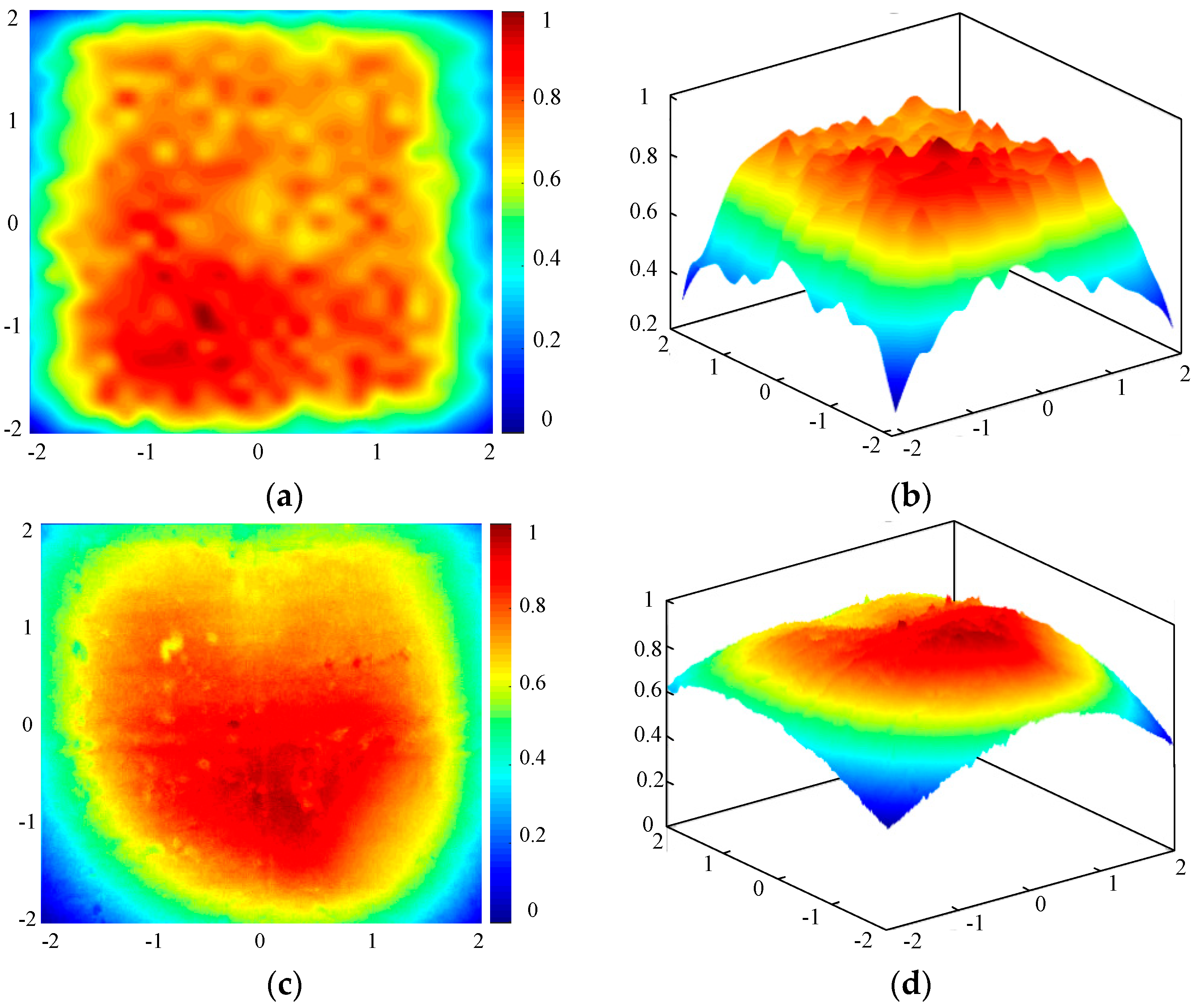
As shown in this figure, it can be clearly observed that the solar flux distribution of the ideal mirror surface on the receiver perfectly conformed to the Gaussian distribution, which was embodied in regular shapes and small spot diameters. In regard to the spliced mirror surface, although the solar flux distribution of its focus spot presented a Gaussian distribution on the whole, peak energy could be found in local areas. Additionally, the shape of solar spot was relatively large. To verify the validity of the established model, the focusing points of the #8.1 heliostat were set at No. 4 and No. 5 (the set of focusing points is shown in Section 4.1 in this paper) at noon on 4 September 2019 (clear weather). The comparison results between simulation and experiment were given in Figure 7 and Figure 8. To better perform the comparative analysis, the solar flux distribution was normalized.

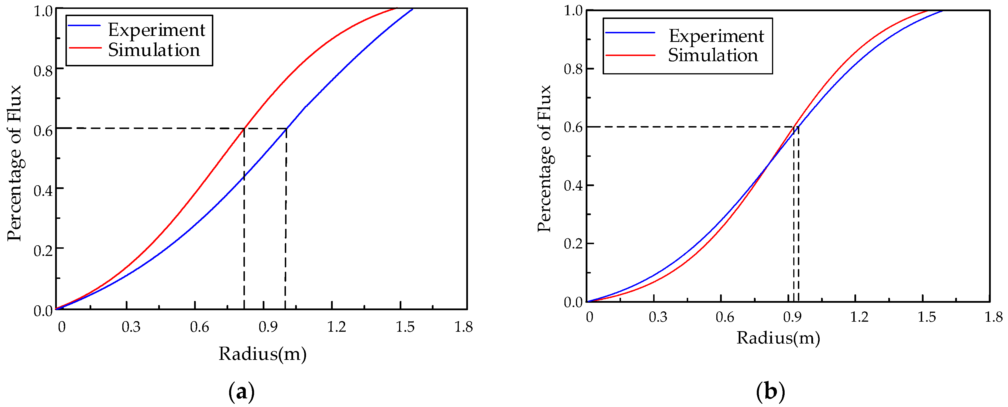
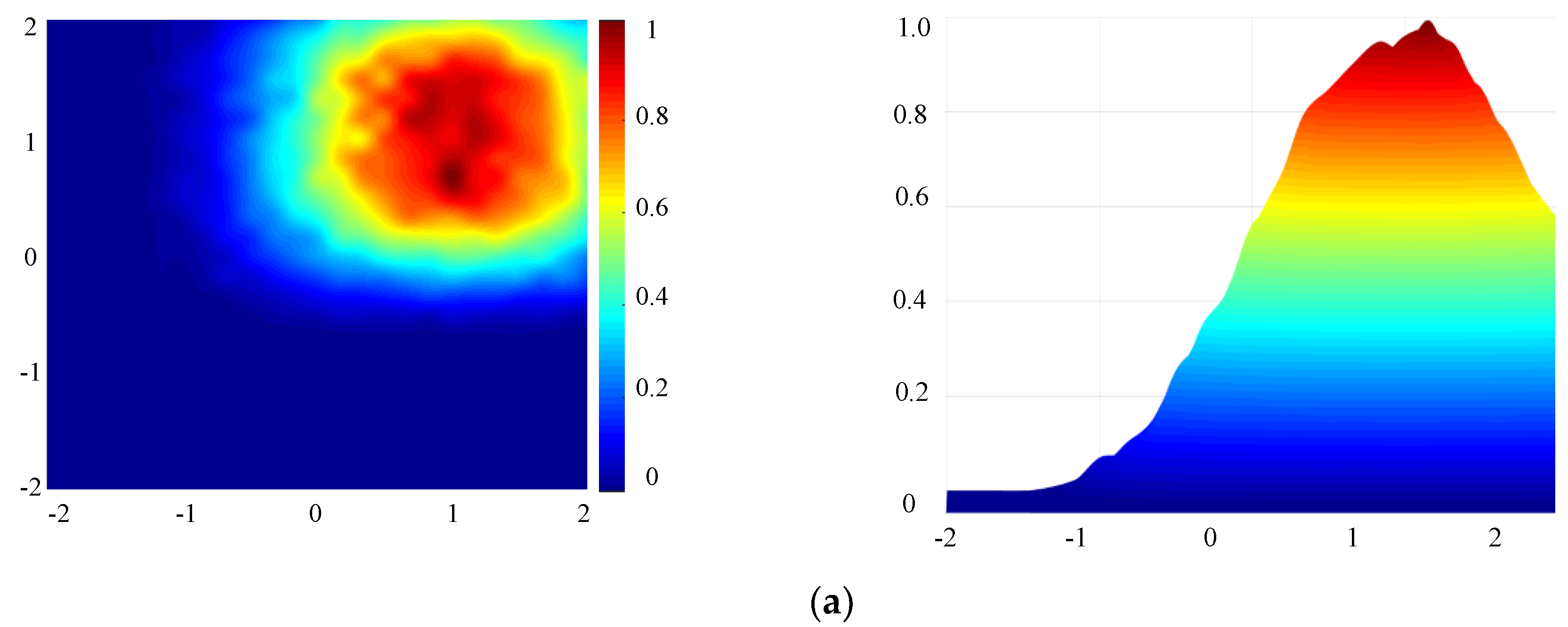
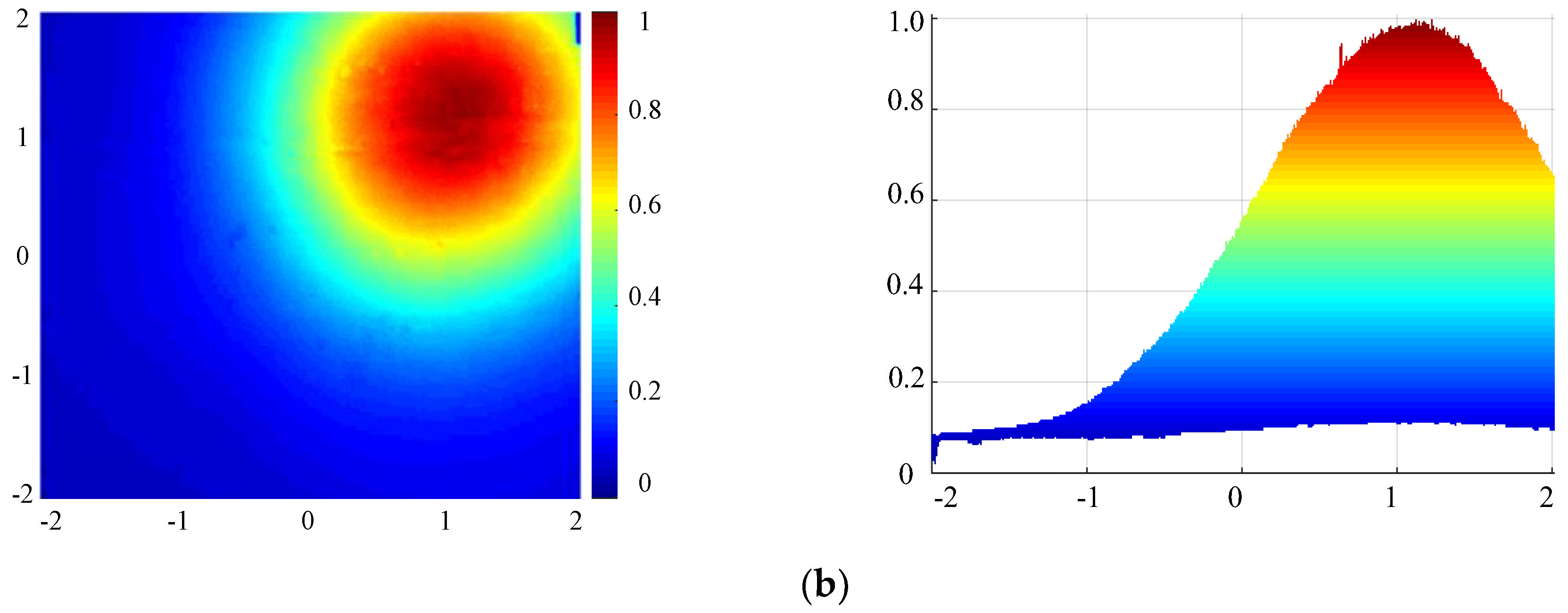
To observe solar spot similarities in a more intuitive manner, a curve chart (as shown in Figure 9) was portrayed according to the information presented in Figure 7 and Figure 8; thus, variations in proportions taken by the spot energy and their radius could be clearly presented.

Figure 9a presents the variation trend of the energy percentage as the spot radius changed when the heliostat focused on the #5 focal point. To be specific, the solar spot radius of the simulation and the experiment were, respectively, 1.48 and 1.55 m. In this case, the relative error was less than 4.8%. Moreover, the radii of the simulation and experimental focus spot containing 60% energy were 0.87 and 0.98 m, respectively, and the difference seemed very small. Figure 9b shows the relation curve when heliostat focused on the #4 focal point. Here, the simulated and experimental spot radii were 1.53 and 1.58 m, respectively, and the relative error was less than 3.2%. Different from Figure 9a, the simulation and experimental radii for areas containing 60% of the spot energy turned out to be 0.91 and 0.93 m, respectively, and the difference was only 0.02 m, which is fully acceptable.

As shown in these figures above, it is noted that the solar flux distribution of simulated solar spot was rather close to experimental result. Moreover, the spot sizes also agreed well with the experimental data. According to comparison results, the spliced curved surface could reflect the actual effect of the heliostat better, which verified the validity of the model established here.

4. Optimized Dispatch Design for the Heliostat Field

4.1. Target Point Settings for Concentration

In theory, any point on a receiver can be seen as a focal point during the optimized dispatch of a heliostat field. Mathematically, however, the distribution of focal points is a non-linear continuous optimization problem, which means that the focusing situations of a heliostat field may become complex beyond example. If a heliostat only focuses on several target points, the optimized dispatch of a heliostat field is deemed as a target assignment optimization issue. In this case, the continuous optimization problem turned into a discrete problem that was associated with target assignment. Additionally, the complexity of the solution space was also substantially lowered. Therefore, provided that both quantities and locations of focal points on the receiver are confirmed, a focusing strategy optimization model can be established for a heliostat field. Here, the solar flux distribution of the receiver’s opening surface was adopted as the research object, and the actual spot sizes and the intercept efficiency were selected to define the focal point locations. Hence, the following selecting criteria were formulated. Based on these criteria, a schematic diagram for a heliostat’s concentrating process and focal point selecting is presented in Figure 10.

(1)

The edges of the receiver should be avoided to reduce the spillage of the solar spot.

(2)

The distance between two adjacent focal points should be no less than the minimum distance that plays a role in distinguishing the spot centers of heliostats in diverse regions.

(3)

The center of the receiver surface should be selected as its focal point.

Regarding the selection of focal points, it should be noted that the distance between adjacent focal points should be determined by spot size. As seen in the comparative analysis shown in Figure 9, the radius of a spot containing 60% of the energy was about 1 m. During focusing, adjacent focal points should be firstly capable of differentiating the centers of various spots. Secondly, within a region where the spots overlap with each other, solar flux density is close to the peak solar flux of an individual solar spot. In other words, the part where the spot energy is below 50% should fall into the category of an overlap area. Therefore, the optimal gap of focal points is defined at 2 m in this paper.

In the context of multi-points focusing of a heliostat, the most important factor that affects the solar flux distribution on a receiver is the tracking precision of heliostats. Under the actions of a mechanical error and the external environment, a tracking error is necessarily inherent in the heliostat. This enables the central point of the focusing spot to deviate from the actual focusing point. In the heliostat field, a heliostat that is most far away from the receiver is located at the 15th ring, and the distance from this heliostat to the receiver is 270 m. In this case, the maximum offset between the actual central position of the heliostat’s focusing point on the receiver and the target point was 0.1 m. The least distance was 79 m, and an offset of the spot center was 0.05 m. With regard to the distances of focal points, the spot center offset led to a rather low distribution error of solar flux. For this reason, the influence caused by the tracking error may have been neglected during analysis. During the multi-points experiment, the center of the focus point was deemed to coincide with the target point.

4.2. Heliostat Regionalization Methods

In a commercialized CSP plant, a heliostat field is large and contains thousands of heliostats. During operation, the actual manipulations may be rather complicated, and the implementation cost can be even higher if their focal points are controlled one by one. In order to better serve the actual power plants, dividing the heliostat field into several groups is considered to be a comparatively economical, highly feasible, and effective method according to the similar characteristics of their focused spots. For this purpose, a novel heliostat grouping approach was proposed for this paper. By regarding heliostats’ contribution degrees and the incidence cosine similarity as grouping standards, the entire heliostat field was divided into multiple sub-regions. Here, two groups of heliostats in the symmetrical position (#9.2 vs. #−9.2 and #8.2 vs. #−8.2 in Figure 2) were randomly selected to study the incidence cosines on the vernal equinox day. The corresponding comparison results are given in Figure 11.

Apparently, incidence cosines of adjacent heliostats (#9.2 vs. #8.2 or #−9.2 vs. #−8.2) had an identical variation tendency. Within the same ring, the symmetrical heliostats (e.g., #9.2 vs. #−9.2 or #8.2 vs. #−8.2) had significantly different incidence cosines in a day. For example, the incidence cosine of heliostats in the east (#9.2 and #8.2) reached its maximal value at 1:00 PM, while the maximum incidence cosine of heliostats in the west (#−9.2 and #−8.2) was generated at 11:00 AM. This means that the heliostats in different locations contributed different energies to the receiver under the same solar radiation. Based on the above analysis, the grouping method of the heliostat field should abide by the following fundamental principles:

(1)

The number of heliostats in a group should be similar to that in another group.

(2)

Heliostats in the same group should not be excessively distant from each other.

(a)

Spot shapes reflected by heliostats close to each other are similar, and no great discrepancies exist in their solar flux distribution.

(b)

Their incidence cosines are similar, and no great discrepancies exist in the total energy provided by each heliostat.

On account of the above principles, the heliostat field in the Yanqing CSP plant was divided into 14 sub-regions, and the result is shown in Figure 12. During focusing, heliostats in the same group focused on the same target point as a whole.

4.3. Optimization Goal Settings

Once the number of target focal points and the size of heliostat field sub-regions were defined, the optimized dispatch of a heliostat field became a discrete optimization combination problem in a confined space. As a result, the complexity of the solution space greatly dropped. The sample space of heliostat field optimization is expressed in Equation (1):

$$\max =T^h$$

(1)

where $T$ refers to the number of target points and $h$ refers to that of the sub-regions in the heliostat field.

The so-called optimal focusing strategy of a heliostat field should be formulated from two perspectives. One is the safety of the receiver, and the other is the energy collected by receiver. On the premise of ensuring the receiver’s safety, the solar flux densities on the receiver should be uniformly distributed to the greatest extent. At the same time, the spillage loss of the solar spot should be minimized. A mathematical expression for optimization goals and boundary constraint conditions of the model is given below:

$$\{\begin{array}{l}\min \delta \\ F\le F_0\\ {\eta }_{\mathrm{int}}\le 15\%\end{array}$$

(2)

In Equation (2), $\delta$ stands for a standard deviation of solar flux density, $F$ is the actual average solar flux density on the receiver, $F_0$ is the maximum solar flux density that is allowed by the receiver, and ${\eta }_{\mathrm{int}}$ is the spillage loss of receiver. Moreover, both the optimization goal and the constraint condition are established to meet solar flux distribution and receiver safety requirements.

4.4. Optimization Algorithms

Nowadays, many algorithms have been applied in heliostat field optimization, including the heuristic tabu method [10], mixed-integer programming [11], the greedy algorithm [25], the genetic algorithm (GA) [8] and particle swarm optimization (PSO) [19]. Here, the GA was selected as a solver of relevant problems. Historically, the GA is a stochastic algorithm derived by professor Holland from the law of nature known as “it is not the strongest of the species that survive, but the one most responsive to change” proposed by Darwin [26]. Among stochastic optimization algorithms, the GA is the most widely applied approach. The basic thought of this algorithm is to simulate biological evolutionism and genetic mechanism and, thus, see an optimization process as a natural evolutionary process. In this manner, an optimal solution [27] can be found. During iterative optimization, the GA starts with population of problem solutions to search, instead of individual solutions to the problem like other optimization algorithms. Considering this, it has a wide coverage and benefits to global optimization. Additionally, the corresponding solving process is independent of information related to search space. On the contrary, only fitness function values are used to evaluate individuals and implement genetic manipulations. Moreover, the GA may undergo self-optimization during iteration, indicating that such an algorithm has the features of self-adaptability and self-learning [28]. Concerning the optimization problems in this study, the solar flux distribution on the receiver cannot be accurately expressed by a mathematical equation. In addition, the solar spot formed by a single heliostat is also a discrete datum. Therefore, the traditional optimization algorithm based on calculus theory could be applied to this situation, as it also requires that the objective function in the optimization problem to be differentiable or at least continuous. Though the heliostat grouping method and database were designed to reduce the running time of the optimization program in this study, an efficient search program was still needed to completed the optimization strategy in the relatively shorter control period of a heliostat field. In search algorithms, a traversal method is usually used to find the optimal solution of the target in the process of searching, such as the meta-heuristic and particle swarm optimization. As a result, the calculation process takes a long time, which did not meet the application requirements of this study. In contrast, the genetic algorithm has great advantages in search speed by means of population evolution, and it can search for multiple possible optimal solutions in one iteration. At the same time, it has a low requirement for the mathematical analytical properties of the optimization objective, and it is especially suitable for the optimization of discrete problems. In such case, it is rather appropriate to solve these problems by means of the genetic algorithm.

In regard to the application to heliostat fields, at the very beginning of the iteration, a random target point should be confirmed for each group of heliostats. Alternatively, no target points may be defined—that is, no focused spot on the receiver. On the corresponding focus point, the spot information of heliostats was retrieved from a database in consistency with the confirmed target point. Then, fitness was figured out for every individual in the population of solutions, and an individual with the lowest fitness was removed. As for elite individuals in the retained population, they were directly reproduced to a new-generation population and also selected as evolved individuals. Hence, crossover and mutation operations could be executed to further generate a new generation of individuals that could be incorporated in the population. During the successive population update, new individuals produced from the new-generation population were able to evolve to those of higher fitness. For the purpose of ensuring convergence to a globally optimal solution, the probabilities of both crossover and mutation may have automatically varied during optimization based on fitness values. In this way, the diversity of population is maintained and locally optimal solutions could be avoided. Computational formulas for crossover probability $p_c$ and mutation probability $p_m$ are given below.

$$p_c=\{\begin{array}{c}\frac{p_{c1}(f_{\max }-f_c)}{f_{\max }-f_{avg}}\hspace{1em}{f}_c\ge f_{avg}\\ p_{c2}\hspace{1em}{f}_c<f_{avg}\end{array}$$

(3)

$$p_m=\{\begin{array}{c}\frac{p_{m1}(f_{\max }-f_m)}{f_{\max }-f_{avg}}\hspace{1em}{f}_m\ge f_{avg}\\ p_{m2}\hspace{1em}{f}_m<f_{avg}\end{array}$$

(4)

where $f_{\max }$ and $f_{avg}$, respectively, represent the maximum fitness and the average fitness of population; $f_c$ is the higher fitness among two individuals on which crossover is performed; $f_m$ is fitness of individuals subjecting to mutations; $p_{c1}$, $p_{c2}$, $p_{m1}$ and $p_{m2}\in [0,1]$, with $p_{c1}<p_{c2}$ and $p_{m1}<p_{m2}$. In this context, a fitness function can be expressed in the following Equation (5).

$$f=\delta$$

(5)

Upon the termination of the algorithm, an optimal individual was acquired, and it was the optimal focusing strategy of the current heliostat field. On this basis, the respective focus points of subregions in the heliostat field were determined. Under the premise of ensuring receiver safety, such a focusing strategy has the capability to make solar flux densities that are uniformly distributed on the receiver. A flow chart of optimization is presented in Figure 13.

5. Results and Discussions

5.1. Optimization Strategy Verification

To verify the thought that the proposed optimized dispatch strategy could realize uniform flux distribution on the receiver and check both validity and uniqueness of such a strategy, two groups of focal points in different quantities were designed on a 4 × 4 m receiver surface, as shown in Figure 14. Their biggest difference lied in the addition of a central point of the receiver.

The distribution and quantity of focal points on the receiver exert significant influences on optimization space. Under the circumstance that the number of heliostats remains unchanged, one more focal point corresponds to a multiple growth of solution space, which is expressed in Equation (6). This dramatically increases the calculated amount of optimization.

$$M=\frac{{(T+1)}^h}{T^h}$$

(6)

According to focal point distribution in Figure 14, the #−4.1, #5.1, #6.2 and #8.1 heliostats (see Figure 12) in the heliostat field were randomly selected to perform a simulation study. As the heliostat field was regionalized above, the selected heliostats were located at different sub-regions and distributed on the eastern and western sides of the heliostat field. At different times on the vernal equinox day, both the quantity and positions of focal points focused on the receiver after an optimized dispatch was obtained. For details, please see

Table 1. Focus positions of heliostats (four or five focal points).

	Focal Point	No. 1	No. 2	No. 3	No. 4	No. 5
Time
9:00 AM		#5.1/#5.1	#−4.1/#−4.1	#8.1/#8.1	#6.2/#6.2	NO/NO
12:00 AM		#5.1/#5.1	#−4.1/#−4.1	#6.2/#6.2	#8.1/#8.1	NO/NO
15:00 PM		#8.1/#8.1	#−4.1/#−4.1	#6.2/#6.2	#5.1/#5.1	NO/NO

.

It can be observed from Table 1 that distribution optimization results of the two groups of focal points were completely identical at different times on the vernal equinox day. In other words, the addition of the central point did not lead to a change in the optimization result. This means that the optimization algorithm has the potential to not only effectively define the positions of focal points for heliostats but also make solar flux densities uniformly distributed on the receiver. Meanwhile, the uniqueness of solutions acquired through such an algorithm was also validated.

In order to verify the feasibility and validity of optimization results, the above four heliostats were selected to perform experimental verification at different times on 4 September. The focal point positions after optimized dispatch is shown in

Table 2. Focal points of heliostats at different times on 4 September.

	Focal Point	No. 1	No. 2	No. 3	No. 4
Time
9:00 AM		#5.1	#−4.1	#8.1	#6.2
12:00 AM		#5.1	#−4.1	#6.2	#8.1
15:00 PM		#8.1	#−4.1	#5.1	#6.2

.

During the experiment, the heliostat focal points were set as corresponding coordinates according to their positions at different times, as presented in Table 2. The solar flux distribution on the receiver surface at diverse moments are reflected in Figure 15, Figure 16 and Figure 17.

In Figure 15, the solar flux densities of the No. 2 focal point can be seen to be significantly lower than those in another sub-region. The major reason for this was that the sun in the morning was closer to the east, and the solar altitude was accordingly smaller. The No. 2 focal point was formed by the #−4.1 heliostat at the westernmost periphery of the heliostat field. Subjected to such an external condition, the incidence cosine loss of the heliostat was the largest, and the energy that it contributed to the receiver was comparatively less. Consequently, the solar flux density at such a focal point was below that of other focal points. As shown in Figure 16, the sun was due south at 12:00 at noon, and the solar altitude reached its highest level at the same time. Clearly, heliostat positions in the heliostat field placed the least influence on spot formation, and the heliostats provided the receiver with balanced energy. Therefore, the most uniform flux distribution phenomenon could be found on the receiver at high noon. The case shown in Figure 17 was just opposite to that revealed in the morning. In the afternoon when the sun moved toward the west, the energy provided by heliostats in the west of the heliostat field was greater than that in other sub-regions. Hence, the solar flux density of the No. 2 focal point at 3:00 PM was above that of remaining focal points.

As shown in Figure 15, Figure 16 and Figure 17, there were slight differences between the simulation and experimental results on the plane graph. The reasons are as follows: First, the existence of the tracking error of the heliostat caused the center deviation of the focused solar spot from the actual focal point. Secondly, the slight surface error resulted in a difference in the spot shape. However, it seems that the difference was relatively acceptable.

Through analysis, it could be found that, at different times selected in the morning, noon and the afternoon in a day, the experimental and simulation results of solar flux distribution on the receiver surface are generally coincided with each other. This indicates that the optimization algorithm was capable of producing an optimal dispatch strategy at any time throughout the day, which got rid of temporal influence.

5.2. Analysis of the Whole Heliostat Field

The above analysis proves the validity of the heliostat model and its optimized dispatch model from multiple perspectives. However, the number of heliostats and quantities of their target points in practical applications are far greater than those defined for the experiments. Below, the heliostat field as our research object in the Yanqing CSP plant was divided into 14 sub-regions as discussed in Section 4.2. In addition, multi-point focusing and central point focusing were employed to simulatively investigate solar flux distribution on a receiver in different periods on 4 September 2019. Corresponding results are presented in Figure 18. The heliostat count corresponding to each focal point after the optimized dispatch was conducted for sub-regions, and the result is shown in

Table 3. The number of heliostats corresponding to focal points based on multi-point focusing after heliostat field regionalization.

	Focal Point	No. 1	No. 2	No. 3	No. 4	No. 5
Time
9:00 AM		3	4	4	3	0
12:00 AM		4	3	4	3	0
15:00 PM		4	2	5	3	0

. There were different quantities of heliostats on each focal point in different time periods. This means the focusing position of heliostats may also change in a day, as the position of the sun and Direct Normal Irradiance (DNI) both change all day long.

As can be clearly observed from Table 3, no group focused on the central point (the No. 5 focal point) when multi-point focusing was adopted due to the two following major aspects. First, the solar spots of other focal points all covered the central point. As a result, multiple spots within such a sub-region overlapped with each other, and the solar flux density of the No. 5 focal point was slightly different from that of another focal point. Second, the solar spot formed by a group of heliostats was larger when compared with those formed by an individual heliostat, which led to an enlargement of the overlap area.

As can be seen in Figure 18, when multi-point focusing was applied, although the solar flux distribution failed to be completely uniform, the solar flux variation gradient became much gentler. This differentiates multi-point focusing from central point (single-point) focusing. Moreover, this figure reveals that the solar flux distribution was not very ideal as the solar flux of some sub-regions was still greater than others. Especially in periods of the morning or the afternoon, the solar flux density of the central sub-region was above those in several other focal points. The reasons for such a phenomenon are as follows: Firstly, the heliostat field of the Yanqing CSP plant belonged to a small-scale field in the current CSP plants, and the number of groups after grouping was relatively small. Thus, the addition of an additional group of heliostats in focal points may have had an enormous influence on the solar flux distribution. Secondly, the influence of the position of the sun on solar spot size changes cannot be ignored. As the sun slowly rose and arrived at a position in the due south, the solar altitude became increasingly large, while the focal spot generated by the concentrating system got smaller and smaller on the receiver surface. At high noon, the solar altitude reached its maximum value, and the smallest focal spot was formed there. When the sun moved beyond its zenith and gradually went down to the west, the solar altitude began to drop, and the focal spot described above enlarged as time goes on. Under circumstances that solar spots formed on the receiver were the smallest at high noon, an overlap area of multiple overlapping spots within the central point sub-region was also much smaller. Consequently, the solar flux distribution was rather uniform on the whole. In time periods of the morning and the afternoon, the decline in solar altitude not only led to the enlargement of the focal spot, it also led to a large overlap area in the central sub-region. For this reason, the solar flux density of such a sub-region was greater than those of remaining sub-regions.

A comparative analysis based on Figure 18 indicates that: (1) The solar flux distribution on the receiver surface was rather uniform; (2) the solar flux density gently changed at different time periods of a day when multi-point focusing was adopted. In this case, a thermal shock effect on the receiver could be lowered to the largest degree. In regard to the intercept efficiency of the receiver, no significant changes occurred due to the adjustment of focal point positions. All day long, the average intercept efficiency was about 89%, and the spillage was about 11%. Both values fell into the designed value range. By contrast, the solar flux distribution perfectly conformed to Gaussian distribution when the traditional central point (single-point) focusing was implemented. In this scenario, the intercept efficiency of the receiver throughout the day averaged 96.07%. However, the gradient variations of solar flux densities were rather fierce, and highly non-uniform heating occurred on the entire receiver, which may have caused considerable damages to it.

Furthermore, through comparative analysis, it was also noted that the peak flux on the receiver may have been significantly reduced by means of multi-point focusing to about half of that generated by conventional central point focusing. In addition, the temperature distribution on the entire receiver surface could have been more uniform, and the thermal shock effect on the receiver could have been much insignificant. Relative to damages caused by non-uniform heating on the receiver, the thus incurred energy loss was completely within the acceptable range, although its intercept efficiency slightly declined. Such a phenomenon was in accordance with objectives of the optimization

In order to quantitatively observe the solar flux densities on the receiver surface, the horizontal and vertical profile were deeply analyzed based on a central focusing point [29], and the result of this analysis is shown in Figure 19. As shown in this figure, for the horizontal and vertical profiles subjected to multi-point focusing, the peak solar flux densities were far below those generated in a central point focusing mode in different moments of a day. According to the traditional single-point focusing, the maximum solar flux density was 8.13 × 10⁵ W/m² at high noon, which was 2.6 times greater than that generated by multi-point focusing (3.12 × 10⁵ W/m²). From 9:00 AM to 3:00 PM, the DNI was equal to 700 W/m², the peak solar flux densities for the multi-point focusing and central point focusing turned out to be 2.6 × 10⁵ and 5.65 × 10⁵ W/m², respectively, and it was clearly shown that the latter was 2.17 larger than the former. In order to more intuitively learn about optimization results, the relationship between the maximum and minimum solar flux densities was analyzed on the horizontal profile in a condition of different focusing modes at the same time. For the central point focusing, the peak flux densities at 9:00 AM., 3:00 PM. and by 12:00 noon, respectively, were 11.3, 11.3 and 12.3 times higher than their minimum flux densities. However, these became 2.3, 2.1 and 1.9, respectively, when multi-point focusing was adopted. For this reason, the optimized focusing strategy was deemed to have the potential to effectively decrease the peak solar flux on the receiver and achieve an uniform solar flux distribution. From Figure 19, it can be seen that the solar flux densities on the receiver surface were very close to each other in most sub-regions after optimization, regardless of the vertical or horizontal profile.

5.3. Compared with Published Data

In order to further verify that the optimization strategy adopted in this paper can be effectively applied to other CSP plants, the Themis plant in France was selected as the research objective to simulate the solar flux distribution on the receiver surface at 11:00 AM on 21 June. The heliostat of the Themis plant is composed of nine small mirrors (eight mirrors with the size 3.63 × 1.794 m and one mirror of 2.46 × 0.828 m), and the total area is 53.85 m². The heliostat field layout can be found in reference [12].

Before comparison, all the parameters (which are shown in

Table 4. System parameters setting during the optimization.

Time	Receiver Size	Receiver Height	Threshold Spillage	Number of Focal Points	DNI
11:00 AM	3.5 × 3.5 m	100 m	10%	25	1000 W/m2

) are set the same with the published data in reference [12], the only difference is that the optimization strategy adopted in reference [12] was the TABU algorithm. The comparative result is shown in Figure 20.

6. Conclusions

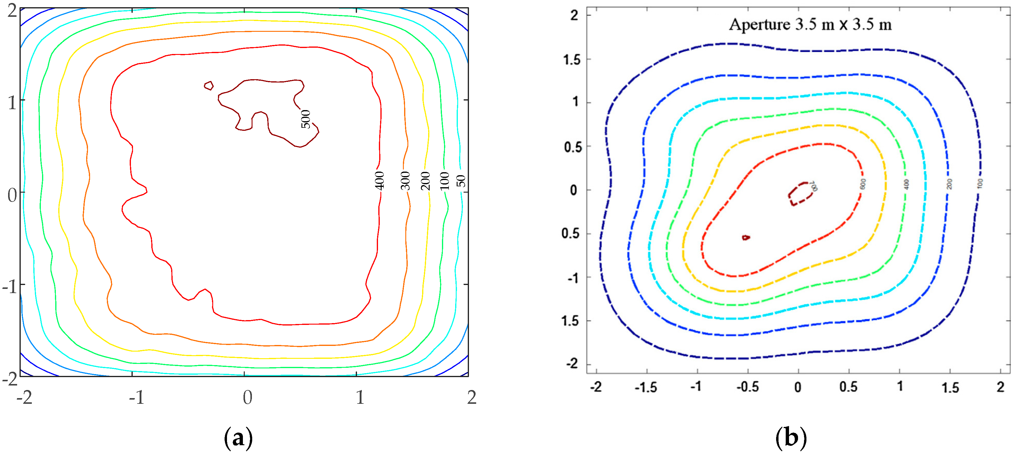
In order to more intuitively observe the comparative results, the unit in our paper was converted into the same unit of that in reference [12]. It could be seen that, after optimization, the peak solar flux density obtained in our paper was 500 suns, which was 200 suns lower than that in reference [12]. At the same time, the distribution area of solar flux in our paper seemed to be more extensive with the same incident energy. The radius of 400 suns was about 1.2 m in our paper and 1 m in reference [12]. In regard the spillage loss, the value after optimization in our paper was 8.67%, which was only increased by 0.84% (the value in reference [12] was 7.83%). This difference is fully acceptable. From the comparative result, it can be noted that the optimization strategy adopted in this paper can more effectively reduce the peak solar flux density on the receiver surface. Meanwhile, the solar flux distribution seems to be more uniform. Ultimately, it seems that the optimized dispatch proposed in this paper can meet the requirements for the safe operation of a central receiver.

A heliostat field plays a critical role in an entire solar thermal power tower plant and serves as its energy source. In this study, a “concentrating-receiver system” of 1 a MWe CSP Plant in Yanqing was selected as the research object to establish a spliced reflection model in the first place. Then, a grouping approach of heliostat fields was proposed according to the facts that heliostats in different positions have different contribution degrees and the incidence cosines of adjacent heliostats share resemblances. The selection principles of focal points are also designed based on spot sizes. Finally, an optimized dispatch and operation strategy have been confirmed for the heliostat field to realize an optimization goal of minimizing the standard deviation of solar flux distribution. It has been proven that the optimized dispatch strategy can be used to tremendously lower the peak values of solar flux densities on the receiver and to achieve uniform flux distribution. This is of great significance to extend the service life of a receiver and ensure that the receiver runs in a safe and stable state.

References

1. Desideri, U.; Campana, P.E. Analysis and comparison between a concentrating solar and a photovoltaic power plant. Appl. Energy 2014, 113, 422–433. [Google Scholar] [CrossRef]
2. Behar, O.; Khellaf, A.; Mohammedi, K. A review of studies on central receiver solar thermal power plants. Renew. Sustain. Energy Rev. 2013, 23, 12–39. [Google Scholar] [CrossRef]
3. Richardg.newell Daniel-Raimi-Gloria-Aldana. Global Energr Outlook 2019: The Next Genengeneration of Energy. Available online: https://www.rff.org/publications/reports/global-energy-outlook-2019/ (accessed on 1 July 2019).
4. Llamas, J.M.; Bullejos, D.; Ruiz de Adana, M. Optimization of 100 MWe Parabolic-Trough Solar-Thermal Power Plants under Regulated and Deregulated Electricity Market Conditions. Energies 2019, 12, 3973. [Google Scholar] [CrossRef]
5. Zhan, J.; Wang, Z. Solar Thermal Power Generation Technology in a New Generation of Energy System Positioning. Adv. Energy Power Eng. 2018, 6, 1–9. [Google Scholar] [CrossRef]
6. Dunnan, L.; Xiaodan, G.; Bowen, X. What causes growth of global greenhouse gas emissions? Evidence from 40 countries. Sci. Total Environ. 2019, 661, 750–766. [Google Scholar]
7. Du, E.; Zhang, N.; Hodge, B.-M.; Wang, Q.; Xia, Q. The Role of Concentrating Solar Power Towards High Renewable Energy Penetrated Power Systems. IEEE Trans. Power Syst. 2018, 33, 6630–6641. [Google Scholar] [CrossRef]
8. Besarati, S.M.; Yogi Goswami, D.; Stefanakos, E.K. Optimal heliostat aiming strategy for uniform distribution of heat flux on the receiver of a solar power tower plant. Energy Convers. Manag. 2014, 84, 234–243. [Google Scholar] [CrossRef]
9. Li, W.; Ma, J. Researches and simulation on heliostat concentrating strategy in solar power tower system. Renew. Energy Resour. 2016, 34, 475–480. [Google Scholar]
10. Yu, Q.; Wang, Z.; Xu, E. Analysis and improvement of solar flux distribution inside a cavity receiver based on multi-focal points of heliostat field. Appl. Energy 2014, 136, 417–430. [Google Scholar] [CrossRef]
11. Fernandez, N.; Street, A.; Montenon, A.; Maussion, P. A Scheduling Optimization Model for Sun Tracking of an Autonomous Heliostat. Available online: https://ieeexplore.ieee.org/stamp/stamp.jsp?tp=&arnumber=6652249 (accessed on 1 July 2019).
12. Salomé, A.; Chhel, F.; Flamant, G.; Ferrière, A.; Thiery, F. Control of the flux distribution on a solar tower receiver using an optimized aiming point strategy: Application to THEMIS solar tower. Sol. Energy 2013, 94, 352–366. [Google Scholar] [CrossRef]
13. Guo, T.; Liu, G.; Liu, D.; Guo, S. Research on Supreheated Evaluation Mode of Receiver on Solar Power Tower Plant and Dispatching Methods of heliostats Field. Acta Energ. Sol. Sin. 2014, 35, 166–170. [Google Scholar]
14. GarcÍa-MartÍn, F.J.; Berenguel, M.; Valverde, A.; Camacho, E.F. Heuristic knowledge-based heliostat field control for the optimization of the temperature distribution in a volumetric receiver. Sol. Energy 1999, 66, 355–369. [Google Scholar] [CrossRef]
15. Maffezzoni, C.; Parigi, F. Dynamic analysis and control of a solar power plant—II. Control system design and simulation. Sol. Energy 1982, 28, 117–128. [Google Scholar] [CrossRef]
16. Gallego, A.J.; Fele, F.; Camacho, E.F. On the optimization of irradiance distribution in solar tower plants with flat receivers. In Proceedings of the 2014 European Control Conference (ECC), Strasbourg, France, 24–27 June 2014. [Google Scholar]
17. Pitz-Paal, R.; Schwarzbozl, P.; Ulmer, S.; Belhomme, B. A New Fast Ray Tracing Tool for High-Precision Simulation of Heliostat Fields. J. Sol. Energy Eng. 2009, 131, 031002. [Google Scholar]
18. Xu, M. Study on Modeling and Control Strategy of Solar Thermal Power Condensing System. Ph.D. Thesis, Nan Jing Normal University, Nanjing, China, 2012. [Google Scholar]
19. Ding, T.; Hu, X. Application Research of Heliostats Field Scheduling with Intelligent Algorithm. Acta Energ. Sol. Sin. 2014, 35, 2139–2144. [Google Scholar]
20. Xu, E.; Yu, Q.; Wang, Z.; Yang, C. Modeling and simulation of 1 MW DAHAN solar thermal power tower plant. Renew. Energy 2010, 36, 848–857. [Google Scholar] [CrossRef]
21. Sun, F. Study on the Heliostat Tracking Correction System in a Solar Tower Power Plant. Ph.D. Thesis, The University of Chinese Academy of Sciences, Beijing, China, 2014. [Google Scholar]
22. Ballestrín, J.; Carra, M.E.; Enrique, R.; Monterreal, R.; Fernández-Reche, J.; Polo, J.; Casanova, M.; Barbero, F.J.; Marzo, A. Diagnosis of a Lambertian target in solar context. Measurement 2018, 119, 265–269. [Google Scholar] [CrossRef]
23. Liu, Y. Theoretical and Experimental Result of Focal Spot Flux Density Distribution of Solar Energy Concentrations. Ph.D. Thesis, HaRBin Institute of Technology, Harbin, China, 2008. [Google Scholar]
24. Zhou, Y. Research on Flux Distribution Simulation and Focus Strategy of TSP Plant. Master’s Thesis, ZheJiang University, Zhejiang, China, 2014. [Google Scholar]
25. Zhao, Q. Optimization on the Schedualing of the Heliostat Field in a Solar Tower Power Plant. Master’s Thesis, ZheJiang University, Zhejiang, China, 2017. [Google Scholar]
26. Koza, J.R. An Introduction to Genetic Algorithms; MIT Press: Boston, MA, USA, 1996. [Google Scholar]
27. Lei, Y.; Zhang, S.; Li, X.; Zhou, C.M. MALAB Genetic Algorithm Toolbox and Applications; XiDian University Press: Xian, China, 2014. [Google Scholar]
28. Mokshin, A.V.; Mokshin, V.V.; Sharnin, L.M. Adaptive Genetic Algorithms Used to Analyze Behavior of Complex System. Commun. Nonlinear Sci. Numer. Simul. 2018, 2019, 174–186. [Google Scholar] [CrossRef]
29. Ballestrín, J.; Casanova, M.; Monterreal, R.; Fernández-Reche, J.; Setien, E.; Rodríguez, J.; Galindo, J.; Barbero, F.J.; Batlles, F.J. Simplifying the measurement of high solar irradiance on receivers. Application to solar tower plants. Renew. Energy 2019, 138, 551–561. [Google Scholar] [CrossRef]
Figure 1. A perspective view of the heliostat field in the Yanqing concentrated solar power (CSP) plant.
Energies 12 04544 g001
Figure 2. A layout drawing of the heliostat field’s coordinates in the Yanqing CSP plant.
Energies 12 04544 g002
Figure 3. Working diagram of the beam characterization system (BCS).
Energies 12 04544 g003
Figure 4. Surface shape of heliostat in the Yanqing CSP plant.
Energies 12 04544 g004
Figure 5. A schematic diagram of the heliostat model.
Energies 12 04544 g005
Figure 6. Solar spot shape by the ideal and the spliced mirror surfaces. (a) Solar spot of the ideal surface. (b) Solar spot of the spliced surface.
Energies 12 04544 g006
Figure 7. Comparison result of simulation and experimental data for the solar flux distribution of the No. 5 focal point. (a) Solar flux distribution of the simulation result. (b) Solar flux distribution of the experimental result.
Energies 12 04544 g007
Figure 8. Comparison result of simulation and experimental data for the solar flux distribution of the No. 4 focal point. (a) Solar flux distribution of the simulation result. (b) Solar flux distribution of the experimental result.
Energies 12 04544 g008aEnergies 12 04544 g008b
Figure 9. Relation curves of solar spot energy percentage and radius. (a) Spot energy percentage of the No. 5 focal point. (b) Spot energy percentage of the No. 4 focal point.
Energies 12 04544 g009
Figure 10. A schematic diagram of heliostat concentrating and focal point selecting.
Energies 12 04544 g010
Figure 11. Incidence cosines of heliostats on different positions of the heliostat field.
Energies 12 04544 g011
Figure 12. A schematic diagram of heliostat field regionalization.
Energies 12 04544 g012
Figure 13. Flow chart of heliostat field optimization.
Energies 12 04544 g013
Figure 14. Distribution of focus points on a 4 × 4 m receiver surface.
Energies 12 04544 g014
Figure 15. Comparative results of solar flux distribution on receiver surface at 9:00 AM.(a) Flux distribution for simulation (plane graph). (b) Flux distribution for simulation (perspective view). (c) Flux distribution for experiment (plane graph). (d) Flux distribution for experiment (perspective view).
Energies 12 04544 g015
Figure 16. Comparative results of solar flux distribution on receiver surface at 12:00 AM. (a) Flux distribution for simulation (plane graph). (b) Flux distribution for simulation (perspective view). (c) Flux distribution for experiment (plane graph). (d) Flux distribution for experiment (perspective view).
Energies 12 04544 g016
Figure 17. Comparative results of solar flux distribution on receiver surface at 15:00 PM. (a) Flux distribution for simulation (plane graph). (b) Flux distribution for simulation (perspective view). (c) Flux distribution for experiment (plane graph). (d) Flux distribution for experiment (perspective view).
Energies 12 04544 g017
Figure 18. Flux distribution on the receiver surface after heliostat field regionalization. (a1a3) Flux distribution (plane graph) based on multi-point Focusing. (b1–b3) Flux distribution (perspective view) based on multi-point Focusing. (c1–c3) Flux distribution (plane graph) based on central point focusing. (d1–d3) Flux distribution (perspective view) based on central point focusing.
Energies 12 04544 g018aEnergies 12 04544 g018b
Figure 19. Flux distribution on the receiver surface central profiles. (a) Flux distribution on horizontal profiles. (b) Flux distribution on vertical profiles.
Energies 12 04544 g019aEnergies 12 04544 g019b
Figure 20. Comparative results of solar flux distribution on the receiver surface of the Themis plant. (a) The result with the GA. (b) The result with TABU.
Energies 12 04544 g020