Optimal Design of a Diesel-PV-Wind-Battery-Hydro Pumped POWER system with the Integration of ELECTRIC vehicles in a Colombian Community

Abstract

This article proposes a novel design methodology for hybrid isolated microgrids, integrating electric vehicles (EV) as additional loads and also as additional storage systems in the microgrid design stage. The proposed method highlights the application of electric vehicles in rural environments. Two types of electric vehicles were considered: (1) EV that only operate in charging mode; and (2) EV that can interchange power with the microgrid (V2G). For both EV types, a dispatch strategy was developed to optimize the use of the system resources during the charging process. As an application example of the proposed design methodology, a hybrid microgrid was designed for the rural Colombian village of Unguía. The results show the advantages of the inclusion of EV as ancillary services providers for the system and also as public transportation agents.

1. Introduction

Nowadays, access to electricity is one of the most critical aspects when assessing the degree of welfare and development of people [1]. For the particular case of Colombia, the population with a regular supply of electricity provided by the primary grid system is located around the big urban centers corresponding to 48% of the territory; this also means that more than half of the country belongs to the so-called non-interconnected zones (NIZ) [2]. Although the Colombian government has a sponsored program for fuel distribution for diesel plant operation in the NIZ, transportation problems elevate the costs and decrease the effectiveness of these solutions, and the environmental concerns also have to be accounted for [2]. In this context, many alternatives have been proposed for decreasing the economic and environmental consequences of fuel-based energy sources in the country [3]. These alternatives include the use of hybrid microgrid systems involving renewable energy sources and the existent diesel plants, which emerge as a promising initiative for the increment of the electricity access in Colombian non-interconnected zones [2].

As defined in [4], microgrids can be considered as systems composed of loads and at least one element of small-scale distributed generation (DG) or storage with the ability to operate disconnected from the primary power grid. As the interest in microgrids grows, aspects such as the optimal configuration of distributed generation or the adequate management of the energy sources arise as research questions. Several works have addressed those issues [5,6], with microgrid design approaches classified as deterministic or stochastic according to the modeling of input variables such as expected demand and weather forecasting [7]. Microgrid design also involves the determination of the combination of elements making possible the fulfillment of the power balance in the microgrid according to some predefined criteria. The search for the optimal microgrid configuration involves mainly enumeration techniques (used for the popular design software HOMER^®), iterative approaches, and artificial intelligence methods [8]. However, each technique has disadvantages such as the high computational times, the lack of multi-objective cost functions, or the convergence towards local minimum because of the non-convexity of the formulated problems [9]. Despite considerable interest, the optimal microgrid design problem remains an open research area.

In this context, the microgrid application for electricity generation in rural zones faces additional challenges. For the population of the Colombian NIZ, the joint action of storage and generation elements must be able to supply the demanded energy. These storage elements can be battery banks, hydro-pumped systems, or even electric vehicles (EV). The consideration of EV operation in power systems constitutes a challenge that has been widely discussed, mainly due to the worldwide efforts for reducing fossil-fuel dependence and greenhouse gas emissions [10,11]. According to Wappelhorst et al. [12], the use of EV should be considered a priority to reduce energy consumption around the world.

In the specialized literature, the authors of [13,14] presented comprehensive summaries of the different strategies and research issues on integration of EVs in power grids. Generally speaking, vehicle-to-grid (V2G) connection mode enables the electric vehicle to participate as both a distributed source and a controllable load for the grid [14]. Several works have explored the operation of EV in microgrids; some of the specific issues and technical challenges related to EV role in microgrids are presented in [15,16,17]. In particular, the expected operating costs of a microgrid dealing with EV and responsive loads with the participation of distributed renewable energy sources were calculated in [10], including carbon emissions. The mix of different generation sources decreases both the overall microgrid costs and the uncertainties in solar and wind sources. Furthermore, the work presented in [18] considers the inclusion of EVs in a microgrid composed of diesel generators, fuel cells, microturbines, and photovoltaic panels. The power delivered by diesel generators and the power exchanged between EVs and power grid are calculated through an optimization process that minimizes the operation and emissions costs.

Despite the recent interest, there are not many works studying the application of EVs in rural scenarios and their inclusion from the microgrid design stage. Many of the reasons for this lack of research seem to involve topics such as the high purchase price of the EVs and the lack of the infrastructure (charging stations, replacement parts, and qualified technical operators) to support the integration [19]. However, the potential for development in non-urban scenarios is real. According to Wappelhorst et al. [12], some of the benefits provided by electric vehicles in urban areas (such as improving public transport in the community, reducing pollutants, etc.) are also feasible and replicable for rural environments. In this sense, this work intends to explore the inclusion of EV in an isolated microgrid for a rural environment. In fact, from the results of Falcão et al. [20] indicating that EVs as storage systems reduce the microgrid operational costs, this work extends the inclusion of EVs into the design stage of the microgrid to determine the impacts in the microgrid sizing. The proposed design methodology for hybrid isolated microgrids uses an iterative optimization method for solving the unit commitment problem in the microgrid, including the EV, as in [10,18]. We extend the latter works by including the rated power of the microgrid elements as decision variables in our optimization. Hence, both the optimal planning and optimal dispatch problems can be addressed simultaneously.

The proposed design methodology was applied in a Colombian rural community, considering a microgrid composed of a diesel plant, solar photovoltaic (PV) panels, wind turbines, batteries, a hydro-pumped system, and EVs. The role of EVs in the rural community is envisioned as public service vehicles, performing tasks such as the transportation of the staff of a hospital or a public institution from a central station to the attention point. Two operational modes for EVs are studied: EVs that only constitute additional loads for the microgrid, and EVs that provide ancillary services.

This article is organized as follows. Section 2 describes the modeling of the generation elements composing the hybrid microgrid. Section 3 presents the formulation and solution of the optimization problem for microgrid design. The study case for the isolated microgrid design is described in Section 4. Finally, the analysis and discussion of the results are shown in Section 5.

2. Modeling of Microgrid Elements

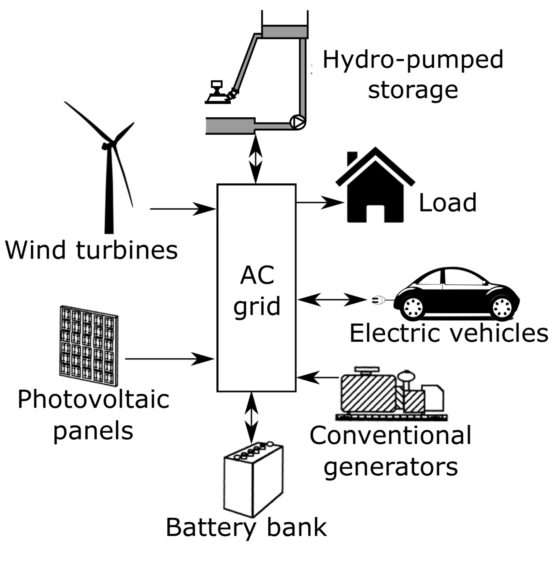
The proposed microgrid is composed of a diesel generator, a battery bank, a hydro-pumped storage system, solar panels, wind turbines, and EVs. A schematic figure of a hybrid microgrid such as the one considered is illustrated in Figure 1.

In this section, only the models for EV are discussed in detail. The models for the remaining microgrid elements come from the current literature. The models for wind turbines, batteries, and diesel generators are from the work of Maleki and Askarzadeh [21], the photovoltaic panels use the model described in [22], and the hydro-pumped storage can be found in [23].

2.1. Modeling of Electric Vehicles

As described above, the microgrid to be designed is proposed for an off-grid system, intended for supplying electricity for a rurally isolated area. This fact defines the pattern consumption of electric vehicles and the strategy for their integration with the power grid. The assumption is that electric vehicles will provide a transportation service for the community public institutions functionaries, as this eliminates the dependence of fossil fuels that must be transported to the remote area and decreases the carbon emissions [12]. For rural zones, small-sized EVs are considered as the population incomes are usually low, the traveling distances are short, and motorcycles do not cover all the transportation needs of the people [24].

In this context, one vehicle is assigned to each relevant institution in the community. As suggested in [25], central community institutions usually include the following: offices of local, state, and government agencies, religious institutions, cultural institutions, community centers, hospitals and public health service, educative centers, and public sports facilities. In addition, as the electric vehicles considered are of low capacity, it is feasible to assume a low rate of charge for them (less than 2 kW/h). Therefore, the existence of a particular charging station is not required, and the vehicles could be charged with a typical home circuit of 220 V. From their role in the electric microgrid, two types of EVs are considered: Type 1, acting as dynamic loads, and Type 2 with active participation in the grid as additional storage elements.

2.2. Type 1 Electric Vehicles

These vehicles perform as additional loads in the grid power balance. The microgrid system will provide the required energy to this type of EV to achieve the full charge in the charging schedule. The energy management system will dynamically assign the charging power according to resource availability. Type 1 EVs are intended for the use of institutions providing priority care services in the community, such as hospitals and police stations. The charging schedule will be scheduled according to the working hours of each institution.

2.3. Type 2 Electric Vehicles

Type 2 EVs participate as additional storage systems during the parking hours. As a design condition, a minimum level of charge must be guaranteed at the beginning of the daily working hours in order to execute the programmed trips. These vehicles will be assigned to the offices of local institutions such as the mayor’s office and deputies since these entities do not need to deal with unforeseen situations as frequently as the hospital and the police institutions. Therefore, recognizing the stochastic nature of the driving pattern for the Type 2 EVs, the daily consumption of these vehicles will be calculated using a probability density function.

The daily energy consumption of Type 2 EVs determines the surplus energy in their batteries, which will be delivered to the network again if the system requires it. According to Wu et al. [11], the daily travel distances of electric vehicles used by office staff behave as a Log-normal stochastic process, based on the travel distances recorded by the National Household Travel Survey in [26]. Thus, a Log-normal probability density distribution $f\left(d\right)$ is used to approximate the daily driving distances:

$$f\left(d\right)=\frac{1}{d\sigma \sqrt{2\pi }}{e}^{\left(-\frac{ln\left(d\right)-\mu }{2{\sigma }^2}\right)},$$

(1)

where d is the distance traveled by a vehicle during a trip (km), $\mu$ is the average traveled distance at the design period, and $\sigma$ is the standard deviation of the traveled distances. The parameters of the Log-normal function are estimated from previously known travel distances of the designated institution’s schedules or assuming the execution of a given number of travels to the neighboring places or towns near to the operating region.

With the Lognormal distribution function already characterized, daily traveling distances $d\in R^p$ (being p the number of days in the design period) are randomly generated for the whole design period, and the same daily routes are assumed for all the Type 2 EVs. Then, these distances are multiplied by two to represent the round trip distance. In addition, several trips can be performed during the same day; hence, the vector ${\mathit{n}}_{\mathit{v}}\in R^p$ of the number of trips per day is randomly generated using a binomial probability distribution. Thus, the daily energy consumption ${\mathit{G}}_{\mathit{v}\mathit{2}}$ of each Type 2 EV is:

$${\mathit{G}}_{\mathit{v}\mathit{2}}=2G_v\mathit{d}·{\mathit{n}}_{\mathit{v}}.$$

(2)

In Equation (2), $G_v$ is the energetic consumption produced by driving an EV (kWh km⁻¹). The equation of battery energy for a Type 2 EV ($E_{v2}$) is analogous to the equation of the energy in the battery bank in [11]. However, for electric vehicles, the efficiency of charging and discharging of the battery is assumed to be 100%. This gives the following equation:

$$E_{v2}(t+1)=E_{v2}\left(t\right)(1-{\gamma }_v)+\left(P_{v2,c}\left(t\right)-P_{v2,d}\left(t\right)\right),\forall t\in 1,2,\dots ,N;$$

(3)

where N is the number of time steps in the design period, ${\gamma }_v$ is the self-discharge coefficient of the battery, $P_{v2,c}\left(t\right)$ is the charging power, and $P_{v2,d}\left(t\right)$ is the discharging power of the batteries at the time step t. Besides, the initial charging of the batteries of electric vehicles $E_{v2}\left(0\right)$ is assumed as the minimum energy level.

3. Formulation of the Optimization Problem

The variables calculated by the optimization are classified as size variables and dispatch variables. The dispatch variables are the power delivered by the Diesel generators at each time step ${\mathit{P}}_{\mathit{G}}\in R^N$; the charging and discharging power of the battery bank at each time step denoted by ${\mathit{P}}_{\mathit{b},\mathit{c}}\in R^N$ and ${\mathit{P}}_{\mathit{b},\mathit{d}}\in R^N$; the power consumption of the water pump and the power generated by the hydraulic turbine of the hydro-pumped storage system at each time step, denoted by ${\mathit{P}}_{\mathit{wp},\mathit{c}}\in R^N$ and ${\mathit{P}}_{\mathit{wp},\mathit{d}}\in R^N$; the charging power of Type 1 EVs at each time step ${\mathit{P}}_{\mathit{v}\mathbf{1},\mathit{c}}\in R^N$; the charging and discharging power of Type 2 EVs at each time step, ${\mathit{P}}_{\mathit{v}\mathbf{2},\mathit{c}}\in R^N$ and ${\mathit{P}}_{\mathit{v}\mathbf{2},\mathit{d}}\in R^N$ (only the charging power is considered as a decision variable for Type 1 EV); and the unsupplied demand at time step ${\mathit{P}}_{\mathit{us}}\in R^N$. The designer defines the number of EVs of each type as input data.

Size variables are the number of photovoltaic panels $N_{pv}$, the number of wind turbines $N_{wt}$, the number of batteries in the battery bank $N_b$, the water storage tank volume V, the rated power of the pump $P_{wp,c}^M=max\left({\mathit{P}}_{\mathit{wp},\mathit{c}}\right)$ and the rated power of the hydraulic turbine $P_{wp,d}^M=max\left({\mathit{P}}_{\mathit{wp},\mathit{d}}\right)$. Vector x lists the decision variables as:

$$x^T=\left[\begin{array}{ccccccccccccc}{N}_{pv}& N_{wt}& N_b& V& {\mathit{P}}_{\mathit{G}}^T& {\mathit{P}}_{\mathit{b},\mathit{c}}^T& {\mathit{P}}_{\mathit{b},\mathit{d}}^T& {\mathit{P}}_{\mathit{wp},\mathit{c}}^T& {\mathit{P}}_{\mathit{wp},\mathit{d}}^T& {\mathit{P}}_{\mathit{v}\mathbf{1},\mathit{c}}^T& {\mathit{P}}_{\mathit{v}\mathbf{2},\mathit{c}}^T& {\mathit{P}}_{\mathit{v}\mathbf{2},\mathit{d}}^T& {\mathit{P}}_{\mathit{us}}^T\end{array}\right]$$

(4)

Under the assumption of diesel generation already existing in the rural community of microgrid operation, the number of diesel generation units is not included in the decision variables. Hence, the initial diesel generation investments are also not considered.

3.1. Objective Function

A multi-objective weighted function was employed to calculate the design with the lowest possible cost. Two objectives compose this function: the total yearly system cost ($C_T$) and the total yearly system emissions ($E_T$), with the latter weighted by the factor $w_E$. The objective function f is presented in Equation (5).

$$f\left(x\right)=C_T\left(x\right)+w_E{E}_T\left(x\right)$$

(5)

The designer must define the value of the emissions weight coefficient concerning the cost associated with the $C{O}_2$ emissions. Here, this cost is extracted from the $C{O}_2$ Negotiation European System [27] at the microgrid location.

3.1.1. Total System Cost

For the time period accounted for in the design, the total system cost is calculated as in [28]:

$$C_T\left(x\right)=C_{in}\left(x\right)+C_{mt}\left(x\right)+C_G\left(x\right),$$

(6)

where $C_{in}$ is the annualized initial investment cost, $i_n$ is the interest rate, n is the project lifespan, $C_{mt}$ is the maintenance cost, and $C_G$ is the cost associated with diesel generation. The annualized initial investment cost ($C_{in}$) is calculated as indicated in Equation (7):

$$C_{in}\left(x\right)=CRF\left(\sum _{j=pv,wt,b}{N}_j{C}_{in}^j+\sum _{l=c,d}{P}_{wp,l}^M{C}_{in}^{wp,l}+V{C}_{in}^v+\sum _{m=v1,v2}{N}_m{C}_{in}^m+C_{Tr}\left(x\right)+C_{rp}\left(x\right)\right).$$

(7)

In Equation (7), $N_j$ is the number of units of the type j element. Sub-index j takes the following values: $j=wt$ for wind turbines, $j=pv$ for photovoltaic panels, and $j=b$ for batteries of the battery bank. In addition, sub-index $l=c$ indicates a charging state of the storage system and $l=d$ indicates a discharging state. The term $C_{in}^j$ is the initial investment cost for the type j element, and $CRF$ is the capital recovery factor.

In addition, investment cost includes the replacement cost $C_{rp}$ for elements with a lifespan lower than the project lifespan (batteries and converters of both photovoltaic panels and batteries) and the cost $C_{Tr}$ of the occupied land by the microgrid elements. This latter cost is associated with the use of the land, and it is calculated by the following expression:

$$C_{Tr}\left(x\right)=C_g\left(\sum _{j=pv,wt,b}{N}_j{A}_j\right),$$

(8)

where $C_g$ is the land price index and $A_j$ is the area occupied by the generation element of type j. The maintenance cost ($C_{m}t$) is calculated as:

$$C_{mt}\left(x\right)=\sum _{j=pv,wt,b}{N}_j{C}_{mt}^j+\sum _{l=c,d}{P}_{wp,l}^M{C}_{mt}^{wp,l}+N_G{C}_{mt}^G,$$

(9)

where $C_{mt}^k$ is the maintenance cost for element k. The cost associated with the fuel for diesel generation is given by Equation (10):

$$C_G\left(x\right)=\sum _{t=1}^N\left[{\mathit{G}}_{\mathit{df}}\left(t\right){\mathit{C}}_{\mathit{df}}\left(t\right)+C_l{\mathit{G}}_{\mathit{l}}\left(t\right)\right]\frac{T}{N}.$$

(10)

In Equation (10), T is the number of time steps in one year, ${\mathit{G}}_{\mathit{df}}\in R^N$ is the consumption of the diesel fuel at each time step, and ${\mathit{C}}_{\mathit{df}}\in R^N$ is the fuel cost at each time step. $C_l$ denotes the cost of the lubricant (which is assumed as constant) and ${\mathit{G}}_{\mathit{l}}\in R^N$ is the diesel generator lubricant expense, which is related to fuel consumption by the following expression:

$${\mathit{G}}_{\mathit{l}}=0.001226·{\mathit{P}}_{\mathit{G}}.$$

(11)

In Equation (11), $P_G$ denotes the power delivered by the diesel generator in $\left[\mathrm{kW}\right]$. Equations (10) and (11) were both taken from [29].

3.1.2. Total Carbon Emissions of the System

The design problem assumes the microgrid generating $C{O}_2$ emissions at both the construction and operation stages only. The emissions during the operation stage are exclusively due to diesel fuel combustion.

$$E_T\left(x\right)=\sum _{j=pv,wt}{N}_j{P}_j^M{E}_c^j+\sum _{h=b,wp}{N}_h{E}_h^M{E}_c^j+\left[\sum _{t=1}^N{E}_{op}^G{G}_{df}\left(t\right)\right]\frac{T}{N}.$$

(12)

Equation (12) shows the total calculation of $C{O}_2$ emissions, where $P_j^M$ is the rated power of the type j element, $E_c^j$ represents the $C{O}_2$ emissions produced by construction of the type j element, $E_h^M$ is the maximum energy capacity of the type h storage system, and $E_{op}^G$ denotes the $C{O}_2$ emissions produced by diesel fuel combustion.

3.2. Constraints

The optimization problem has constraints that determine the requirements for its solution. Constraints come from operational conditions of the elements and aspects such as the reliability in the energy supply. The following subsections describe the mathematical expressions for the constraints considered in the microgrid design.

3.2.1. Design Constraints

These are the constraints related to the nature of the design problem and operational limits of the generation elements. First, all decision variables must be positive values, and the variables related to the number of elements must be integer numbers.

$$N_j,V\ge 0;N_j\in \mathbb{N}j=wt,pv,b$$

(13)

$${\mathit{P}}_{\mathit{G}},{\mathit{P}}_{\mathit{h},\mathit{c}},{\mathit{P}}_{\mathit{h},\mathit{d}},{\mathit{P}}_{\mathit{us}}\ge \mathbf{0}h=b,wp,v1,v2.$$

(14)

The energy stored in the battery bank and EV batteries must remain between the allowable maximum and minimum limits:

$$N_h·E_h^m\le {\mathit{E}}_{\mathit{h}}\left(t\right)\le N_h·E_h^{M}h=b,v2,\forall t=1,\dots ,N.$$

(15)

In Equation (15), ${\mathit{E}}_{\mathit{h}}\left(t\right)$ is the energy stored in the type h storage system at the time step t (with $h=b$ for battery bank and $h=v2$ for batteries of Type 2 EV). $E_h^m$ and $E_h^M$ are the minimum and maximum energy capacity of the type h storage system, respectively.

The energy stored in the the water tank ${\mathit{E}}_{\mathit{wp}}$ is limited by the tank capacity:

$$E_{wp}^m\le {\mathit{E}}_{\mathit{wp}}\left(t\right)\le V\forall t=1,\dots ,N.$$

(16)

The dispatch variables must be kept between defined maximum and minimum values:

$$0\le {\mathit{P}}_{\mathit{G}}\left(t\right)\le P_G^M\forall t=1,\dots ,N$$

(17)

$$0\le {\mathit{P}}_{\mathit{h},\mathit{c}}\left(t\right)\le P_{h,c}^M\forall t=1,\dots ,Nh=b,wp,v1,v2$$

(18)

$$0\le {\mathit{P}}_{\mathit{h},\mathit{d}}\left(t\right)\le P_{h,d}^M\forall t=1,\dots ,Nh=b,wp,v1,v2$$

(19)

$$0\le {\mathit{P}}_{\mathit{us}}\left(t\right)\le {\mathit{P}}_{\mathit{l}}\left(t\right)\forall t=1,\dots ,N$$

(20)

In Equations (17)–(20), $P_G^M$ is the total rated power of diesel generators and $P_{h,c}^M$ and $P_{h,d}^M$ are the maximum charging and discharging power of the type h storage system, respectively. The variable ${\mathit{P}}_{\mathit{l}}\in R^N$ denotes the load demanded in the microgrid at each step time.

3.2.2. Reliability Constraints

The reliability constraint is established in terms of the probability ($p_{ns}$) of loss of power supply. This probability is defined as the ratio of the total unsupplied demand to the total demand, over a chosen design period, as Equation (21) indicates.

$$p_{ns}=\sum _{t=1}^N{P}_{us}\left(t\right)/\sum _{t=1}^N{P}_l\left(t\right)\le R_L.$$

(21)

The designer must define the value of the system reliability level denoted by $R_L$. This variable is the lower bound for the probability of loss of power supply. Thus, $R_L$ indicates the minimum demand that the system will be able to supply. A complete expression for the loss of power supply may involve the representation of factors such as weather forecasts, demand and generation prediction, reliability indexes and equipment failure rates, similar to those performed in long-term planning studies [30].

3.2.3. Constraints for Electric Vehicles

Type 1 EV The operating period for the institution with assigned Type 1 EVs is between hours $h_{1i}$ to $h_{1f}$, and the non-working hours are between the interval $[h{{}^{\prime }}_{1i}$ and $h{{}^{\prime }}_{1f}]$. For a full charge, the energy injected to a Type 1 EV at the non-working period must be equal to or higher than the maximum allowed energy $E_{v1}^M$. This condition is set in Equation (22), where $E_{v1}^M$ is the maximum capacity of batteries of Type 1 EVs, and $h{{}^{\prime }}_{1i}$ and $h{{}^{\prime }}_{1f}$ denote the initial and final non-working hours for type1 EV, respectively.

$$\sum _{k=h{{}^{\prime }}_{1i}}^{h{{}^{\prime }}_{1f}}{P}_{v1,c}\left(k\right)\ge R_L{N}_{v1}{E}_{v1}^M.$$

(22)

In addition, the charging power must be zero during the working period, because the vehicles are in operation at that moment. This condition is set in Equation (23).

$$P_{v1,c}\left(k\right)\le 0\forall k\in \nu =\{h_{1i},\dots ,h_{1f}\}.$$

(23)

Type 2 EV The operating period for institutions with assigned Type 2 EVs is between hours $h_{2i}$ to $h_{2f}$, and the non-working hours are between the interval $[h{{}^{\prime }}_{2i}$ and $h{{}^{\prime }}_{2f}]$. The available power to discharge in a Type 2 EV $P_{v2,d}$ must equal to or greater than the daily driving average power consumption at the working hours. This average power consumption is obtained by dividing the total daily energy by the number of working hours, as indicated in Equation (24). The charge and discharge process of Type 2 EV batteries must comply with Equations (24) and (25).

$$P_{v2,d}\left(k\right)\ge R_L\left(N_{v2}\frac{G_{v2}}{h_{2f}-h_{2i}}\right)\forall k\in \nu =\{h_{2i},\dots ,h_{2f}\}.$$

(24)

The charging power of Type 2 EVs at working hours must be zero every day. This condition is expressed as follows:

$$P_{v2,c}\left(k\right)\le 0\forall k\in \nu =\{h_{2i},\dots ,h_{2f}\}$$

(25)

In addition, system power balance must condition the exchanged power with the grid by Type 2 EVs at the non-working hours from $h{{}^{\prime }}_{2i}$ to $h{{}^{\prime }}_{2f}$. This constraint is indicated in Equation (26), where $P{{}^{\prime }}_{v2,d}\left(k\right)$ is the power discharged by Type 2 EV to the grid at the non-working period.

$$P_l\left(t\right)\le \sum _{j=G,wt,pv}{N}_j{P}_j\left(t\right)-\sum _{h=b,wp}\left[P_{h,c}\left(t\right)+P_{h,d}\left(t\right)\right]+P{{}^{\prime }}_{v2,d}\left(t\right)-P_{v1,c}\left(t\right)+P_{us}\left(t\right).$$

(26)

3.2.4. Constraints for Diesel Fuel Availability

The last constraint deals with the unavailability of power from diesel generators due to factors such as fuel exhaustion, loss of line connectivity, or equipment failure [5]. For a broad representation of these situations, an average daily energy value of $G_G^M$ is set as the upper bound for the daily energy supplied by the diesel. Equation (27) describes daily energy delivered by diesel generators, where $h_i$ and $h_f$ are the initial and final hour for the days covered by the design period, respectively.

$$\sum _{t=h_i}^{h_f}{P}_G\left(t\right)\le G_G^M,$$

(27)

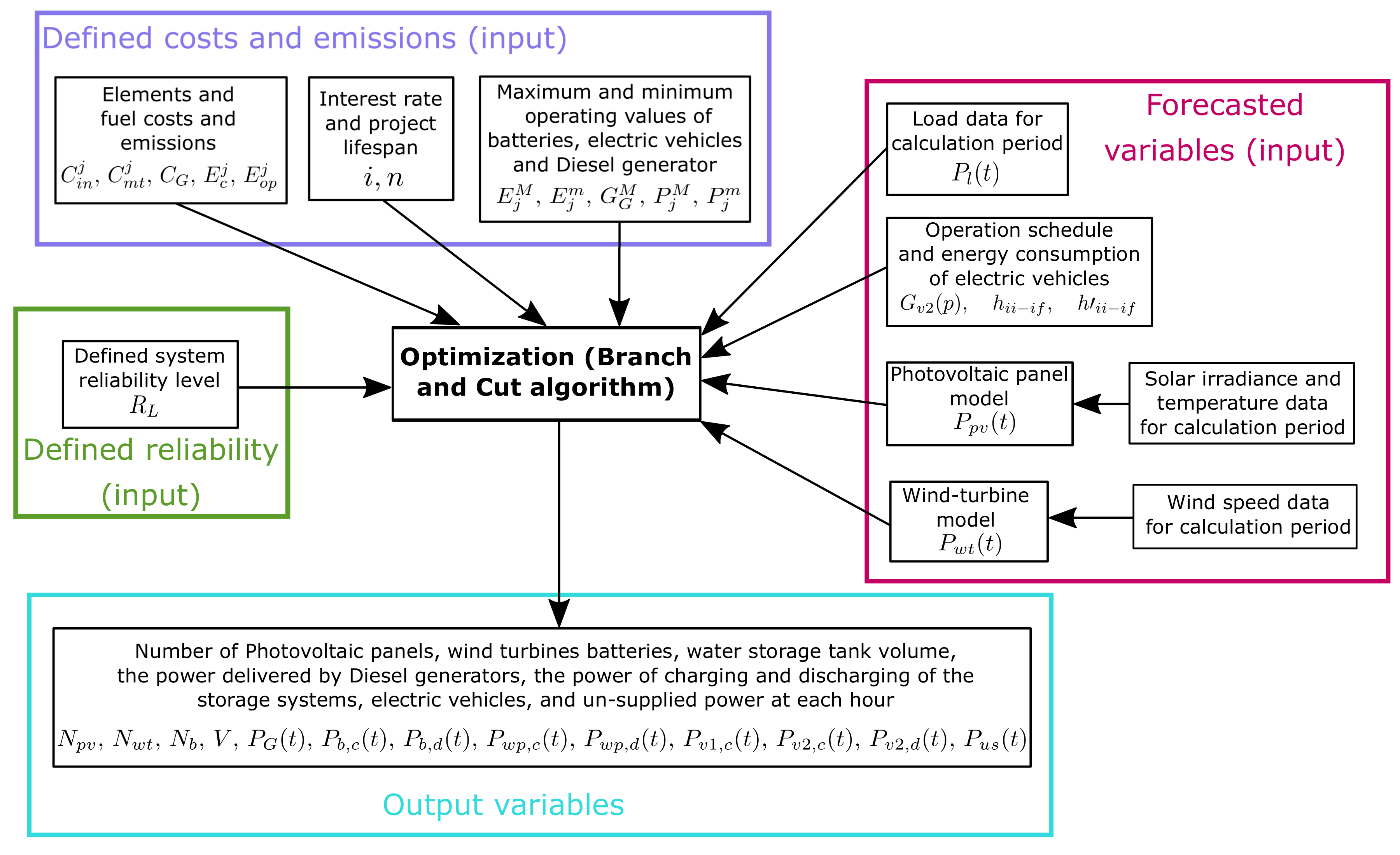
3.3. Solution Method

The cost function of the optimization problem in Section 3 has both linear and convex characteristics. These features come from the maximum point-to-point function $max\left(·\right)$ of a positive constant, as indicated in Equations (7), (9) and (12). Additionally, this problem has a mixed-integer nature, as integer numbers represent the amount of photovoltaic panels, wind turbines, batteries, and the volume of the water storage tank. In addition, variables for the power dispatch of each element are real-valued. Under these conditions, the branch and cut method was used to solve the resulting mixed-integer problem. Optimization was performed with software CVX in Matlab^® using Gurobi^® solver [31]. Figure 2 provides a graphic representation of the proposed solution method, summarizing all the involved variables.

4. Description of the Case of Study

The Colombian rural village of Unguía was selected to illustrate the application of the proposed microgrid design methodology. Unguía is a community located in the north of the Chocó department, at 478 km by waterway from Quibdó, the state capital. This rural community has an estimated population of 15,200 inhabitants [32], with around 31% of them in the urban area. The urban area has about 900 households, of which the 78% have access to electric service provided by two 475 kVA diesel generators. Unguía has public entities such as the Mayor’s Office; the Agrarian Bank; the Department for Social Prosperity; the secretaries of government, finance, and agriculture; a police station; and a hospital. In addition, there is an active presence of private actors, such as associations with legal status.

This community was selected based on the study by Gómez [33], highlighting Unguía as a good option for the implementation of solar and wind generation alternatives in Colombia. Weather variables and the demanded load were taken from 2015 data to perform the microgrid design. Information about demanded load was provided by Instituto de Planificación y Promoción de Soluciones Energéticas para las Zonas No Interconectadas [34]. However, these data series have periods when the demanded load was 0 kW. During these periods, the zero demand was replaced by the average weekly consumption obtained for days with total supply. The design scenario involves five small-sized EVs (Renault Twizy model), distributed as follows: the hospital and the police employ two Type 1 EVs, and the mayoralty, the court and the Secretary of Government use the remaining three vehicles as Type 2 EVs.

The Lognormal distribution parameters $\mu$ and $\sigma$ for Type 2 EVs were calculated by matching the data of travel distances with this distribution. The travel distance data were calculated as the average distances between the mayoralty, the court, the secretariat of government, and the rural villages that can be reached by road. In this way, the obtained parameter values were $\mu =$1.44416 y $\sigma =$0.630016. Furthermore, the energy storage limitations in EV batteries only allow for up to two trips per day, according to the distance to the furthest population. Hence, the number of trips per day was randomly generated using a binomial probability distribution with parameters $N=2$ and $p=0.5$.

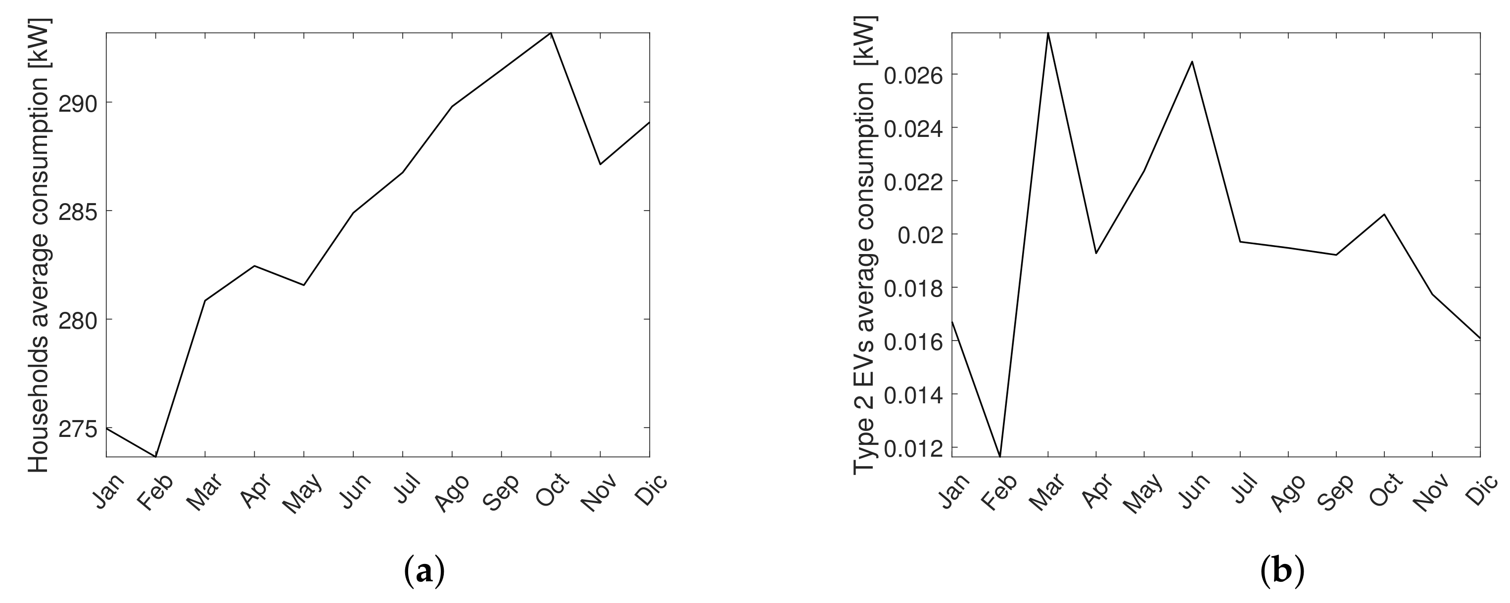
The operating period for the Type 1 EV was established from Monday to Sunday between 7:00 and 19:00. Besides, Type 2 vehicles would be operating from Monday to Friday between 8:00 and 18:00, in concordance with the schedule of public service entities at Unguía [32]. Figure 3a shows the monthly average of demanded load and Figure 3 shows the average power consumption by Type 2 EV. The total energy consumption of both elements was obtained by multiplying the average values by the number of hours in the month.

According to Figure 3b, power consumption of Type 2 EVs is much lower than the demanded power by household users (0.0044% of the latter). This behavior is expected, as 909 homes have a more significant power consumption (Figure 3a than only three small-sized electric vehicles, even for a rural community.

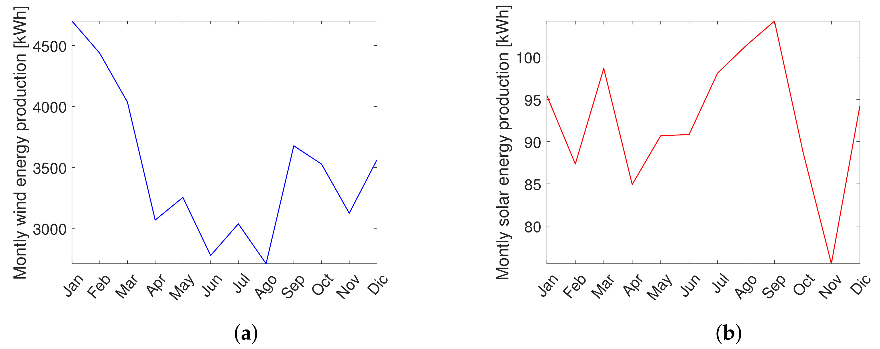
4.1. Meteorological Variables

A deterministic approach was used for weather forecasting, assuming the same behavior of previous years. Data time-series recorded from Unguía weather variables in 2016 approximated the weather conditions for the design period. These wind speed and temperature data were provided by IDEAM, a state entity in charge of environmental studies [35]. The solar irradiance incident on the photovoltaic panels at Unguía was obtained from the NASA database [36] through the software HOMER^® [37] for 2016. The hourly horizontal surface solar irradiance data series were calculated synthetically from the monthly average irradiance, through the application of the Graham algorithm. Calculations assumed the same tilt (5.99${}^{\circ }$) and azimuth (180${}^{\circ }$) angles for all photovoltaic modules. 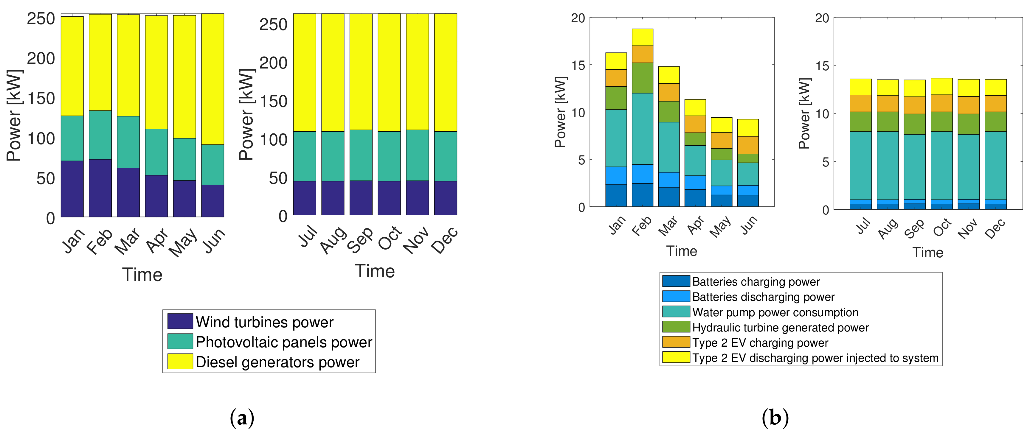Figure 4a,b illustrates the monthly energy production reached with one wind turbine and one photovoltaic panel at Unguía.

4.2. Parameters for Total Cost Calculation

The parameters assumed for calculation of total system cost were: time steps of 1 h, an annual interest rate $i_n$ of 5%, a project lifespan n of 20 years, and a weight coefficient of emissions $w_E$ of $8.49\mathrm{USD}/{\mathrm{t}}^{-1}\mathrm{CO}2$. This latter value corresponds to the annual average emissions cost for the European Union, set by SENDECO₂ for 2015 [27]. The complete list of the parameters for microgrid elements is presented in

Table A1. Technical characteristics of microgrid elements [41,43,44,45,46,47].

Nomenclature	Variable Description	Value
General microgrid
n	Lifespan	20 [years]
i	Interest rate	5%
$R_L$	Reliability level	0.2
$w_E$	Emissions cost	$\$0.01$$\left[\mathrm{USD}/\mathrm{k}{\mathrm{g}}^{-1}\mathrm{CO}2\right]$
$C_g$	Land price	$\$0.05$$\left[\mathrm{USD}{\mathrm{m}}^{-2}\right]$
Photovoltaic panel
$A_{pv}$	Occupied area	1.675 × 1.330 $\left[{\mathrm{m}}^2\right]$
$C_{in}^{pv}$	Investment cost	2216.4 [$\mathrm{USD}$]
$C_{mt}^{pv}$	Maintenance cost	2% of the investment cost
$E_c^{pv}$	$C{O}_2$ emissions in construction	1392 $\left[\mathrm{k}\mathrm{g}\mathrm{CO}2\mathrm{k}{\mathrm{W}}^{-1}\right]$
Wind turbine
$A_{wt}$	Occupied area	15,625 $\left[{\mathrm{m}}^2\right]$
$C_{in}^{wt}$	Investment cost	11,868 $\left[\mathrm{USD}\right]$
$C_{mt}^{wt}$	Maintenance cost	2% of investment cost
$E_c^{wt}$	$C{O}_2$ emissions in construction	675 $\left[\mathrm{k}\mathrm{g}\mathrm{CO}2\mathrm{k}{\mathrm{W}}^{-1}\right]$
Battery
$E_b^M$	Rated capacity	14.4 [kWh]
$A_b$	Occupied area	0.53 $\left[{\mathrm{m}}^2\right]$
$E_b^m$	Maximum discharge level	2.9 [kWh]
$P_{bc}^M$, $P_{bd}^M$	Maximum charge/discharge power	8 $\left[\mathrm{k}\mathrm{W}\right]$
$C_{in}^b$	Investment cost	3810 $\left[\mathrm{USD}\right]$
$C_{mt}^b$	Maintenance cost	2% of investment cost
$E_c^b$	$C{O}_2$ emissions in construction	59 $\left[\mathrm{k}\mathrm{g}\mathrm{CO}2\mathrm{k}{\mathrm{W}}^{-1}\right]$
Diesel generator
$P_G^M$	Rated power of each unit	475 $\left[\mathrm{k}\mathrm{V}\mathrm{A}\right]$
$C_{mt}^G$	Yearly Maintenance cost	2413.2 $\left[\mathrm{USD}\right]$
-	Lubricant consumption	0.001226 $\left[\mathrm{gal}\mathrm{k}{\mathrm{W}}^{-1}\mathrm{h}\right]$
$G_l$	Lubricant cost	4.39 $\left[\mathrm{USD}{\mathrm{gal}}^{-1}\right]$
$E_c^G$	$C{O}_2$ emissions in construction	215 $\left[\mathrm{k}\mathrm{g}\mathrm{CO}2\mathrm{k}{\mathrm{W}}^{-1}\right]$
$E_{op}^G$	$C{O}_2$ emissions in operation	3.15 $\left[\mathrm{k}\mathrm{g}\mathrm{CO}2{\mathrm{l}}^{-1}\right]$
$G_G^M$	Limit value for the daily energy	5394.4 $\mathrm{k}\mathrm{W}\mathrm{h}$.
Electric vehicles
$E_{v2}^m$	Maximum discharge level	20%
$G_v$	Energetic consumption	0.063 $\left[\mathrm{k}\mathrm{W}\mathrm{h}\mathrm{k}{\mathrm{m}}^{-1}\right]$
$P_{v1c}^M$, $P_{v1d}^M$ and $P_{v2c}^M$, $P_{v2d}^M$	Maximum charge/discharge power	1.7429 $\left[\mathrm{k}\mathrm{W}\right]$
$N_{v1}$, $N_{v2}$	Number of EVs considered	5 (2 Type 1, and 3 Type 2)
Hydro-pumped storage system
$C_{in}^{wp,d}$	Hydraulic turbine initial investment cost	4,081,300 $[\mathrm{COP}\mathrm{k}{\mathrm{W}}^{-1}]$
$C_{in}^{wp,c}$	Pump initial investment cost	1,530,500 $\left[\mathrm{COP}\mathrm{k}{\mathrm{W}}^{-1}\right]$
$C_{in}^v$	Tank initial investment cost	49,631 $\left[\mathrm{COP}{\mathrm{m}}^{-3}\right]$
$C_{mt}^{wp,c}$, $C_{mt}^{wp,d}$	Maintenance system cost	4% of investment cost
$E_c^{wp}$	$C{O}_2$ emissions in construction	1401.6 $\left[\mathrm{k}\mathrm{g}\mathrm{CO}2\mathrm{k}{\mathrm{W}}^{-1}\right]$

in Appendix A, including the respective cost values enunciated in Section 3. In particular, the diesel fuel cost $C_{df}\left(t\right)$ was estimated from the methodology established in [38]. Fuel cost varies for each month of the year and it is also described in

Table A2. Diesel fuel price for Unguía community $\left[\mathrm{USD}{\mathrm{gal}}^{-1}\right]$.

Month	January	February	March	April	May	June	July to December
Fuel price	3.12	3.07	2.96	2.96	2.96	3.00	3.02

in Appendix A.

5. Results and Discussion

In most of the studies about microgrid design, the design period covers one year of operation. This study used the same period with a small modification, due to the memory requirements to solve the optimization problem with the branch and cut method. The design period was divided into two six-month design horizons: one covering from January to June and another from July to December.

Table 1. Optimization results with EV charging management and storage participation.

Item	January–June Horizon	July–December Horizon
Number of Wind turbines ($N_{wt}$)	11	11
Number of Photovoltaic modules ($N_{pv}$)	404	486
Number of Batteries (300 [A h], 48 [V]) ($N_b$)	3	1
Rated power of water pump ($P_{wp,c}^M$)	49.36 $\left[\mathrm{k}\mathrm{W}\right]$	55.29 $\left[\mathrm{k}\mathrm{W}\right]$
Rated power of hydraulic turbine ($P_{wp,d}^M$)	19.00 $\left[\mathrm{k}\mathrm{W}\right]$	28.39 $\left[\mathrm{k}\mathrm{W}\right]$
Water tank volume (V)	498.66 $\left[{\mathrm{m}}^3\right]$	1472.4 $\left[{\mathrm{m}}^3\right]$
Objective function value at the solution ($f\left(x^{*}\right)$)	$1.06 $\left[\mathrm{MUSD}\right]$	$1.09 $\left[\mathrm{MUSD}\right]$
Diesel usage	59.83 $[\%]$	63.11 $[\%]$
Operational $C{O}_2$ savings per year	629.368 $\left[\mathrm{ton}\mathrm{CO}2\right]$	604.56 $\left[\mathrm{ton}\mathrm{CO}2\right]$

presents the design results obtained for both periods.

5.1. Microgrid Design with EV Charging Management and Storage Participation

In Table 1, the number of wind turbines, pumps, and hydro-turbine rated power and water storage tank volume is higher for the months between July and December. The growth in the water tank is notorious, nearly tripling the volume from the first period to the second one. The increment in the rating of the pump and water tank system is due to the reduction in the number of required batteries, as the former is a cheaper storage option. However, the overall system is more expensive for the second period than the period between January and June. This behavior obeys to the increment in the average electric demand in Unguía in September and October, as shown in Figure 3a. Hence, the system requires an increase of the generation capacity to comply with demand requirements. Figure 5a illustrates the monthly average power generated by all sources.

The contribution of diesel generation to the electricity production of the system is high, corresponding approximately to 70% of the total generation in every month, as shown in Figure 5a. Furthermore, a relationship can be established for the average solar and wind resources in Figure 4a,b. These figures show high values of both resources in January, February, and March; consequently, most of the energy production from photovoltaic panels and wind turbines happens during these months.

Figure 5b presents the variations in the monthly average charging and discharging power in the storage systems. These variations are related to the coincidence between generation and demand in each month. For example, the need for the use of storage systems is more significant in January than in June. Figure 6 highlights this phenomenon, showing how generation exceeds demand during the morning hours on 2, 3, 5, 6 January, reaching a maximum value of 600 kW on 6 January. However, in the first week of June, the generation is lower than the demand (only reaches 480 kW), thus the use of the storage systems to save surplus energy was low. For this reason, there is a lesser need for using battery storage and water pumping systems in June than in January, as shown in Figure 5b.

On the other hand, the usage of Type 2 EV remains similar for every month. This is because the Type 2 EV batteries are available for use during the night and over the “idle” times of weekends, and their quantity is not considered as a decision variable in the optimization (since a fixed number of three Type 2 EVs was selected). Hence, the system tends to use the maximum capacity of these batteries, and the average values set close to the limit of power capacity.

Calculation of the discharged power variable of Type 2 EVs excludes the power used by driving the vehicles. The charging power can be used both for driving and supplying energy to satisfy the demand in the system, hence its average value is slightly higher than the value of the power discharged to the system (i.e., 0.04 kW more than the average discharged power in January). This means that most of the power stored in these vehicles is being delivered to the system. The amount of energy in the batteries of Type 2 EVs is presented in Figure 7 for the first week of January. In this figure, more drastic changes in battery power can be observed for the weekend of 3 and 4 January, as the batteries of electric vehicles were available to serve as storage to the network in these two days.

Calculation of the Levelized Cost of Energy

The Levelized Cost of the Energy (LCOE) is an indicator measured for power sources, allowing the comparison of different energy generation methodologies in a normalized sense [39]. For this scenario, the obtained LCOE for both design periods are higher than the corresponding electricity costs in the Unguía community for the design year 2016. The LCOE for the first design period has a value of $\$1.23$$\left[\mathrm{USD}\right]$ while the electricity price in Unguía, for the first semester of 2016, was $\$0.16$$\left[\mathrm{USD}\right]$. Moreover, the LCOE for the second design period has a value of $\$1.22$$\left[\mathrm{USD}\right]$ while in Unguía the electricity price was $\$0.13$$\left[\mathrm{USD}\right]$ for the second semester.

The LCOE for the designed system is approximately 8.6 times higher than the corresponding electricity price in the community, although the latter is strongly diminished by government subsidies. However, the obtained LCOE values are still three times higher than those reported in [40] for a solar-biomass hybrid microgrid in India. This disproportionate difference is due to the inclusion of the emission costs and the initial investment required for both renewable energy sources and storage systems in microgrid. Despite this, some strategies can be implemented to lower the LCOE closer to the electricity price, such as increasing the investment payment period, neglecting the emissions costs, searching for an investor with lower interest rates, or asking for government subsidies.

5.2. Design without Ancillary Services from EV

For the assessment of the impacts of the EV inclusion, the performance of the system with both Type 1 and Type 2 EVs was compared with a microgrid design considering the electric vehicles only as loads with a fixed charge schedule. Between 20:00 and 23:00, EV are charged at the maximum charging rate. This latter scenario was executed without charging management of Type 1 EVs and with no participation of Type 2 EVs as storage elements of the system. The comparison was performed through simulation for the same calculation periods previously described, and the results are shown in

Table 2. Optimization results without EV charging management and storage participation.

Item	January–June Horizon	July–December Horizon
Number of Wind turbines ($N_{wt}$)	4	6
Number of Photovoltaic modules ($N_{pv}$)	409	402
Number of Batteries (300 [A h], 48 [V]) ($N_b$)	5	4
Rated power of water pump ($P_{wp,c}^M$)	97.81 $\left[\mathrm{k}\mathrm{W}\right]$	155.18 $\left[\mathrm{k}\mathrm{W}\right]$
Rated power of hydraulic turbine ($P_{wp,d}^M$)	22.03 $\left[\mathrm{k}\mathrm{W}\right]$	37.28 $\left[\mathrm{k}\mathrm{W}\right]$
Water tank volume (V)	606.27 $\left[{\mathrm{m}}^3\right]$	1606.1 $\left[{\mathrm{m}}^3\right]$
Objective function value at the solution ($f\left(x^{*}\right)$)	$1.11 $\left[\mathrm{MUSD}\right]$	$1.12 $\left[\mathrm{MUSD}\right]$
Diesel usage	81.59 $[\%]$	79.23 $[\%]$
Operation $C{O}_2$ savings per year	308.16 $\left[\mathrm{ton}\mathrm{CO}2\right]$	356.67 $\left[\mathrm{ton}\mathrm{CO}2\right]$

.

In comparison with the results in Section 5.1, Table 2 shows how all the optimization parameters increased without the contributions of the EV, except for the number of wind turbines. These increments also generate a rise in the total annual costs of the network. In fact, since the number of storage units must grow with EVs acting only as loads, the January–June period presented increments of two battery units, over 100 m${}^3$ in the tank volume, 3 kW higher turbine rating and nearly double the rated power in the water pump. These augmented parameters resulted in an increment of $2504.40 $\left[\mathrm{USD}\right]$ only in the water pumped storage system operation. These expenses are equivalent to $50,000 $\left[\mathrm{USD}\right]$ in the net annual costs of the system, after discounting the costs generated by the inclusion of additional panels.

On the other hand, for the period July–December, the design resulted in three more batteries and a rise of more than 50% in the rated power of the water pump and hydraulic turbine. In addition, water tank volume nearly tripled from the first period to the second one, as observed in Table 1. These changes increased $5337.80 $\left[\mathrm{USD}\right]$ in the costs of the pumped water storage system. These represented additional costs of $30,000 $\left[\mathrm{USD}\right]$ in the microgrid for the studied period.

5.3. Comments on Diesel Usage

The rates of diesel generation usage in Table 1 and Table 2 represented over 60% of total generation in all simulated cases. These numbers fall in line with diesel usage rates reported in previous hybrid microgrid designs proposed for the same location [41,42] without EV consideration. In those studies, given the economic factors involved in the optimization, the high diesel participation was a product of the high initial investment costs of renewable sources and storage systems. In the present work, despite both the long amortization time (20 years) and the low annual interest rate of 5% considered, the projected impact of these costs kept the diesel as the main energy source for the resulting microgrid designs. Unsurprisingly, these diesel usage rates directly affected the $C{O}_2$ emission savings at the microgrid operation stage. However, the inclusion of EVs as storage systems caused a 20% reduction of diesel usage and doubled the projected $C{O}_2$ emission savings compared to the case without ancillary services from EV.

In addition, there is a constraint on the amount of daily diesel generation that can be used by the microgrid. This constraint represents the non-availability of the diesel fuel due to transportation difficulties towards the Unguía community, which must be reached by waterway. Despite this restriction, the resulting optimization selected a configuration mixing renewable energies, storage systems, and diesel generators for all the considered cases. This result highlights the importance given to the system reliability over the long-term cost reduction. That is, if diesel generation were unrestricted, the optimization would ignore the storage systems other than Type 2 EVs in the first calculation period of January–June.

6. Conclusions

This paper describes a methodology for the inclusion of EV in an isolated microgrid, from the design stage. These EV are intended for use mainly in a rural environment, and some of them can provide ancillary services to the microgrid. The village of Unguía (Colombia) was used as a case of study to illustrate the application of the methodology. The Unguía microgrid was designed using hourly-sampled climate and demanded power data for one year. For ease of calculation, the one-year design period was divided in two periods of six months. The best design in terms of system costs was the microgrid obtained for the period between January and June. However, this same microgrid would not meet the requirements for the period from July to December. Thus, the recommended design for implementation would be the resulting microgrid for the period from July to December, which satisfies the most restrictive demand conditions. The Levelized Cost of the energy in the resulting design is still almost eight times higher than the electricity price at Unguia, and further strategies are needed to lower this indicator in the proposed configuration.

The inclusion of electric vehicles at the design stage of the microgrid is recommended. Beyond considering the EVs merely as additional loads, they could generate savings in the total annual costs of the network when given the capability of becoming part of the storage system in idle hours (when transportation service is not being provided). In addition, the integration of EV reduces the use of diesel generation and increases the number of wind units due to the long periods of high availability of the wind resource. The resulting energy production makes the inclusion of wind power cheaper, as the surplus of energy is stored in the EV. Besides, there is also an increment in the pump and the hydraulic turbine rated powers of the hydro-pumped storage system. Additionally, from the operational stage point of view, the consideration of EV will help to the public institutions of the rural Unguía community to overcome the fossil fuel dependence for its transportation tasks.

At last, a final recommendation is related to the use of the broadest possible computing horizon to perform the design of the microgrid. This is because the complexity of the problem is proportional to the square of the number of decision variables. In this case, a six-month time horizon was the maximum allowable design period.

References

1. Patiño, J.; López, J.D.; Espinosa, J. Sensitivity Analysis of Frequency Regulation Parameters in Power Systems with Wind Generation. In Advanced Control and Optimization Paradigms for Wind Energy Systems; Precup, R.E., Kamal, T., Zulqadar Hassan, S., Eds.; Springer: Singapore, 2019; pp. 67–87. [Google Scholar] [CrossRef]
2. Gaona, E.; Trujillo, C.; Guacaneme, J. Rural microgrids and its potential application in Colombia. Renew. Sustain. Energy Rev. 2015, 51, 125–137. [Google Scholar] [CrossRef]
3. Duque, E.; Patiño, J.; Veléz, L. Implementation of the ACM0002 methodology in small hydropower plants in Colombia under the Clean Development Mechanism. Int. J. Renew. Energy Res. 2016, 6, 21–33. [Google Scholar]
4. Kroposki, B.; Lasseter, R.; Ise, T.; Morozumi, S.; Papatlianassiou, S.; Hatziargyriou, N. Making microgrids work. IEEE Power Energy Mag. 2008, 6, 40–53. [Google Scholar] [CrossRef]
5. Adefarati, T.; Bansal, R. Reliability and economic assessment of a microgrid power system with the integration of renewable energy resources. Appl. Energy 2017, 206, 911–933. [Google Scholar] [CrossRef]
6. Hafez, O.; Bhattacharya, K. Optimal planning and design of a renewable energy based supply system for microgrids. Renew. Energy 2012, 45, 7–15. [Google Scholar] [CrossRef]
7. Hirsch, A.; Parag, Y.; Guerrero, J. Microgrids: A review of technologies, key drivers, and outstanding issues. Renew. Sustain. Energy Rev. 2018, 90, 402–411. [Google Scholar] [CrossRef]
8. Tan, Y.; Meegahapola, L.; Muttaqi, K.M. A review of technical challenges in planning and operation of remote area power supply systems. Renew. Sustain. Energy Rev. 2014, 38, 876–889. [Google Scholar] [CrossRef]
9. Gamarra, C.; Guerrero, J.M. Computational optimization techniques applied to microgrids planning: A review. Renew. Sustain. Energy Rev. 2015, 48, 413–424. [Google Scholar] [CrossRef]
10. Rabiee, A.; Sadeghi, M.; Aghaeic, J.; Heidari, A. Optimal operation of microgrids through simultaneous scheduling of electrical vehicles and responsive loads considering wind and PV units uncertainties. Renew. Sustain. Energy Rev. 2016, 57, 721–739. [Google Scholar] [CrossRef]
11. Wu, T.; Yang, Q.; Bao, Z.; Yan, W. Coordinated energy dispatching in microgrid with wind power generation and plug-in electric vehicles. IEEE Trans. Smart Grid 2013, 4, 1453–1463. [Google Scholar] [CrossRef]
12. Wappelhorst, S.; Sauer, M.; Hinkeldein, D.; Bocherding, A.; Glaß, T. Potential of Electric Carsharing in Urban and Rural Areas. Transp. Res. Procedia 2014, 4, 374–386. [Google Scholar] [CrossRef]
13. Yilmaz, M.; Krein, P.T. Review of the Impact of Vehicle-to-Grid Technologies on Distribution Systems and Utility Interfaces. IEEE Trans. Power Electron. 2013, 28, 5673–5689. [Google Scholar] [CrossRef]
14. Liu, H.; Ji, Y.; Zhuang, H.; Wu, H. Multi-Objective Dynamic Economic Dispatch of Microgrid Systems Including Vehicle-to-Grid. Energies 2015, 8, 4476–4495. [Google Scholar] [CrossRef]
15. Haidar, A.M.A.; Muttaqi, K.M.; Sutanto, D. Technical challenges for electric power industries due to grid-integrated electric vehicles in low voltage distributions: A review. Energy Convers. Manag. 2014, 86, 689–700. [Google Scholar] [CrossRef]
16. Yoldaş, Y.; Önen, A.; Muyeen, S.M.; Vasilakos, A.V.; Alan, I. Enhancing smart grid with microgrids: Challenges and opportunities. Renew. Sustain. Energy Rev. 2017, 72, 205–214. [Google Scholar] [CrossRef]
17. Guo, Y.; Zhang, L.; Zhao, J.; Wen, F.; Salam, M.A.; Mao, J.; Li, L. Networked control of electric vehicles for power system frequency regulation with random communication time delay. Energies 2017, 10, 621. [Google Scholar] [CrossRef]
18. Alkhafaji, M.; Luk, P.; Economou, J. Optimal Design and Planning of Electric Vehicles Within Microgrid. Commun. Comput. Inf. Sci. 2017, 763, 677–690. [Google Scholar] [CrossRef]
19. Zhou, G.; Ou, X.; Zhang, X. Development of electric vehicles use in China: A study from the perspective of life-cycle energy consumption and greenhouse gas emissions. Energy Policy 2013, 59, 875–884. [Google Scholar] [CrossRef]
20. Falcão, E.A.M.; Teixeira, A.C.R.; Sodré, J.R. Analysis of CO2 emissions and techno-economic feasibility of an electric commercial vehicle. Appl. Energy 2017, 193, 297–307. [Google Scholar] [CrossRef]
21. Maleki, A.; Askarzadeh, A. Optimal sizing of a PV/wind/diesel system with battery storage for electrification to an off-grid remote region: A case study of Rafsanjan, Iran. Sustain. Energy Technol. Assessments 2014, 7, 147–153. [Google Scholar] [CrossRef]
22. Bellaaj, N.M. Optimal Sizing Design of an Isolated Microgrid Using Loss Of Power Supply Probability. In Proceedings of the 2015 6th International Renewable Energy Congress, Sousse, Tunisia, 24–26 March 2015. [Google Scholar] [CrossRef]
23. Ma, T.; Yang, H.; Lu, L. Feasibility study and economic analysis of pumped hydro storage and battery storage for a renewable energy powered island. Energy Convers. Manag. 2014, 79, 387–397. [Google Scholar] [CrossRef]
24. Weinert, J.; Ogden, J.; Sperling, D.; Burke, A. The future of electric two-wheelers and electric vehicles in China. Energy Policy 2008, 36, 2544–2555. [Google Scholar] [CrossRef]
25. Work Group for Community Health and Development at the University of Kansas. Assessing Community Needs and Resources; University of Kansas: Lawrence, KS, USA, 2016. [Google Scholar]
26. Tian, L.; Shi, S.; Jia, Z. A statistical model for charging power demand of electric vehicles. J. Power Syst. Technol. 2010, 34, 126–130. [Google Scholar]
27. SENDECO2. Precios CO2. Available online: https://www.sendeco2.com/es/precios-co2 (accessed on 25 August 2019).
28. Tafreshi, S.M.M.; Zamani, H.A.; Ezzati, S.M.; Baghdadi, M.; Vahedi, H. Optimal unit sizing of Distributed Energy Resources in MicroGrid using genetic algorithm. In Proceedings of the 2010 18th Iranian Conference on Electrical Engineering, Isfahan, Iran, 11–13 May 2010; pp. 836–841. [Google Scholar] [CrossRef]
29. Tobón Orozco, D.; Agudelo Flórez, S. Optimización de herramientas multiobjetivo para la toma de decisiones de inversión en sistemas aislados sostenibles de energía. PhD Propos. 2015, 1, 1–223. [Google Scholar] [CrossRef]
30. Alvehag, K.; Soder, L. A Reliability Model for Distribution Systems Incorporating Seasonal Variations in Severe Weather. IEEE Trans. Power Deliv. 2011, 26, 910–919. [Google Scholar] [CrossRef]
31. Gurobi Optimization, Inc. Gurobi. Versión 6.5; Gurobi Optimization, Inc.: Beaverton, OR, USA, 2016. [Google Scholar]
32. Alcaldía Municipal de Unguía en Chocó. Datos Demográficos. Available online: http://www.unguia-choco.gov.co/tema/municipio (accessed on 13 April 2019).
33. Gómez, N.E. Energización de las Zonas no Interconectadas a Partir de las Energias Renovables Solar y eólica. Ph.D. Thesis, Universidad Pontificia Javeriana, Bogotá, Colombia, 2011. [Google Scholar]
34. Instituto de Planificación y Promoción de Soluciones Energéticas para las Zonas No Interconectadas. Reporte de Energía Mensual para 2015 del Municipio de Unguía-Chocó; Centro Nacional de Monitoreo: Bogotá, Colombia, 2016.
35. Instituto de Hidrología Meteorología y Estudios Ambientales. Datos Estadísticos Meteorológicos de Temperatura del aire y Velocidad de Viento en la Superficie en el Municipio de Unguía-Chocó; IDEAM: Bogotá, Colombia, 2016.
36. NASA. NASA Surface Meteorology and Solar Energy: HOMER Data; NASA: Langley, VA, USA, 2016.
37. Homer Energy. HOMER Pro Version 3.7 User Manual; HOMER Energy: Boulder, CO, USA, 2016. [Google Scholar]
38. Ecopetrol. Precios Vigentes: Combustibles y Zonas de Frontera; Ecopetrol: Bogotá, Colombia, 2015. [Google Scholar]
39. Obi, M.; Jensen, S.; Ferris, J.B.; Bass, R.B. Calculation of levelized costs of electricity for various electrical energy storage systems. Renew. Sustain. Energy Rev. 2017, 67, 908–920. [Google Scholar] [CrossRef]
40. Ghenai, C.; Janajreh, I. Design of Solar-Biomass Hybrid Microgrid System in Sharjah. Energy Procedia 2016, 103, 357–362. [Google Scholar] [CrossRef]
41. Ruiz, S.; Patino, J.; Marquez, A.; Espinosa, J. Optimal design for an electrical hybrid microgrid in Colombia under fuel price variation. Int. J. Renew. Energy Res. 2017, 7, 1535–1545. [Google Scholar]
42. Ruiz, S.; Espinosa, J. Multi-objective optimal sizing design of a Diesel-PV-Wind-Battery hybrid power system in Colombia. ijSmartGrid 2018, 2, 49–57. [Google Scholar]
43. Huneke, F.; Henkel, J.; Benavides González, J.A.; Erdmann, G. Optimization of hybrid off-grid energy systems by linear programming. Energy Sustain. Soc. 2012, 2, 7. [Google Scholar] [CrossRef] [Green Version]
44. Kyocera. KU320-7ZPA Photovoltaic Module Spec-Sheet. Available online: https://www.kyocerasolar.com/dealers/product-center/spec-sheets/KU320-7ZPA.pdf? (accessed on 13 May 2019).
45. Shandong Huaya Industry Co. Fixed Pitch Wind Turbine Details. Available online: http://www.huayaturbine.com/te-product-a/2011-03-09/828.chtml (accessed on 15 May 2019).
46. Kaabeche, A.; Belhamel, M.; Ibtiouen, R. Optimal Sizing Method for Stand-Alone Hybrid PV/Wind Power Generation System. In Revue des Energies Renouvelables SMEE’10; Bou Ismail: Tipaza, Algeria, 2010; pp. 205–213. [Google Scholar]
47. Ruiz, S. Metodología Para el Diseño de Microrredes Aisladas Usando Métodos de Optimización Numérica. Ph.D. Thesis, Universidad Nacional de Colombia, Bogotá, Colombia, 2017. [Google Scholar]
Figure 1. Schematic representation of the studied hybrid microgrid.
Energies 12 04542 g001
Figure 2. A graphic representation of the proposed solution method.
Energies 12 04542 g002
Figure 3. A sample of the monthly average energy consumption at Unguía according to provided data: (a) household demand; and (b) projected average demand by Type 2 EVs.
Energies 12 04542 g003
Figure 4. Monthly energy supplied by wind turbines and photovoltaic panels at Unguía: (a) monthly energy generated by one wind turbine; and (b) monthly energy from one photovoltaic panel.
Energies 12 04542 g004
Figure 5. Monthly average generated power, charging and discharging: (a) monthly average generated power by microgrid sources; and (b) monthly average charging and discharging power by storage systems.
Energies 12 04542 g005
Figure 6. Total generated and demanded power by the microgrid: (a) first week of January; and (b) first week of June.
Energies 12 04542 g006
Figure 7. Energy in Type 2 EV batteries and average power consumption by driving during the January–June period: (a) energy in Type 2 EV batteries; and (b) average power consumption by driving Type 2 EVs.
Energies 12 04542 g007