Abstract
Climate change is around us today and will affect human life in many ways. More frequent extreme weather events raise mortality and car accident rates, global warming leads to longer growing seasons for crops, which may change farmers’ crop choices, and the relationship between energy demand in residential buildings and weather is widely investigated. In this paper, we focus on the impact of weather on energy consumption, in particular, gasoline consumption through the more frequent use of both vehicles themselves and the air conditioner of the vehicle that decreases fuel economy, which has not been paid enough attention in the literature. We estimate the relationship between fuel consumption and weather using unique U.S. panel data. We find that hot days increase gasoline consumption, but in contrast to the results of residential energy consumption literature, there is no statistically significant effect on cold weather. With climate prediction data from General Circulation Models (GCMs), we simulate the impact of climate change on fuel energy consumption. The results show that the fuel consumption in the transportation sector may increase by up to 4% under the “business-as-usual” (RCP 8.5) scenario. Also, climate change has heterogeneous impacts across the continental United States.
1. Introduction
Human choices and activities contribute to climate change, and in return, climate change alters our lifestyle as well. In other words, climate change is expected to have noticeable impacts on human life and social systems. For example, global warming can result in increased energy use through reliance on technologies used for cooling, such as air conditioners, and can change farmers’ crop choices to maximize their profits according to weather conditions and predictions.
Recent empirical literature has begun to examine the impact of climate on energy demand, mortality rates, and agricultural yields (e.g., [1,2,3,4,5,6]). In particular, the relationship between weather and energy demand is widely investigated. The common conclusion in the literature is a nonlinear response at the extreme of the temperature. Also, climate change will trigger a significant increase and heterogeneity across geographical regions in energy demand through simulation study with various climate change scenarios.
However, most of the empirical literature on the impact of climate change on energy demand is limited to the residential energy sector [7]. There are several reasons that the literature focuses on the residential sector rather than the industrial or commercial sectors. First, access to a firm or individual commercial-building-level data is generally restricted to researchers. Second, residential energy consumption is, in general, more responsive to weather than other sectors, because the proportion of cooling and heating appliance in residential energy demand is much larger than other sectors.
According to EIA statistics, however, in 2014 the industrial, commercial, and transportation sectors accounted for around 80% of total U.S. energy use, while the residential sector accounts for only 22% (Source: EIA Monthly Energy Review, http://www.eia.gov/totalenergy/data/monthly/archive/00351510.pdf). For more comprehensive analysis of the impact of climate change on energy demand, further studies that investigate the relationship in other sectors are essential. In particular, few studies have empirically examined the impact of climate change on fuel consumption in the transportation sector—especially passenger vehicle usage (Recently, a few studies investigate the impact of climate change on vehicle use, in particular, traffic accident (e.g., [8,9]).). Intuitively, there are two channels that weather affects fuel consumption in passenger vehicles. First, fuel efficiency may be affected both directly and indirectly by weather conditions. According to EPA’s vehicle fuel economy test, operating the air conditioner reduced the stated fuel economy by roughly 5–25% (http://www.fueleconomy.gov/feg/factors.shtml).
“Even outside temperatures in the 60 s can cause a car temperature to rise well above F. When the outside temperature is F, even with the window rolled down 2 inches, the temperature inside the car can reach F in only 15 min.”
In other words, the temperature inside the vehicle can be heated even in relatively lower outside temperatures, which means small changes in weather can have a large impact on gasoline consumption. Moreover, cold weather can also significantly reduce fuel economy through engine and transmission friction and various other engineering reasons (https://www.fueleconomy.gov/feg/coldweather.shtml.). Second, hot or cold weather can increase fuel consumption through more frequent short-distance vehicle use. On the other hand, extreme weather makes people stay home longer, which leads to less driving. Therefore, the significance and size of weather variables on fuel consumption in passenger vehicles are totally empirical questions that need investigation.
One of the main econometric concerns in estimating weather impact on energy consumption is that estimates are subject to omitted variable bias, in particular when empirical models use cross-sectional or aggregated time-series data [7]. While unobserved heterogeneity in panel data is easy to control through fixed-effects models, in a cross-sectional setting, an instrumental variable or structural approach, such as a discrete-continuous choice model, is needed to address omitted variable bias. However, as well-known, finding proper instrumental variable is very difficult.
Another important issue in measuring weather impact is how to appropriately measure temperature effects not only on energy consumption but also agriculture, human behavior, and mortality rates. As several prior studies indicate, a piece single of information on weather, such as monthly average temperature, maximum and minimum temperature, or cooling and heating degree days cannot fully capture true weather distribution. [10] draws attention to a fat-tailed uncertainty of climate change. Indeed, even though global warming is typically described as an increase in average temperature, the serious risks of climate change are associated with shifts in the frequency and severity of extreme events.
This paper fills those gaps. First, this paper investigates the relationship between weather and vehicle fuel consumption, which is not considered in the economics literature. Second, this study applies and compares several different weather variables used in the literature such as monthly average, degree days, and temperature bins using daily average temperature. Lastly, this study applies unique panel data with a fixed-effects model to control for unobservable spatial and temporal differences. As [7] point out, the empirical analysis with panel data has more consistent estimates through including time and household fixed effects. In this study, we find that hot days increase gasoline consumption, but in contrast to the results of residential energy consumption literature, there is no statistically significant effect for cold lweather (In the case of electric vehicles, both the performance of battery and cabin climate control are affected by temperature [11]. However, the effect of temperature on the performance of gasoline vehicle is little. Because this study focuses on gasoline demand, the battery performance by cold weather is not considered.).
In addition, we simulate the impact of climate change on gasoline consumption. The results show that fuel consumption in the transportation sector may increase by up to 4% under “business-as-usual” (RCP 8.5) scenarios. Compared to the previous findings for residential electricity consumption by [3,4], our results have a much smaller increase in energy consumption under the climate change scenarios. However, the transportation and residential sectors accounted for 26% and 5.7%, respectively, of GHG emissions in 2014, thus the total impact of this result is not small (Source: Inventory of U.S. Greenhouse Gas Emissions and Sinks: 1990–2014, EPA). Also, climate change has heterogeneous impacts across the continental United States. In particular, the impact in the South is bigger than in other regions.
The remainder of this paper is divided into five sections. In Section 2, we discuss related literature. Section 3 presents our data, devoting particular attention to the construction of weather variables. Section 4 describes empirical strategies. Section 5 presents empirical results. Section 6 concludes.
2. Related Literature
Several studies have investigated the relationship between energy consumption and weather shocks. Recently, [7] give an extensive review of the empirical literature on climate and energy consumption, focusing on residential electricity use. In this section, we give more attention to the econometric methods and the types of data used by prior studies to measure weather effects on energy consumption.
Some prior studies used aggregate energy consumption or supply data rather than individual or household-level data. [4] use the EIA annual state-level energy consumption data from 1968 to 2002. The main strength of these aggregate data is to obtain long historical-panel type data to analyze the effect of climate change on energy consumption over long periods. With the panel fixed-effects model to capture unobserved heterogeneity, they obtain a U-shaped response that has more energy demand in high and low temperatures.
In most studies, time-series econometric models are employed with long time-series national and utility-level energy demand data. Ref. [12,13], for example, use total sales data from four utilities in the United States and national sales data in Korea, respectively. Both studies focus on capturing nonlinear response using piecewise linear splines or kernel estimation of temperature density with semi-parametric econometric methods.
Other studies mostly use household-level microdata. Household-level data can be divided into two categories: (a) one-year cross-sectional data; and, (b) panel type data. Ref. [14,15] use one-year household-level survey data to understand the relationship between residential energy consumption and weather variables. Both studies employ a two-step sequential estimation technique developed by [16] to account for the connection between fuel choices or heating systems and consumption, which may cause the endogeneity problem in estimation. On the other hand, [3] adopt household-level monthly billing data for several years. They employ a panel fixed-effects model similar to [4]. As mentioned above, studies using one-year cross-sectional data adopt a structural model to solve the endogeneity problem because finding appropriate instrumental variable is very difficult, whereas panel data use a linear fixed-effects model to overcome the omitted variable bias.
In prior studies, two kinds of data are used to measure temperature effects on economic outcomes. The first data set is station-level weather data, which are real observations collected from weather stations (e.g., [3,4,13,17]). The other data are gridded data that are developed with weather models using station-level observations (e.g., [2,18]). Two datasets are complementary since station-level weather data are more precise, but cannot describe complete spatial and temporal resolution, while gridded weather data have complete coverage, but include inherent errors from interpolation [19].
One other thing we need to note is how prior studies model the temperature effect on economic outcomes of interest. First, some studies use monthly average temperature—the simplest approach—as a measure of temperature effects (e.g., [15,20]). A second set of studies adopt monthly or yearly cooling and heating degree days rather than using average temperature (e.g., [21,22]). However, these two measures can hide extreme events in both cold and hot weather and cannot reflect the nonlinear relationship between economic outcome and weather.
There are several different approaches to overcome the problems mentioned above (i.e., nonlinearity and reflecting extreme weather conditions). Ref. [2] estimate temperature effects on crop yields using monthly cumulative time exposure within each 1 C temperature range with daily gridded data. Similarly, ref. [3,4] compute the cumulative days of each month belonging to several pre-determined temperature intervals using daily mean temperature.
Ref. [13,23] introduce a nonparametric approach to capture temperature effect with high-frequency data (i.e., hourly temperature data). They specify the temperature effect with functional coefficients for the temperature density function estimated by a kernel method for estimating national electricity consumption in Korea. This approach captures all information of hourly temperature data and reflects nonlinear relationships between energy demand and temperature. However, in the case of the United States, it is difficult to obtain historical hourly data covering all regions, since weather station data have obvious limitations in spatial and temporal dimensions.
According to the types of data, different kinds of econometric strategies are used to estimate the relationship. The time-series data are estimated by simple OLS regression [20] or cointegrating regression methods [12,13] while fixed-effects models are used for panel data to deal with unobserved confounders that cause omitted variable bias [3,4]. In contrast to time-series or panel data, a structural model approach is used for cross-sectional data to address selection bias, such as the fuel choice or appliance choice (e.g., [14,15]).
3. Data
The main dataset used in this study comes from the Panel Study of Income Dynamics (PSID)—a nationally representative longitudinal survey for household and individual characteristics including employment, income, health status, expenditure, and other topics. In addition, we construct weather variables such as daily average temperature, cooling degree days and others. In this section, we briefly describe the process of constructing our dataset. Supplementary material, including the data sources and the process of data cleaning, is contained in the Appendix A and Appendix B.
3.1. Household Data
The primary source of household’s vehicle information and fuel consumption is the PSID, which also includes a variety of variables to control heterogeneity across households. The PSID is widely used for various types of research including wealth inequality, health, household’s consumption, and saving, and other issues. Even though most of the information on the household in the survey is freely available, some confidential information of respondents is provided through confidential contracts. For this study, we contracted with PSID to obtain details on vehicle ownership, such as specific models and higher levels of geocode data. Confidential data are used to construct more accurate household gasoline and residential energy consumption. The information on vehicle models that households own is only collected from 1999 onward while the PSID is the longest ongoing longitudinal household survey from 1968. Therefore, the samples are from 1999, 2001, 2003, 2005, 2007, 2009, and 2011 (Beginning with the 1999 survey, the PSID switched from annual to biennial basis interviews.).
The data include the vehicle information such as year, make, and specific model, up to three vehicles for each household. To construct accurate fuel consumption, we match vehicle information with characteristics, such as fuel economy, from Ward’s Automotive Yearbooks and EPA fuel economy data sets based on vehicle year, make, and model. Since gasoline prices vary significantly across regions, we draw county-level detailed gasoline prices from the American Chamber of Commerce Researchers Association (ACCRA) database (If gasoline prices are missing in certain counties, we impute those counties with state-level gasoline prices from EIA.). We compute gasoline consumption with gasoline prices and fuel economy with gasoline expenditure information for each household.
Panel A of Table 1 presents the summary statistics of constructed households characteristics over the years. As shown in the table, the median income ($2010) of households has been stagnant and declined before and after the financial crisis of 2007–2008. In addition, a significant decline in fuel consumption after the economic downturn is consistent with national-level sales data. According to EIA statistics, U.S. total motor gasoline sales was 551,080,000 and 497,980,000 gallons per day in 2008 and 2009, respectively, and 597,780,000 gallons per day in 2006 (source: https://www.eia.gov/dnav/pet/PETCONSREFMGAEPM0VTRMGALPDA.htm). The household survey data such as PSID and consumer expenditure survey (CEX) collect an expenditure on gasoline rather than gasoline consumption itself. Therefore, for an accurate fuel consumption calculation, it is important that our sample data have consistency with national-level aggregate gasoline sales.

Table 1.
Summary Statistics.
3.2. Weather Data
One other main explanatory variables are weather information. The historical weather data are drawn from the Parameter-Elevation Regressions on Independent Slopes Model (PRISM), which is gridded weather data that include daily maximum and minimum temperature, precipitation and other weather variables on a 2.5 × 2.5-m scale for the contiguous United States. The PRISM data do not have missing data problem because it is produced through an interpolation technique using data from weather stations [19]. In this study, county-level aggregated data are used, which the gridded temperature and precipitation are averaged with an inverse-distance weight from the centroid of each county to give high weight on the values close to the county’s centroid. The balanced panel weather variables of 3105 counties are constructed from 1999 to 2011. The summary statistics of the constructed weather variables are reported in Panel B of Table 1. The yearly average of daily average temperature is consistent over the years. We calculate cooling degree days (CDD) by subtracting 65 from each county’s daily average temperature (). The CDD share the common fluctuation with the average temperature despite relatively large standard deviations. We also calculate the number of days that the daily average temperature belongs to 10 pre-determined temperature intervals by steps.
To simulate the impact of climate change on fuel consumption, the NASA Earth Exchange Global Daily Downscaled Projections (NEX-GDDP) dataset is used. The NEX-GDDP is downscaled global climate scenarios derived from the General Circulation Model (GCM) runs conducted under the Coupled Model Intercomparison Project Phase 5 l(CMIP5) (The NEX-GDDP was produced by the Bias-Correction Spatial Disaggregation (BCSD) which is a statistical downscaling algorithm [24].). The NEX-GDDP included two of the four greenhouse gas emission scenarios, known as the Representative Concentration Pathways (RCPs). RCPs 4.5 and 8.5 are used in the Fifth Assessment Report of the Intergovernmental Panel on Climate Change (IPCC AR5). RCP 4.5 is a stabilization scenario in which total radiative forcing is stabilized shortly after the year 2100, without overshooting the long-run radiative forcing target level. The RCP 4.5 scenario is characterized by the relatively small increase of temperature by . On the other hand, RCP 8.5 scenario is a representative scenario that leads to high GHG concentration level which is, characterized by increase of temperature. It assumes “business-as-usual” scenarios. Among the 21 models, we use two GCMs, CCSM5 and GFDL-CM3 for climate prediction.
4. Econometric Strategy
We address concerns related to omitted variables bias arising from time-invariant unobserved confounders such as the distance to work or heterogeneous preference for heating or cooling by adopting a fixed effects model including individual and regional fixed effects terms. We employ a simple log-linear specification which is commonly used in previous studies (e.g., [3,4]).
where is the logarithm of household i’s fuel consumption at time t; denotes a vector consisting of time-variant explanatory variables to affect fuel consumption such as gasoline prices, income, and other household characteristics; and are household and census division by year fixed effects; denotes an unobserved disturbance; and represents a function of weather variables such as temperature and precipitation.
The first candidate for is a simple average temperature at time t, . The simplest way to measure temperature effects on energy consumption is using annual average temperature. However, it cannot reflect the nonlinear response of energy demand to temperature. Another simple approach is using CDD which is commonly used in estimating the relationship between energy consumption and temperature. Although the degree day approach can capture some information on extreme days, the principal drawback is that the relationship between temperature and energy consumption is linear. However, the literature reports a nonlinear relationship. To overcome this problem, ref. [3,4] use a piecewise linear spline function. They construct temperature bins that count the number of days the mean daily temperature falls into each pre-determined temperature interval. Therefore, the coefficients and functional form of the weather variables are written as followings by models;
where denotes the number of days that the daily mean temperature in county c for a month t belongs to temperature bin j.
5. Results
This section is divided into two subsections: (a) the main estimates of Equation (1) with five different specifications; and (b) the simulation results of the impact of climate change on fuel consumption in passenger vehicle use.
5.1. Estimation Results
Table 2 presents the estimates of the impact of weather on gasoline consumption. We estimate four different specifications as described in Section 4. The same explanatory variables, except for different specifications of temperature, are used across all specifications. All specifications include fixed effects for vehicle age and the interaction between years and nine Census Bureau-designated divisions to control unobserved heterogeneity. The precipitation has a negative sign across all specification, but not statistically significant. The estimates of income, number of family members, and the number of adults are significantly positive values consistent with prior studies and intuitions. There are two important variables in estimating equations with gasoline consumption of passenger vehicles as a dependent variable—gasoline prices and fuel economy. Since the logged gasoline consumption is used as a dependent variable in estimation equations, the parameter means an elasticity of gasoline consumption with respect to gasoline prices. Over four different specifications, the estimates for gasoline prices are significantly negative and stable. The one important notion in fuel economy policy, in particular, Corporate Average Fuel Economy (CAFE) standards, is the rebound effect, which is originally defined as the elasticity of miles traveled to fuel economy. However, under specific conditions (i.e., gasoline prices are exogenous), miles traveled are only the function of gasoline price per mile, and fuel economy is constant, the elasticity of fuel consumption to fuel economy is equivalent to the size of the rebound effect [25].
Table 2.
Estimation Results.
The second row below in Table 3 presents the chi-square test statistic of the panel bootstrap Hausman test (The standard Hausman test can be applied when the random-effect (RE) estimator is efficient. However, in our application, we choose the robust standard errors to account for clustering. Following [26], we use a panel bootstrap Hausman test with 200 repetitions.). The Hauman test statistics lead us to reject the null hypothesis of no systematic differences between RE and fixed-effect (FE) model. In other words, the results imply that RE cannot provide consistent estimates with these datasets. Therefore, we choose the preferred estimates of fixed effects models (The estimation results of the random-effects model are reported in Table A1.) In columns 2–5 of Table 3, the estimates are around -0.58, which is relatively larger than the estimates from recent studies, but it still lies in the range of estimates of prior studies using household-level data [27]. The sign for income parameter is intuitive, given that higher-income households are more likely to drive. The first specification is using simple monthly average temperature as typically used in the literature. As expected, the estimate for average temperature has positive and significant at the one-percent level. The second measure for weather is cooling degree days which are calculated by subtracting 65 from the daily average temperature (We estimate the same equation with heating degree days (HDD) as well. However, it was not statistically significant.). The coefficient is also significantly positive (i.e., people consume more gasoline when the temperature is high). The third and fourth models use the number of days in pre-determined temperature bins. The third specification uses common categorizations of 10 temperature bins used in the literature, in particular, estimating the impact of weather on residential electricity consumption. However, the ‘Days –’ is used as a base temperature bin in our estimation rather than ‘Days –’ in the literature because the inside of a passenger vehicle is hotter than the outside ambient temperature, as NHTSA reports. The coefficients in model 3 of Table 3 show positive responses except for ‘Days –’ relative to ‘–’. The result implies that hot and cold weather increase fuel consumption.
Table 3.
Estimation Results.
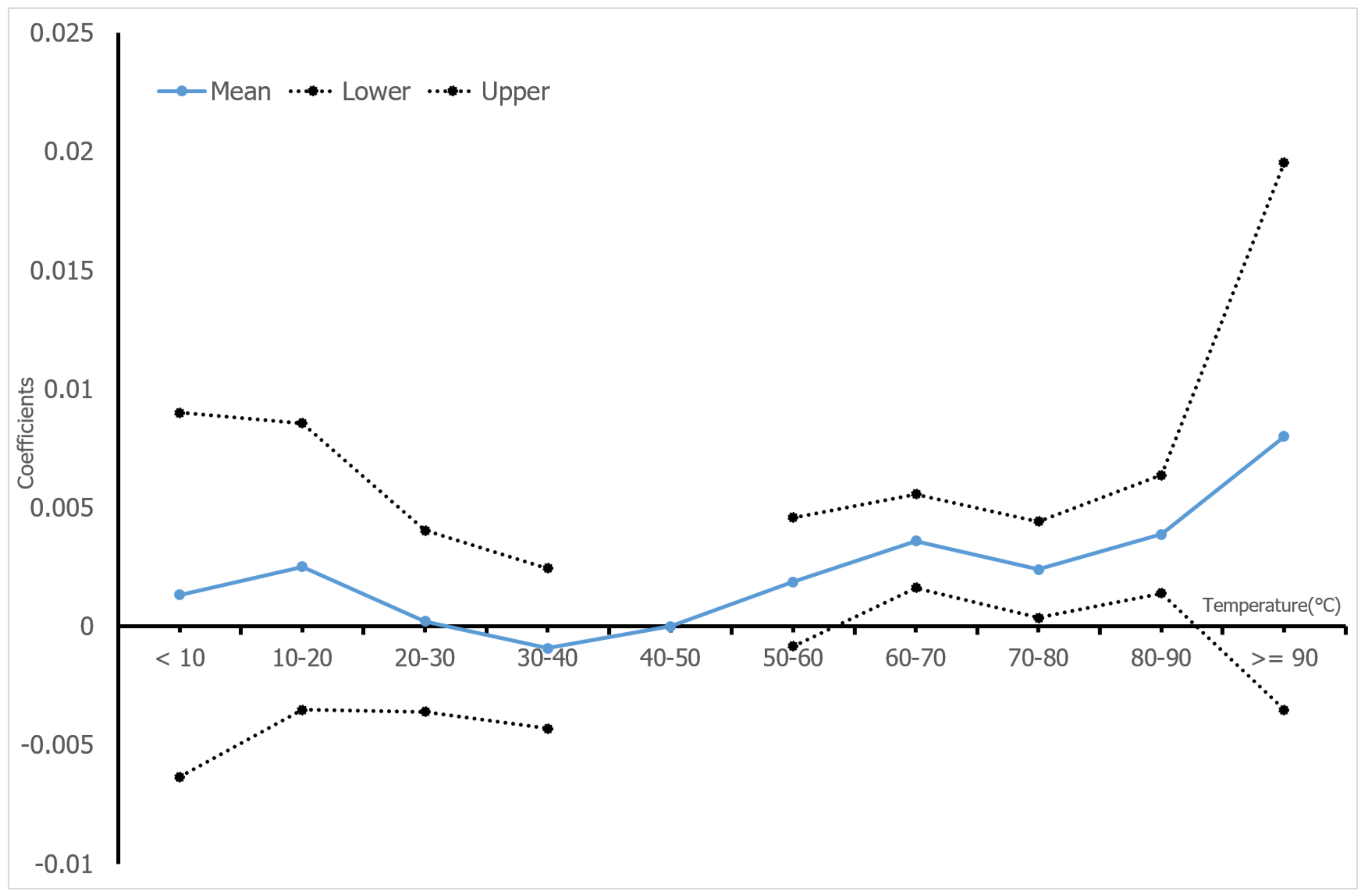
Figure 1 plots the estimates of temperature bins in the specification. Even though it shows the U-shaped curve, the coefficients below ‘–’ are not statistically significant. On the other hand, ‘–’ to ‘–’ have significantly positive responses. However, the hottest interval, ‘Days ’ does not have a statistically significant effect on fuel consumption because there are small observations and deviations for the temperature bin. Based on the results of (3), we estimate the same specifications, but drop below ‘–’ intervals. Therefore, the coefficients in (4) imply the relative response to ‘Days ’. Unlike the result of (3), the estimates in (4) have significant responses even though the magnitudes are similar.
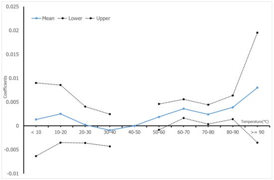
Figure 1.
Estimates of Impact of Weather on Fuel Consumption: Model 3.
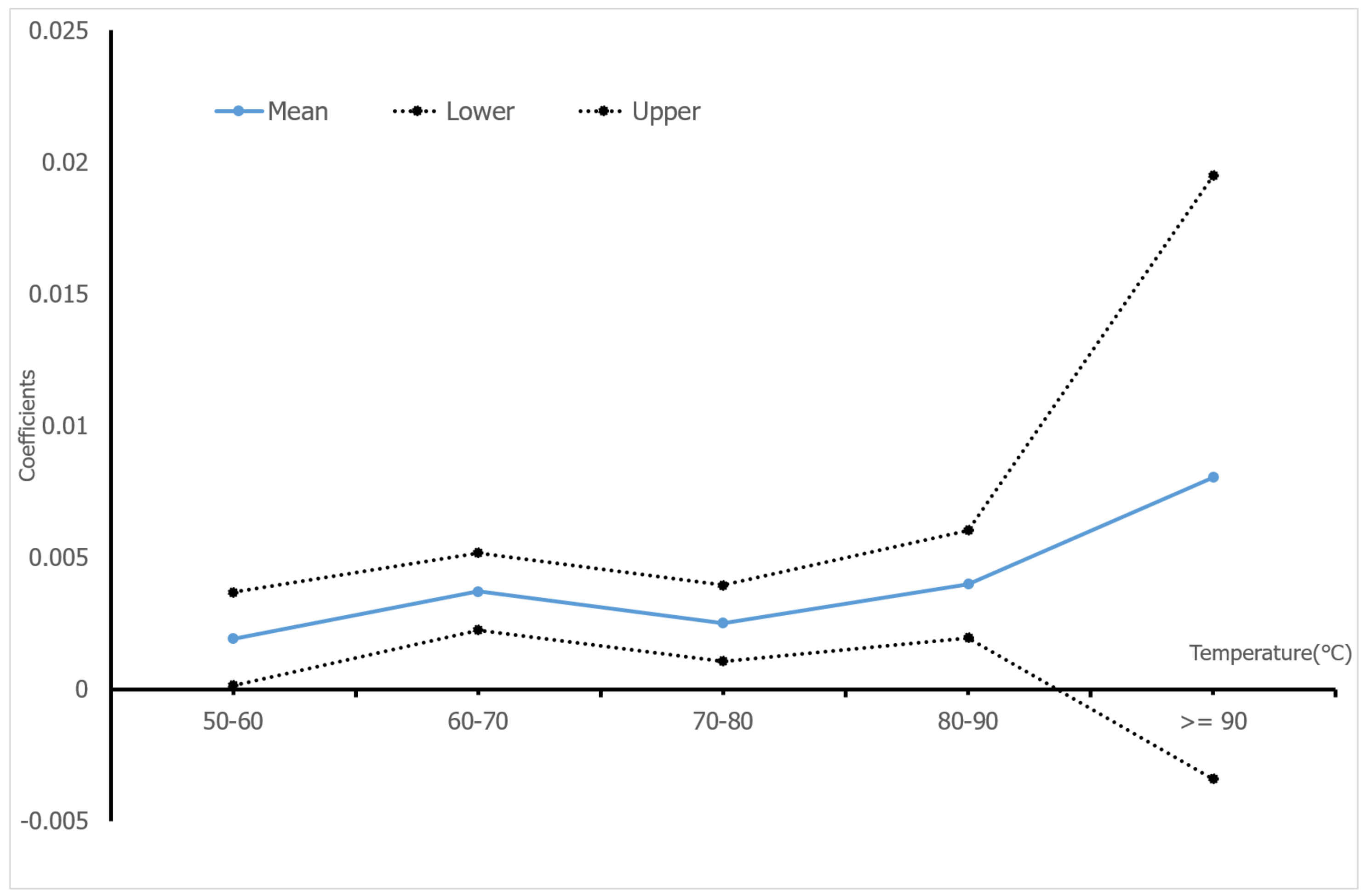
Figure 2 displays the coefficients for temperature responses. Similar to the coefficient for ‘Days ’ in (3), the estimate for the hottest interval in (4) has large confidence levels. Also, we estimate two types of disaggregated samples by region and income level.
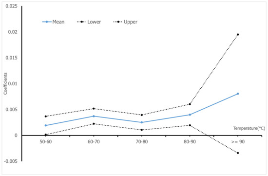
Figure 2.
Estimates of Impact of Weather on Fuel Consumption: Model 4.
Table 4 presents the regional specific estimates. The magnitudes and statistical significance vary with census regions. The coefficients for ‘Days –’ range from 0.0024 to 0.0058, but the estimate for Northeast is not statistically significant. Overall, only the South region has statistical precision as much as the whole sample, but other regions do not.
Table 4.
Estimation Results: Regional Specific Estimates.
Table 5 reports the estimates by income groups. We divide the households into three groups, lower, middle, and upper class within each year. As regional specific estimates, the coefficients vary with income level. Interestingly, the estimates for the high-income group are statically significant, but not for lower- and middle-income groups. The results imply that households with high income are more responsive to weather variations because they frequently use cooling equipment such as air conditioners while poor households occasionally do not use or buy it.
Table 5.
Estimation Results: Income-group Specific Estimates.
5.2. Simulation Results
To simulate the impact of climate change on fuel consumption, we build weather prediction data from two General Circulation Models (GCM), CCSM4 and GFDL-CM3. As implemented in the literature, we divide four different periods, 2020–2039, 2040–2059, 2060–2079, and 2080–2099. In addition, this study simulates based on two different climate change scenarios adopted in the IPCC Fifth Assessment Report (IPCC AR5), RCP 4.5 (stabilization without overshoot) and RCP 8.5 (rising). This study uses the simple equation used in [17] to measure the fuel consumption change by each climate change scenario
where and are the energy consumption for period t and , and are the number of the days belonging to temperature bin j for period t and . Equation (3) implies that the change in fuel consumption comes only from climate change without any other effects.
Table 6 presents the results based on Model 3 and Model 4 for each scenario, the GCM model, and period. The impact of climate change ranges from 0.56% (2020–2039, RCP 4.5 from CCSM4) to 8.58% (2080–2099, RCP 8.5 from GFDL-CM3). In comparison, the impact on residential energy consumption is up to 55% in [17] and 11% in [4]. It implies that the magnitude of climate change impact on passenger vehicle fuel consumption is relatively small. However, as we know from estimation results, fuel consumption in passenger vehicles is affected only in hot weather, while residential electricity has a positive impact from both hot and cold temperatures. In summer, under RCP 8.5 scenario, the climate change increase in fuel consumption goes up to around 20%.
Table 6.
Simulation of Climate Change Impacts.
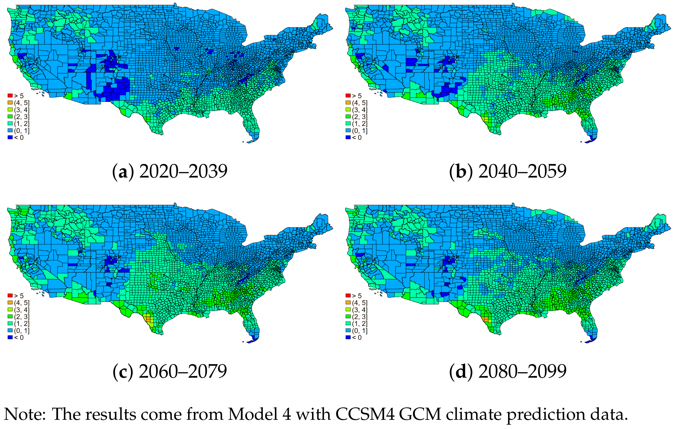
Figure 3 and Figure 4 show regional variations in the impact of climate change. Under the RCP 4.5 scenario, the impact is below 2% across the continental United States, even at the end of the century. However, most counties in the South region are expected to see greater than a 5% increase under RCP 8.5 scenario. In addition, most counties will have over a 3% increase in fuel consumption caused by climate change. It implies that the impact of climate change on gasoline consumption is heterogeneous locally.
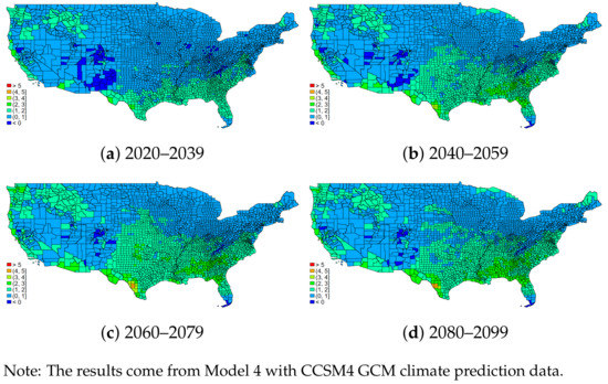
Figure 3.
Climate Change Simulation Results: RCP 4.5.

Figure 4.
Climate Change Simulation Results: RCP 8.5.
6. Conclusions and Policy Implications
A general contribution of the paper is to expand the existing evidence on the impact of climate change on energy consumption into the transportation sector, in particular, passenger vehicles. This study uses household-level panel data from the Panel Study of Income Dynamics (PSID) from 1999 to 2011. With panel household data, we estimate the fixed-effect model to solve omitted variable bias which is one of the main concerns in cross-section and time-series data. We investigate the relationship between temperature and fuel consumption with several different functional forms for temperature. In addition, with climate prediction data from GCMs, we simulate the impact of climate change on fuel energy consumption. The results have three main implications for the impact of climate change. First, hot days lead to higher fuel consumption, while cold days do not have a significant impact. In the literature on empirical evidence of the relationship between temperature and residential energy consumption, cold weather significantly increases energy consumption as well. Second, climate change increases fuel consumption by up to around 4% under “business-as-usual” (RCP 8.5) scenario. Even though the magnitude of the impact is less than in the residential energy consumption, the overall impact on greenhouse gas emission would be large because the transportation sector accounted for over 25% of greenhouse gas emissions in 2014, which is much larger than the residential sector. In addition, as mentioned above, fuel consumption in passenger vehicles is affected only by hot days. Therefore, the annual increase is relatively small while there is a larger effect in the summer season. Third, climate change has a heterogeneous impact across the continental United States. In particular, the impact in the South is bigger while the other regions are relatively small. However, our results cannot speak to all other regions or countries because the United States is the most car-dependent country in the world (https://stats.oecd.org/Index.aspx?DataSetCode=ITF{_}PASSENGER{_}TRANSPORT). It implies that the driver’s behavior in response to temperature changes can vary significantly. Moreover, since the purpose of this study is to consider only the net effects of climate change on gasoline consumption, we do not reflect technological improvements such as solar and biomass. It implies that the prediction results of this study are likely to be exaggerated.
Funding
This research project is financially supported by Korea Environment Industry & Technology Institute (KEITI) through Climate Change R&D program, funded by Korea Ministry of Environment (MOE) (2018001310001).
Conflicts of Interest
The authors declare no conflict of interest.
Abbreviations
| GCM | General Circulation Model |
| RCP | Representative Concentration Pathway |
| CDD | Cooling Degree Days |
| PRISM | Parameter-Elevation Regressions on Independent Slopes Model |
| NEX-GDDP | NASA Earth Exchange Global Daily Downscaled Projections |
| CCSM5 | Community Climate System Model5 |
| GFDL-CM3 | Geophysical Fluid Dynamics Laboratory Coupled Model3 |
| CMIP5 | Coupled Model Intercomparison Project Phase 5 |
| CAFE | Corporate Average Fuel Economy |
Appendix A
Appendix Sources of Data
- The Panel Study of Income Dynamic: http://simba.isr.umich.edu/data/data.aspx
- County-Level Gasoline Prices—ACCRA: https://www.coli.org
- EIA State-Level Gasoline Prices: http://www.eia.gov/petroleum
- EPA fuel economy: https://www.fueleconomy.gov
- NASA Earth Exchange Global Daily Downscaled Projections (NEX-GDDP): https://cds.nccs.nasa.gov/nex-gddp/
Appendix B
Table A1.
Estimation Results (Random-Effect Models).
References
- Deschênes, O.; Greenstone, M. The Economic Impacts of Climate Change: Evidence from Agricultural Output and Random Fluctuations in Weather. Am. Econ. Rev. 2007, 102, 3761–3773. [Google Scholar] [CrossRef]
- Schlenker, W.; Roberts, M.J. Nonlinear temperature effects indicate severe damages to U.S. crop yields under climate change. Proc. Natl. Acad. Sci. USA 2009, 106, 15594–15598. [Google Scholar] [CrossRef] [PubMed]
- Auffhammer, M.; Aroonruengsawat, A. Simulating the impacts of climate change, prices and population on California’s residential electricity consumption. Clim. Chang. 2011, 109, 191–210. [Google Scholar] [CrossRef]
- Deschênes, O.; Greenstone, M. Climate change, mortality, and adaptation: Evidence from annual fluctuations in weather in the US. Am. Econ. J. Appl. Econ. 2011, 3, 152–185. [Google Scholar] [CrossRef]
- Xu, P.; Huang, Y.J.; Miller, N.; Schlegel, N.; Shen, P. Impacts of climate change on building heating and cooling energy patterns in California. Energy 2012, 44, 792–804. [Google Scholar] [CrossRef]
- Auffhammer, M.; Baylis, P.; Hausman, C.H. Climate change is projected to have severe impacts on the frequency and intensity of peak electricity demand across the United States. Proc. Natl. Acad. Sci. USA 2017, 114, 201613193. [Google Scholar] [CrossRef]
- Auffhammer, M.; Mansur, E.T. Measuring climatic impacts on energy consumption: A review of the empirical literature. Energy Econ. 2014, 46, 522–530. [Google Scholar] [CrossRef]
- Eisenberg, D.; Warner, K.E. Effects of Snowfalls on Motor Vehicle Collisions, Injuries, and Fatalities. Am. J. Public Health 2005, 95, 120–124. [Google Scholar] [CrossRef]
- Leard, B.; Roth, K. Weather, Trafiic Accidents, and Climate Change. J. Clim. 1993, 759–767. [Google Scholar] [CrossRef]
- Weitzman, M.L. Fat-Tailed Uncertainty in the Economics of Catastrophic Climate Change. Rev. Environ. Econ. Policy 2011, 5, 275–292. [Google Scholar] [CrossRef]
- Yuksel, T.; Michalek, J.J. Effects of regional temperature on electric vehicle efficiency, range, and emissions in the united states. Environ. Sci. Technol. 2015, 49, 3974–3980. [Google Scholar] [CrossRef] [PubMed]
- Engle, R.F.; Granger, C.W.J.; Rice, J.; Weiss, A. Semiparametric Estimates of the Relation Between Weather and Electricity. J. Am. Stat. Assoc. 1986, 81, 310–320. [Google Scholar] [CrossRef]
- Chang, Y.; Kim, C.S.; Miller, J.I.; Park, J.Y.; Park, S. Time-varying Long-run Income and Output Elasticities of Electricity Demand with an Application to Korea. Energy Econ. 2014, 46, 334–347. [Google Scholar] [CrossRef]
- Vaage, K. Heating technology and energy use: A discrete continuous choice approach to Norwegian household energy demand. Energy Econ. 2000, 22, 649–666. [Google Scholar] [CrossRef]
- Mansur, E.T.; Mendelsohn, R.; Morrison, W. Climate change adaptation: A study of fuel choice and consumption in the US energy sector. J. Environ. Econ. Manag. 2008, 55, 175–193. [Google Scholar] [CrossRef]
- Dubin, J.A.; Mcfadden, D.L. An Econometric Analysis of Residential Electric Appliance Holdings and Consumption. Econometrica 1984, 52, 345–362. [Google Scholar] [CrossRef]
- Auffhammer, M.; Kellogg, R. Clearing the air? the effects of gasoline content regulation on air quality. Am. Econ. Rev. 2011, 101, 2687–2722. [Google Scholar] [CrossRef]
- Tack, J.; Harri, A.; Coble, K. More than Mean Effects: Modeling the Effect of Climate on the Higher Order Moments of Crop Yields. Am. J. Agric. Econ. 2012, 94, 1037–1054. [Google Scholar] [CrossRef]
- Auffhammer, M.; Hsiang, S.M.; Schlenker, W.; Sobel, A. Using Weather Data and Climate Model Output in Economic Analyses of Climate Change. Rev. Environ. Econ. Policy 2013, 7, 181–198. [Google Scholar] [CrossRef]
- Franco, G.; Sanstad, A.H. Climate change and electricity demand in California. Clim. Chang. 2007, 87, 139–151. [Google Scholar] [CrossRef]
- Considine, T.J. The impacts of weather variations on energy demand and carbon emissions. Resour. Energy Econ. 2000, 22, 295–314. [Google Scholar] [CrossRef]
- Fan, S.; Hyndman, R.J. The price elasticity of electricity demand in South Australia. Energy Policy 2011, 39, 3709–3719. [Google Scholar] [CrossRef]
- Chang, Y.; Kim, C.S.; Miller, J.I.; Park, J.Y.; Park, S. A New Approach to Modeling the Effects of Temperature Fluctuations on Monthly Electricity Demand. Energy Econ. 2016, 60, 206–216. [Google Scholar] [CrossRef]
- Thrasher, B.; Maurer, E.P.; McKellar, C.; Duffy, P.B. Technical Note: Bias correcting climate model simulated daily temperature extremes with quantile mapping. Hydrol. Earth Syst. Sci. 2012, 16, 3309–3314. [Google Scholar] [CrossRef]
- Frondel, M.; Ritter, N.; Vance, C. Heterogeneity in the rebound effect: Further evidence for Germany. Energy Econ. 2012, 34, 461–467. [Google Scholar] [CrossRef]
- Cameron, A.C.; Trivedi, P.K. Microeconometrics Using Stata; Stata Press: College Station, TX, USA, 2010. [Google Scholar]
- Sorrell, S.; Dimitropoulos, J.; Sommerville, M. Empirical estimates of the direct rebound effect: A review. Energy Policy 2009, 37, 1356–1371. [Google Scholar] [CrossRef]

© 2019 by the author. Licensee MDPI, Basel, Switzerland. This article is an open access article distributed under the terms and conditions of the Creative Commons Attribution (CC BY) license (http://creativecommons.org/licenses/by/4.0/).