Abstract
In the transition to a low-carbon economy, climate-resilient investors may be inclined to buy renewable-energy or other low-carbon assets. As the diversification benefits of investment positions in those assets depend on interdependence between their market prices, we explore that interdependence in the European and USA stock markets. We model the dependence structure using bivariate copula functions and evaluate price spillovers between those markets using a conditional quantile dependence approach that accounts for the reciprocal effects of price movements in those markets under normal and extreme market scenarios. Our empirical evidence for the period 2010–2019 indicates that European renewable-energy and low-carbon stocks co-move; upward and downward movements in low-carbon asset prices have sizeable effects on renewable-energy asset prices, and vice versa, although effects are smaller. In contrast, for the USA we find evidence of non-interdependence, with no significant upward or downward price spillover effects between renewable-energy and low-carbon stocks. Our empirical findings provide useful insights for the design of carbon-resilient portfolios and risk management strategies, and also for implementation of public funding policies to support the transition to a low-carbon economy.
JEL Classification:
C22; C58; F30; G11; G15
1. Introduction
The transition to a low-carbon economy entails a vast amount of financial resources, which, in turn, raises awareness among investors about opportunities and risks linked to that transition. Renewable-energy and low-carbon assets are arguably the most suitable investment vehicles to ensure private capital reallocation that meets the challenges posed by decarbonization. Therefore, understanding interdependence between the prices of renewable-energy and low-carbon assets is essential information for environmentally-friendly investors, as it determines the diversification benefits of allocating private capital to climate-resilient portfolios and shapes private incentives to deploy financial resources to clean energies and low-carbon industries. Moreover, interdependence between renewable-energy and low-carbon assets is also of interest for policymakers, as low-carbon investments could provide adequate incentives to invest in renewable energies and vice versa, thereby determining public funds to be allocated to support the transition to a climate-resilient economy.
We examine dependence between renewable-energy and low-carbon stock prices using a conditional quantile price dependence approach that allows price spillovers between those markets to be explored under different market circumstances, including extreme upward and downward movements in asset values ([1]). Specifically, to assess the impact of price movements of a particular size in one market on stock prices in the other market, we characterize the bivariate dependence structure between renewable-energy and low-carbon stock price returns through copulas, then we compute conditional stock return quantiles and evaluate whether these differ from unconditional quantiles.
The extant literature on renewable-energy and low-carbon stock prices has developed along two separate strands.
One strand has examined the relationship between clean-energy and oil prices. Some studies have explored causality between oil prices and renewables, finding evidence of Granger causality that differs across sample periods and time horizons ([2,3,4,5,6]). Other studies have examined oil price spillovers to renewable stocks, documenting significant impacts from oil price oscillations to renewable stock prices ([7,8,9]), volatility spillovers between oil and clean-energy stocks ([10,11,12]) and connectedness between clean energy stocks, oil prices and financial variables ([13]). Likewise, a different set of articles have explored dynamic correlations between renewable energy and stock prices ([14]) and the contribution of energy prices to renewable asset prices and volatility ([15,16,17]).
The other strand has investigated the effects of carbon emissions on firm performance and on investor portfolios. The authors of [18] find that firm value is negatively impacted by carbon emissions, whereas [19] shows that the cost of capital increases with carbon emissions. The authors of [20,21] find that firms with higher carbon emissions earn higher returns, whereas [22] show that higher emissions are related with higher levels of downside risk. From an investor’s perspective, the authors of [23] explores a dynamic investment strategy for passive investors to hedge climate risk without sacrificing financial returns, finding that, even for low-carbon indexes with carbon footprints of 50% less than the benchmark, the tracking error can be virtually eliminated; they also indicate that those results could improve with the pricing of carbon dioxide emissions. Similarly, the authors of [24] shows how bond investor portfolios can be hedged against climate risk with no introduction of unintended exposure that could sacrifice a portfolio’s benchmark-tracking properties. More recently, in their investigation of investor portfolio divestment from fossil fuels, the authors of [2] find that clean-energy investments offer better returns, whereas [25], in comparing the financial performance of investment portfolios with and without fossil fuel stocks, report that fossil fuel divestment does not seem to impair portfolio performance, given that fossil fuel stocks do not outperform other stocks on a risk-adjusted basis and that fossil fuel stocks provide relatively limited diversification benefits. Likewise, the authors of [26] contend that socially responsible investing has not been costly in terms of forgone market returns, as the return performance of a fossil-fuel-free portfolio surpasses the S&P 500 returns index due to poor fossil fuel sector performance.
From the investors’ perspective, the above-mentioned strands in the literature provide useful information on the impact of energy prices or carbon emissions on the value of low-carbon portfolios composed of either renewable energy or low-carbon assets. However, this literature is silent about the impact of changes in low-carbon asset values on renewable energy asset values and vice versa; such information is crucial for climate-friendly investors as both renewable-energy and low-carbon assets are alternative or complementary assets in terms of the design and risk diversification aims of low-carbon portfolios. This paper fills this gap by analysing interdependence between renewable-energy and low-carbon stock prices in a bivariate copula framework and computing how differently sized stock price movements in one market impact on stock prices in the other market. We model price changes in renewable-energy and low-carbon assets using a multifactor pricing model that includes autoregressive components, with co-movement under different market circumstances modelled through copulas taking into account the effect of common pricing factors in that co-movement. Our empirical study covers the period January 2010 to July 2019 and the European and the USA markets, with renewable-energy stocks represented by the European Renewable Energy and the Wilder Hill Clean Energy indexes, respectively, and low-carbon assets represented by the Euro STOXX Low Carbon Select 50 and the USA STOXX Low Carbon Select 50 indexes, respectively. Our empirical results point to dissimilarities in both stock markets. Specifically, while we observe interdependence between renewable-energy and low-carbon markets in Europe, those markets do not co-move in the USA. Furthermore, we find evidence of symmetric tail dependence in Europe but independence in the USA. We consistently find evidence of symmetric downside and upside price spillover effects between the European renewable-energy and low-carbon stock markets, differing, however, in that price spillovers from low-carbon to renewable-energy stocks are greater than vice versa. Contrarily, for the USA, we find no evidence of price spillovers.
These findings have implications for both investors and policymakers. Investors holding positions in renewables can hedge such positions using low-carbon assets when they invest in the USA market but should seek alternative hedging devices for the European market. As low-carbon and renewable-energy stocks in the European markets behave as a similar asset class, raising funds for renewables from environmentally-aware investors is more difficult as there are opportunities to invest in other low-carbon assets. Finally, our evidence is informative for the design and funding of renewable energy policies: boosting funding to renewables may have a detrimental effect on low-carbon industries in Europe but only a minor effect in the USA.
The remainder of the paper is laid out as follows. In Section 2 we outline our methodology to assess conditional quantile dependence using copula functions. In Section 3 we describe the main features of our data for renewable-energy and low-carbon stock markets in Europe and the USA. In Section 4 we discuss our results on dependence, the impact of price oscillations from/to low-carbon assets and to/from renewable-energy stocks, and the main implications of those results. Finally, Section 5 summarizes our results and concludes this study.
2. Empirical Methods
2.1. Quantile Dependence between Renewable-Energy and Low-Carbon Markets
We measure price impacts between the renewable-energy and low-carbon markets using the quantile copula dependence approach developed by [1], which allows the impact of quantile price changes between markets to be assessed. The use of bivariate copula models offers modeling flexibility in featuring bivariate distribution functions, as copulas account for particular data characteristics in the marginal distribution functions, such as time-varying volatilities or leverage effects, and they allow dependence to differ under different market circumstances, in particular in times of extreme price oscillations.
To begin with, using copulas rather than quantile regression results in greater modeling flexibility; this is because copulas enable heterogeneity in characterizing marginal distributions and also account for specific data features such as conditional heteroskedasticity, volatility asymmetries, and leverage effects. Moreover, our empirical setup allows for time-varying dependence, so the impact of oil price changes on stock returns are allowed to differ in different moments of time depending on the dependence and volatility features of the corresponding markets.
Let re and be the (log) change in prices of renewable-energy and low-carbon stocks, respectively. The impact of a change in the price of a low-carbon asset of a size given by its -quantile on the -quantile of the renewable-energy market can be measured by the conditional -quantile of the renewable return distribution at time t, , as:
where is the unconditional -quantile of the low-carbon price returns distribution: . From this conditional quantile, we can quantify how price fluctuations in low-carbon stocks of different sizes impact on renewable-energy stocks under different market scenarios as reflected by the quantiles of low-carbon stocks. Similarly, we can obtain the reverse impact, i.e., the impact of price fluctuations in renewable-energy stock prices on the prices of low-carbon assets.
From [27]’s theorem on equality between the joint distribution function and a copula function C, we can express Equation (1) in terms of the joint distribution function or the copula function as:
where and denote the marginal distribution functions for the renewable-energy and low-carbon price changes, respectively and where the second equality follows from the fact that the joint distribution is the product of the conditional and marginal distributions, , with and . Hence, for given values for and and for the copula model specification, we can compute by inverting the copula function in Equation (2), , in order to obtain the value of ; then, by inverting the marginal distribution function of we obtain the conditional quantile as:
Note that if renewable-energy and low-carbon stock markets are independent, then , so . Hence, the difference between conditional and unconditional renewable-energy return quantiles provides information on the impact of low-carbon stock price changes on renewable-energy stock returns.
To compute the conditional quantile through copulas we need information on the marginal distribution models and on dependence between renewable-energy and low-carbon market prices as given by the copula function. Using copulas rather than the conditional marginal distribution to compute conditional quantiles has the appeal of flexibility, in that copulas separate modeling of the marginals and of the dependence structures, and they capture dependence in the case of sharp upward (upper quantiles) or downward (lower quantiles) price movements.
2.2. Marginal and Copula Models
As the mean and variance of financial return series exhibit time-varying behavior and stock returns depend on general pricing factors, we estimate the price dynamics of renewable-energy and low-carbon stocks using an autoregressive moving average (ARMA) model with p and q lags and with exogenous variables as given by the five pricing factors proposed by [28,29]:
where denotes the excess price returns in renewable-energy and low-carbon stocks and where the pricing factors are as follows: is the excess return of the market portfolio; is the difference between the returns of a diversified portfolio comprised of small and large assets; is the difference between high book-to-market and low book-to-market portfolio returns; is the difference between returns for a diversified portfolio of robust and weak profitability assets; and is the difference between portfolio returns for low (conservative) and high (aggressive) investment firms. is a stochastic component with zero mean and variance , which has a dynamic described by a threshold generalized autoregressive conditional heteroskedasticity (TGARCH) model:
where is a constant parameter and where the parameters and account for the generalized autoregressive conditional heteroskedasticity (GARCH) and autoregressive conditional heteroskedasticity (ARCH) effects, respectively. for , then the parameter captures asymmetric effects: when () negative shocks have more (less) impact on variance than positive shocks (note that for we have symmetric effects as given by the GARCH model). Fat tails and asymmetries of the stochastic component , and thus of , are captured by [30] skewed-t density distribution; this distribution is characterized by parameters v (the degrees-of-freedom parameter, ) and (the symmetric parameter, ).
We model dependence by considering different copula specifications for the variables x and y, with and . Specifically, we capture positive and negative dependence using the bivariate Gaussian copula, given by , where is the bivariate standard normal cumulative distribution function with correlation and where and are standard normal quantile functions. Similarly, positive and negative dependence is captured by the student-t copula, which is given by , where is the bivariate student-t cumulative distribution function with the degree-of-freedom parameter v and dependence given by the correlation coefficient and where and are the quantile functions of the univariate student-t distribution. Gaussian and student–t copulas differ in terms of their tail dependence: the former exhibit zero tail dependence while the latter show symmetric tail dependence and converge to the Gaussian when the degrees of freedom go to infinity. We also consider the Gaussian and student-t copulas with time-varying parameters, with a dynamic given by [31]:
where is the modified logistic transformation that retains in (−1,1). As for the student-t copula, is replaced by . We also use the symmetric Plackett copula, which, like the Gaussian copula, exhibits tail independence although it displays more dependence for large joint realizations. It is given by:
Furthermore, we capture asymmetric dependence using the Gumbel copula, given by , which has upper tail dependence and lower tail independence. Moreover, we rotate the Gumbel copula 180° with parameter : . Finally, we also consider time-varying dynamics of the dependence parameter as given by:
Finally, the parameters of the marginal and copula models are estimated using the inference function for margins ([32]), which allows parameter estimation in two steps. First, the parameters of the marginal models are first estimated using maximum likelihood. Next, the copula parameters are estimated by maximum likelihood using, as pseudo-sample observations for the copulas, the probability integral transformation of the standardized residuals from the marginals. The number of lags in the mean and variance equations in the marginal models are selected using the Akaike information criteria (AIC), whereas the adequate copula specification is selected using the AIC adjusted for small-sample bias ([33]).
3. Data
Our empirical analysis on quantile dependence between renewable-energy and low-carbon stocks in the European and USA stock markets is based on the respective stock market indices. Specifically, we consider the Europe STOXX Low Carbon Select 50 Index (LC-EU) and the USA STOXX Low Carbon Select 50 Index (LC-USA) for the European and USA stock markets, respectively. These indices, which exclude all companies involved in the coal sector, capture the performance of low carbon emissions stocks with low volatility and high dividends selected from the universe of companies included in the STOXX Europe 600 Index and in the STOXX Global 1800 index, respectively. The 50 assets included in the index are weighted according to the inverse of their volatility, with a cap at 10%, and the index is reviewed quarterly.
To account for the performance of renewable-energy stocks, we take the European Renewable Energy index (ERIX) and the Wilder Hill Clean Energy index (ECO) for Europe and USA, respectively. ERIX is comprised of the largest European renewable-energy companies with wind, solar, biomass, and water energy generation as their main activities. ECO is an equal-dollar-weighted index of a set of companies that develop activities related to clean energies and conservation.
The sample covered the period 1 January 2010 to 31 July 2019, with the start date of the sample period determined by the availability of data for low-carbon indices. Data was sourced from Bloomberg on a daily basis. Figure 1 displays the temporal dynamics of renewable-energy and low-carbon markets in the European and USA markets, showing that these markets follow similar trends, with price changes harmonized in Europe, but not synchronized in the USA. We computed daily price returns as the first difference for the (log) value of those indices. Table 1 presents the main statistical features of the daily returns. For all markets under study, average daily returns are close to zero and standard deviations are greater for the renewable-energy stocks than for the low-carbon stocks. Higher volatility in renewable-energy markets is also confirmed by the maximum and minimum values of returns. All price returns exhibit negative skewness and the price return distributions have fat tails. In fact, the Jarque–Bera (JB) test rejects normality. The evidence of serial dependence provided by the Ljung–Box (LJ) statistic is mixed: although most of the series exhibit serial independence, low-carbon series for Europe show serial dependence. Finally, the ARCH test points to the presence of conditional heteroskedasticity in the series.
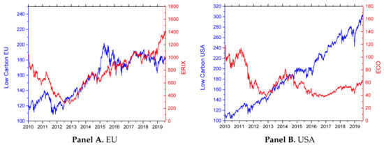
Figure 1.
Time series plot for daily renewable-energy and low-carbon indices.

Table 1.
Descriptive statistics for renewable-energy and low-carbon indices.
Data for the pricing factors and the risk-free interest rates to compute excess returns in renewable-energy and low-carbon markets in Europe and the USA were sourced from the Kenneth French data library (http://mba.tuck.dartmouth.edu/pages/faculty/ken.french/data_library.html). Table 2 presents descriptive statistics for those pricing factors in both markets, showing that their behaviors differ across stock markets.
Table 2.
Descriptive statistics for pricing factors.
4. Empirical Evidence
4.1. Results for Marginal and Copula Models
Parameter estimates and goodness-of-fit tests for the marginal models for renewable-energy and low-carbon indices in the EU and the USA are presented in Table 3. We selected suitable lags for the mean and variance by considering lag values between 0 and 2, taking as the optimal values those that minimized the AIC. Our estimates reflect serial dependence in all price return series, given the significant autoregressive and moving average coefficients. Parameter estimates for the pricing factors indicate that all return series are dependent on the market factor, with betas below one indicating that renewable-energy and low-carbon stocks are defensive stocks, with the exception of the ECO index. However, we find mixed evidence for the remaining pricing factors as the significance of those factors differs across markets. Likewise, parameter estimates for the volatility dynamics indicate that volatility displays persistence and no leverage effects, with the exception of the European low-carbon market. The degrees-of-freedom parameter also indicates that the error terms are generally symmetric and exhibit fat tails, whereas asymmetry is significant in the low-carbon markets.
Table 3.
Maximum likelihood estimates.
The last six columns of Table 3 show results for goodness-of-fit tests for the estimated marginal models. The LJ test indicates that there is no serial correlation in either the residual series or the squared residual series, and the ARCH-Lagrange multiplier (ARCH-LM) statistic indicates that no GARCH effects remain in the model residuals. In comparing the empirical and theoretical distribution functions of the standardized residuals, the Kolmogorov–Smirnov (KS), Cramér–von Mises (CVM), and Anderson–Darling (AD) tests all support the null hypothesis of correct specification of the distribution models for all the series.
We estimate copula model parameters using the probability integral transform of the standardized residuals from the estimated marginal models as pseudo-sample observations for the copula. Parameter estimates for the static and time-varying copulas are reported in Table 4. Empirical estimates point to relevant difference between the European and USA markets. Thus, while in the European market we find evidence of positive dependence between renewable-energy and low-carbon stock markets, for the USA we find that this dependence to be negative and small. Evidence on comparing copulas through the AIC values indicates that the static student-t copula provides the best fit for the European markets and the Plackett copula for the USA market. Furthermore, dependence between renewable-energy and low-carbon stock markets is fundamentally static. We only find evidence of tail dependence in the European market, so upward or downward movements in renewable-energy stock prices have impacts on the low-carbon market and vice versa. In contrast, for the USA market we find evidence of no tail dependence and weak negative average dependence, so abrupt price changes in renewable-energy stock prices have negligible effects on low-carbon assets and vice versa.
Table 4.
Estimates for the copula models.
4.2. Price Impact Results for the Renewable-Energy and Low-Carbon Stock Markets
We estimate conditional quantiles using information from the estimated marginal and copula models, taking different values for the quantiles and given by 0.05, 0.10, 0.25, 0.5, 0.75, 0.9, and 0.95. To assess the relative impact of low-carbon stock prices on renewable-energy prices and vice versa, we also estimate the unconditional quantiles from the marginal models as for and and are given by the ARMA and GARCH components of the marginal model, with denoting the value of the -quantile of the skewed student-t distribution.
Figure 2 depicts the quantile dynamics of the upper and lower conditional and unconditional renewable quantiles in the European and the USA markets, considering the impact of high (low) price fluctuations in low-carbon stocks as given by the 0.9 (0.1) quantile on the high (low) renewable-energy quantile as given by the 0.9 (0.1) quantile. Consistent with the evidence on tail dependence in the European renewable-energy stock market, we found that differences between conditional and unconditional quantiles in the upper and lower tails of the joint distribution were sizable and of a similar size. Hence, sharp upward or downward movements in low-carbon stocks have an impact on prices of renewable-energy stocks in the European markets. However, this effect is not observed in the USA market, as there is near zero dependence, i.e., the impact of price oscillations in low-carbon assets has no sizeable impact on renewable-energy stock prices, as reflected in Panel B of Figure 2.
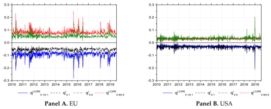
Figure 2.
Temporal dynamics for upper and lower conditional and unconditional quantiles of renewable-energy stock returns.
As for the impact of price oscillations in renewable-energy stocks on low-carbon stock prices, Figure 3 depicts upper and lower conditional and unconditional low-carbon quantiles in the European and the USA markets, considering the impact of high (low) price fluctuations in renewable-energy stocks as given by the 0.9 (0.1) quantile on the high (low) low-carbon quantile as given by the 0.9 (0.1) quantile. Graphical evidence reflects that price impacts differ in both stock markets; in the European market, price movements in renewable-energy stocks have a significant impact on low-carbon stock prices, whose impact is smaller than in reverse, whereas in the USA market—consistently with near independence—differences between conditional and unconditional quantiles are small.
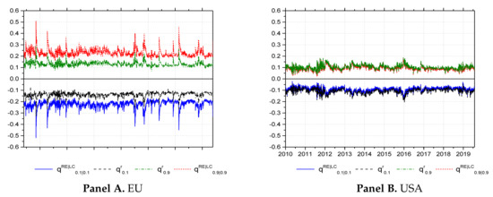
Figure 3.
Temporal dynamics for upper and lower conditional and unconditional quantiles of low-carbon stock returns.
Finally, Figure 4 and Figure 5 summarize the relative impact of price changes in low-carbon assets of specific sizes on renewable-energy stocks and vice versa, respectively. For different values, the plots represent the average value of the conditional quantile over the unconditional quantile: values greater than one, depicted in warm colours, indicate that stock price changes in one market affect the corresponding unconditional quantile of the other market, whereas values in cold colours indicate the opposite. For the European markets, Panel A in Figure 4 and Figure 5 confirms that renewables and low carbon markets closely co-move, so upward or downward movements in one of the markets have a positive and significant effect on the prices in the other market. Likewise, graphical evidence also corroborates that opposite movements in renewable-energy and low-carbon prices are not related, consistent with the idea that markets move in tandem. In contrast, for the US, graphical evidence in Panel B reflects the fact that renewable-energy and low-carbon markets move independently, i.e., price changes in one market are not reflected in price movements in the other market as indicated by the equality between conditional and unconditional quantiles.
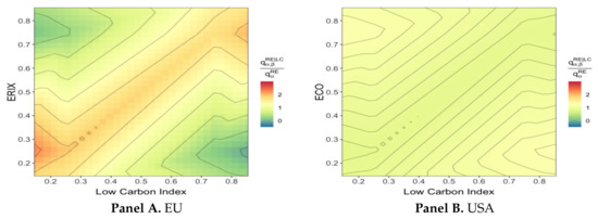
Figure 4.
Average value of conditional over unconditional quantiles for renewable-energy stocks.
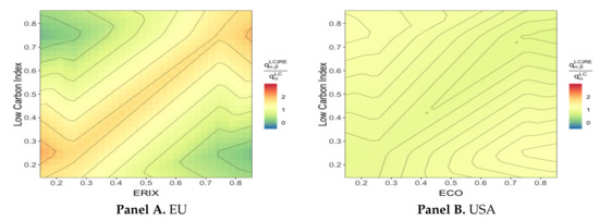
Figure 5.
Average value of conditional over unconditional quantiles for low-carbon stocks.
5. Conclusions
Investing in renewable-energy and low-carbon assets is a straightforward way for investors to align their portfolios with a low-carbon and more climate-resilient economy. However, the diversification benefits of holding positions in such firms closely depends on the way both kinds of assets co-move. Climate-friendly investors could take advantage of this information to build more adequate portfolio investment strategies. We therefore explored interdependence between prices of renewable-energy and low-carbon assets in the European and USA stock markets for the period 2010–2019. We use copula functions, which report information on dependence under different market circumstances, even though we have no information on the causality effects.
Our empirical evidence documents that European, but not USA, renewable-energy and low-carbon markets co-move and, likewise, we find evidence of symmetric tail dependence in Europe but tail independence in the USA. Consistently, we find that upside or downside movements in the prices of low-carbon assets impact on renewable-energy asset prices in Europe, while the reverse is also notable, although smaller in size. In contrast, for the USA market we find that the impact of upward or downward price oscillations in low-carbon asset prices on the price of renewable-energy stocks is not sizable as is the case with the reverse.
Our empirical findings have practical implications for investor decision-making and for policy-makers as follows. First, evidence of positive co-movement between renewable-energy and low-carbon asset prices in Europe indicates that, as both kind of assets move in the same direction under different market scenarios, long positions in low-carbon assets cannot be hedged using long positions in renewable-energy assets, and vice versa. In the USA market, in contrast, since renewable-energy and low-carbon stock prices move independently, investors in either market could use one set of assets to hedge financial positions in the other market. Second, in Europe, climate-friendly investors cannot use renewable-energy assets to manage downside risks for long positions in low-carbon assets, and vice versa, unlike investors in the USA. Third, our evidence on interdependence between renewable-energy and low-carbon asset prices is useful for the design of energy policies to support and fund renewable energy investments. Specifically, when renewable-energy and low-carbon asset prices co-move—as happens in the European markets—public funding of renewables impact on renewable-energy companies, and this impact leads to price externalities for low-carbon companies. Likewise, the withdrawal of support policies for renewable energies (such as subsides) will have negative effects on the price of renewable-energy stocks that will be transmitted to the price of low-carbon assets. As a result, policy decisions regarding energy transition to a decarbonized economy should take into account the effects on low-carbon companies, as also crucial in the transition to a climate-resilient economy. However, when low-carbon and renewable-energy markets move independently—as happens in the USA—such policy effects are irrelevant. Finally, in raising funds for the transition to a low-carbon economy, the dependence between climate-friendly assets such as renewable-energy and low-carbon stocks is such as to render them a similar asset class; therefore, funds for renewable energies face competition in the demand for funds for other low-carbon industries that may also be attractive to environmentally friendly investors—the case in Europe; in the USA, however, the independence of the asset classes may spur investment incentives in climate-friendly assets such as renewable-energy and low-carbon stocks.
Author Contributions
Conceptualization, J.C.R., A.U., Y.C.; Methodology, J.C.R., A.U.; Data collection, A.U., Y.C., Estimation, A.U., Y.C.; Writing—Original Draft Preparation, J.C.R.; Review & Editing, J.C.R., A.U., Y.C.; Funding Acquisition, J.C.R., A.U.
Funding
Financial support from the Agencia Estatal de Investigación (Ministerio de Ciencia, Innovación y Universidades) is acknowledged for research project RTI2018-100702-B-I00, co-funded by the European Regional Development Fund (ERDF/FEDER). Juan C. Reboredo acknowledges funding from the Xunta de Galicia for research project CONSOLIDACIÓN 2019 GRC GI-2060 Análise Económica dos Mercados e Institucións—AEMI (ED431C 2019/11). Andrea Ugolini acknowledges financial support from the Brazilian National Council for Scientific and Technological Development (CNPq).
Conflicts of Interest
The authors declare no conflict of interest.
References
- Reboredo, J.C.; Ugolini, A. Quantile dependence of oil price movements and stock returns. Energy Econ. 2016, 54, 33–49. [Google Scholar] [CrossRef]
- Henriques, I.; Sadorsky, P. Investor implications of divesting from fossil fuels. Glob. Financ. J. 2018, 38, 30–44. [Google Scholar] [CrossRef]
- Managi, S.; Okimoto, T. Does the price of oil interact with clean energy prices in the stock market? Jpn. World Econ. 2013, 27, 1–9. [Google Scholar] [CrossRef]
- Kumar, S.; Managi, S.; Matsuda, A. Stock prices of clean energy firms, oil and carbon markets: A vector autoregressive analysis. Energy Econ. 2012, 34, 215–226. [Google Scholar] [CrossRef]
- Broadstock, D.C.; Cao, H.; Zhang, D. Oil shocks and their impact on energy related stocks in China. Energy Econ. 2012, 34, 1888–1895. [Google Scholar] [CrossRef]
- Reboredo, J.C.; Rivera-Castro, M.A.; Ugolini, A. Wavelet-based test of co-movement and causality between oil and renewable energy stock prices. Energy Econ. 2017, 61, 241–252. [Google Scholar] [CrossRef]
- Inchauspe, J.; Ripple, R.D.; Trück, S. The dynamics of returns on renewable energy companies: A state-space approach. Energy Econ. 2015, 48, 325–335. [Google Scholar] [CrossRef]
- Reboredo, J.C. Is there dependence and systemic risk between oil and renewable energy stock prices? Energy Econ. 2015, 48, 32–45. [Google Scholar] [CrossRef]
- Bondia, R.; Ghosh, S.; Kanjilal, K. International crude oil prices and the stock prices of clean energy and technology companies: Evidence from non-linear cointegration tests with unknown structural breaks. Energy 2016, 101, 558–565. [Google Scholar] [CrossRef]
- Sadorsky, P. Correlations and volatility spillovers between oil prices and the stock prices of clean energy and technology companies. Energy Econ. 2012, 34, 248–255. [Google Scholar] [CrossRef]
- Sadorsky, P. Modeling renewable energy company risk. Energy Policy 2012, 40, 39–48. [Google Scholar] [CrossRef]
- Wen, X.; Guo, Y.; Wei, Y.; Huang, D. How do the stock prices of new energy and fossil fuel companies correlate? Evidence from China. Energy Econ. 2014, 41, 63–75. [Google Scholar] [CrossRef]
- Ferrer, R.; Jawad, S.; Shahzad, H.; López, R. Time and frequency dynamics of connectedness between renewable energy stocks and crude oil prices. Energy Econ. 2018, 76, 1–20. [Google Scholar] [CrossRef]
- Zhang, G.; Du, Z. Co-movements among the stock prices of new energy, high-technology and fossil fuel companies in China. Energy 2017, 135, 249–256. [Google Scholar] [CrossRef]
- Dutta, A. Oil price uncertainty and clean energy stock returns: New evidence from crude oil volatility index. J. Clean. Prod. 2019, 164, 1157–1166. [Google Scholar] [CrossRef]
- Reboredo, J.C.; Ugolini, A. The impact of energy prices on clean energy stock prices. A multivariate quantile dependence approach. Energy Econ. 2018, 76, 136–152. [Google Scholar] [CrossRef]
- Sun, C.; Ding, D.; Fang, X.; Zhang, H.; Li, J. How do fossil energy prices affect the stock prices of new energy companies? Evidence from Divisia energy price index in China’s market. Energy 2019, 135, 2637–2645. [Google Scholar] [CrossRef]
- Matsumura, E.M.; Prakash, R.; Vera-Muñoz, S.C. Firm-value effects of carbon emissions and carbon disclosures. Account. Rev. 2013, 89, 695–724. [Google Scholar] [CrossRef]
- Chava, S. Environmental externalities and cost of capital. Manag. Sci. 2014, 60, 2223–2247. [Google Scholar] [CrossRef]
- Bolton, P.; Kacperczyk, M.T. Do Investors Care about Carbon Risk? Available online: https://ssrn.com/abstract=3398441 (accessed on 16 October 2019).
- Hsu, P.H.; Li, K.; Yang Tsou, C. The Pollution Premium. J. Financ. Econ. forthcoming.
- Ilhan, E.; Sautner, Z.; Vilkov, G. Carbon Tail Risk. Available online: https://ssrn.com/abstract=3204420 (accessed on 12 September 2019).
- Andersson, M.; Bolton, P.; Samama, F. Hedging climate risk. Financ. Anal. J. 2016, 72, 13–32. [Google Scholar] [CrossRef]
- De Jong, M.; Nguyen, A. Weathered for climate risk: A bond investment proposition. Financ. Anal. J. 2016, 72, 34–39. [Google Scholar] [CrossRef]
- Trinks, A.; Scholtens, B.; Mulder, M.; Dam, L. Fossil fuel divestment and portfolio performance. Ecol. Econ. 2018, 146, 740–748. [Google Scholar] [CrossRef]
- Halcoussis, D.; Lowenberg, A.D. The effects of the fossil fuel divestment campaign on stock returns. N. Am. J. Econ. Financ. 2019, 47, 669–674. [Google Scholar] [CrossRef]
- Sklar, M. Fonctions de repartition an dimensions et leurs marges. Publ. Inst. Statist. Univ. Paris 1959, 8, 229–231. [Google Scholar]
- Fama, E.F.; French, K.R. A five-factor asset pricing model. J. Financ. Econ. 2015, 116, 1–22. [Google Scholar] [CrossRef]
- Fama, E.F.; French, K.R. International tests of a five-factor asset pricing model. J. Financ. Econ. 2017, 123, 441–463. [Google Scholar] [CrossRef]
- Hansen, B.E. Autoregressive conditional density estimation. Int. Econ. Rev. 1994, 35, 705–730. [Google Scholar] [CrossRef]
- Patton, A.J. Modelling asymmetric exchange rate dependence. Int. Econ. Rev. 2006, 47, 527–556. [Google Scholar] [CrossRef]
- Joe, H.; Xu, J.J. The Estimation Method of Inference Functions for Margins For Multivariate Models; The University of British Columbia: Vancouver, BC, Canada, 1996. [Google Scholar]
- Breymann, W.; Dias, A.; Embrechts, P. Dependence structures for multivariate high-frequency data in finance. Quant. Financ. 2003, 3, 1–14. [Google Scholar] [CrossRef]
© 2019 by the authors. Licensee MDPI, Basel, Switzerland. This article is an open access article distributed under the terms and conditions of the Creative Commons Attribution (CC BY) license (http://creativecommons.org/licenses/by/4.0/).