Article

Hierarchical Energy Management System for Microgrid Operation Based on Robust Model Predictive Control

1
Department of Electrical Engineering, University of Chile, Santiago 8370451, Chile
2
Department of Electrical and Electronics Engineering, Universidad de Los Andes, Bogotá 111711, Colombia
3
Cycle System S.A.S, Bogotá 111311, Colombia
4
Department of Electrical and Electronic Engineering, University of Nottingham, Nottingham NG7 2RD, UK
5
Institute of Engineering Sciences, Universidad de O’Higgins, Rancagua 2841959, Chile
6
Instituto Sistemas Complejos de Ingeniería (ISCI), University of Chile, Santiago 8370397, Chile
7
Section of Railway Engineering, Department of Engineering Structures, Delft University of Technology, 2628CN Delft, The Netherlands
*
Author to whom correspondence should be addressed.
Energies 2019, 12(23), 4453; https://doi.org/10.3390/en12234453
Submission received: 25 October 2019 / Revised: 15 November 2019 / Accepted: 20 November 2019 / Published: 22 November 2019
(This article belongs to the Special Issue Microgrid Energy Management)

Abstract

:
This paper presents a two-level hierarchical energy management system (EMS) for microgrid operation that is based on a robust model predictive control (MPC) strategy. This EMS focuses on minimizing the cost of the energy drawn from the main grid and increasing self-consumption of local renewable energy resources, and brings benefits to the users of the microgrid as well as the distribution network operator (DNO). The higher level of the EMS comprises a robust MPC controller which optimizes energy usage and defines a power reference that is tracked by the lower-level real-time controller. The proposed EMS addresses the uncertainty of the predictions of the generation and end-user consumption profiles with the use of the robust MPC controller, which considers the optimization over a control policy where the uncertainty of the power predictions can be compensated either by the battery or main grid power consumption. Simulation results using data from a real urban community showed that when compared with an equivalent (non-robust) deterministic EMS (i.e., an EMS based on the same MPC formulation, but without the uncertainty handling), the proposed EMS based on robust MPC achieved reduced energy costs and obtained a more uniform grid power consumption, safer battery operation, and reduced peak loads.

Graphical Abstract

1. Introduction

The integration of large numbers of distributed energy resources (DERs) into the electricity distribution system may play an important role in improving its resilience and sustainability. However, when high penetrations of distributed generation (DG) occur, the management of local and wide-area flow may be compromised and power quality may not satisfy required standards [1].
In [2,3,4] it is reported that the active management of DG units and controllable loads in different sections of the distribution network (DN) is an acceptable approach for increasing the penetration of DG into a passive DN. The active management of a DN requires the integration of control strategies at different levels in a smart grid framework, as well as communication technologies that allow the connection of DG units to the DN.
This work deals with active management within a DN, namely an energy management system (EMS) for an “energy community”. In the context of an increasing trend for small-scale microgrids to encourage the local consumption of energy generated from their RES instead of exporting any surplus to the main grid, energy communities are now appearing where end-user customers manage their local DERs for the benefit of their own microgrids [5]. This may apply to a community that is either geographically co-located or that exists as a virtual entity distributed around a much larger geographical space, with their capabilities “aggregated” by a communications network via web-type services. In this context, the main distribution grid supplies the energy deficit that the microgrid may have. The energy community concept is growing in popularity in the UK, and regulatory change may occur in the foreseeable future that may make the costs of operating this type of community less prohibitive [6].
Hierarchical schemes with multiple levels have been proposed to exploit the benefits of different types of EMS. One possible division lies in the use of optimal controllers (optimal EMSs) or non-optimal controllers (non-optimal EMSs). Most EMSs for scheduling that have been reported in the specialized literature are based on optimal controllers. Loads and energy resources must be predicted in advance, making the effectiveness of optimal approaches dependent mainly on the accuracy of the prediction models. Computation times can also be significantly longer than those for non-optimal EMSs, particularly when using nonlinear predictors. When prediction models cannot capture the behavior of the system or be implemented in real-time, other options are controllers with real-time decision-making capabilities. These can be based on instantaneous power measurements rather than prediction profiles as in [7], or on rules (“rule-based” control) as in [8,9,10,11]. For this type of EMS, the aim is usually to reduce energy costs by the efficient use of a battery and maximizing the use of renewable energy to satisfy local demand, while maintaining the reliability of the electrical system. They do not require a detailed model of the system and can respond quickly to changes in the system. However, they are not guaranteed to be optimal and can lead to inefficient energy usage.
Model predictive control (MPC), also known as receding horizon control, is an optimal control strategy that has been used for optimal EMSs. It is based on the optimization of the system’s performance over a prediction horizon, which is repeated in each sampling time. Often, the goal of the EMS is to economically manage the DERs to meet certain power quality standards. Therefore, predictions of the renewables and demands are used to find the optimal commitment and dispatch the DER units during a prediction horizon according to some selected performance criteria [12]. Some examples of EMSs based on MPC are reported in [13,14,15,16,17,18].
An important aspect for optimal EMSs is uncertainty—in this case of the prediction profiles of available renewable energy and end-user consumption [19]. One common paradigm for handling uncertainty is robust optimization, which uses uncertainty sets and combines a worst-case analysis with min–max formulations to obtain optimal solutions that are robust against variations in a parameter with respect to a nominal value (optimal worst-case scenario) [20]. Robust optimization for the scheduling of microgrids has been used for different configurations, such as wind power optimization [21], provisional microgrids [22], and distributed EMSs [23], among others. Robust MPC is a family of MPC controllers which includes robust optimization for handling uncertainties in the predictions, and has also been used for the microgrid EMSs [24,25,26,27]. An EMS where the bounds of the uncertainty are given by fuzzy interval models is proposed in [25]. This type of model will be used for the uncertain prediction profiles in this work. All these works dealing with robust optimization find an optimal predicted sequence of control actions that is fixed at each sampling time. However, it is known from the theory of dynamic programming that allowing some compensation of the predicted sequences, as a function of the predicted states or uncertain variables, allows the optimization to find improved solutions. In this case, the optimization is said to be performed over a control policy. Few cases of EMS implement optimization over control policies. While a computationally inefficient (optimization problem with exponentially increasing size with the prediction horizon) robust MPC based EMS is proposed in [28], a more efficient formulation [29] optimizes a predicted sequence of nominal control actions which is corrected by linear terms of disturbances that would affect the system.
In this context, this paper presents a two-level hierarchical EMS for microgrids, where the higher-level controller is based on robust MPC. The aim of the hierarchical two-level architecture, similar to that of [30,31], is to incorporate the benefits of schemes based on both optimal controllers and real-time decision making. Therefore, the EMS comprises a rule-based approach at the lower level with real-time control capabilities and a robust MPC at the higher level to manage the energy efficiency and uncertainties in the predictions of renewable energy resources and end-user load profiles. The main contribution of this work is the design of a robust MPC controller based on fuzzy intervals for the higher level. This controller considers a robust optimization over a control policy parameterized by gains that compensates the uncertainties of the predictions, which are modeled based on fuzzy intervals. The control policy is similar to that of [29], but it was designed according to the particular microgrid considered in this work so that the uncertainty of the power predictions can be compensated either by the battery or main grid power consumption. This compensation enables the controller to find better solutions than other robust MPC formulations with no uncertainty compensation. The predictions of renewable generation and demand are given by fuzzy interval models, which characterize the uncertainty and capture the nonlinearity and temporal dynamics.
Simulation results were obtained using data from a real urban residential community and show the benefits of the proposed strategy. The proposed hierarchical EMS based on robust MPC (robust EMS) achieved a more uniform grid power consumption when compared to the same hierarchical EMS based on MPC (deterministic or non-robust EMS) but without uncertainty handling, since it was able to keep the community power flow closer to the reference power defined by the higher-level controller. It could also achieve safer battery operation and reduced peak loads compared to the deterministic EMS, in addition to typical features of EMSs such as energy cost minimization. The benefits of the robust EMS are due to the incorporation of uncertainty in the formulation and its compensation scheme, which helps the systems to be prepared for errors in the predictions that might yield sub-optimal decisions.
The remainder of this paper is organized as follows: Section 2 presents the problem statement. Section 3 describes the lower level of the EMS: the Community Power Controller at the microgrid level. Section 4 provides the details of the higher level of the EMS: the proposed novel robust predictive control strategy based on fuzzy prediction interval models. Section 5 presents the simulation results showing microgrid operation based on real load and photovoltaic energy profiles from a town in the UK. The last section provides the main conclusions and recommends future work.

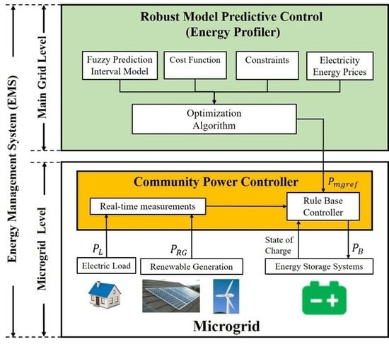
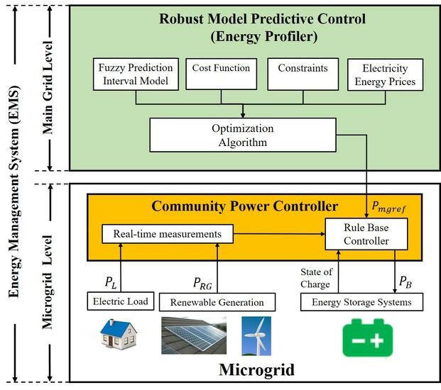
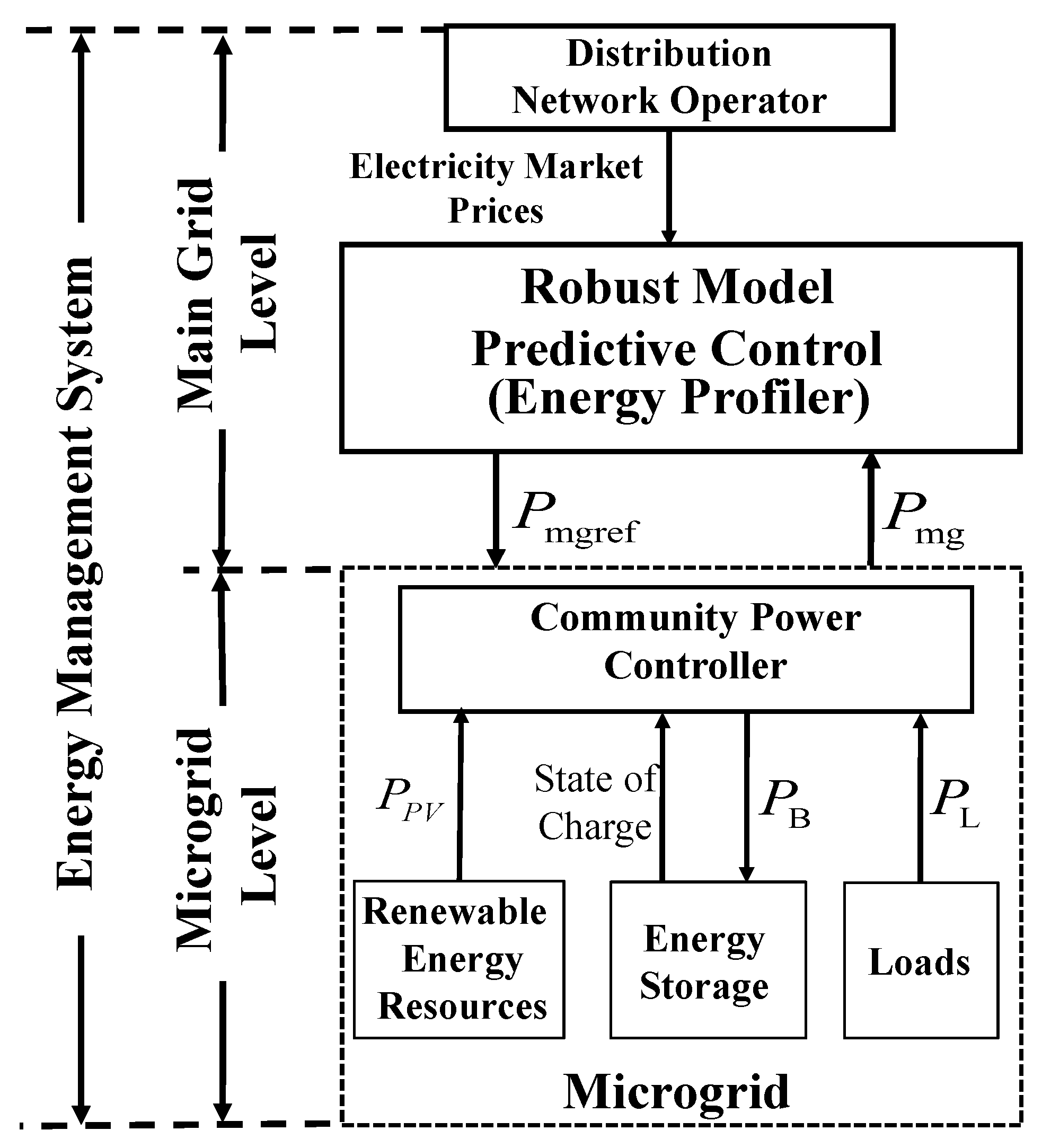
2. Problem Statement

A hierarchical EMS as in [30,31] is considered in this work. This paper presents an improvement with respect to these two, as only the lower-level controller within the hierarchy is defined in [30], while uncertainty is not tackled in [31]. The EMS in this work comprises two levels: the microgrid (energy community) level and the main grid level, as shown in Figure 1. Within this framework, the proposed microgrid is composed of domestic demand (a number of non-controllable loads), a number of renewable generation units, and an energy storage system (ESS). Several ESSs could easily be considered in the formulation by including constraints for all of them. However, a single ESS was considered here for simplicity of exposition. This configuration of microgrids is typically associated with groups of dwellings or small villages, and mainly incorporates renewable resources such as photovoltaic arrays and wind generators.
The microgrid can freely use the power from the ESS and the renewable generation, and it can purchase power from the distribution network operator (DNO) for consumption, but it cannot sell. A maximum power limit is set to reduce power peaks of the energy bought from the DNO, and no power can be sent back to it. The ESS also can consume energy in order to store it. The entire renewable generation is either consumed by the loads or stored in the ESS. In this context, the role of the DNO is to supply energy when the renewable generation and the ESS cannot provide enough power to satisfy the demand.
At the main grid level, a robust MPC controller operates to provide a realistic power reference ( P mgref ) for the microgrid, of the power to be consumed from the DNO: this is the “Energy Profiler”. At the microgrid level, the “Community Power Controller” aims to track these references in real-time.
The robust MPC implements an optimization of the predicted performance cost given by the price of the energy bought from the main grid, while considering the uncertainty associated with predictions of the renewable generation and consumer load and operational constraints. A sampling time of 30 min was considered because energy markets tend to operate with half-hourly update rates, which defines the update frequency of P mgref .
At the microgrid level, the Community Power Controller operates with a sampling time of 1 min to control the net power flowing from the main grid to the microgrid ( P mg ) in order to track the power reference ( P mgref ) sent from the Energy Profiler, while satisfying demand and guaranteeing safe ESS operation.
The following sections present the details of the Community Power Controller at the microgrid level and the robust MPC for the main grid level.

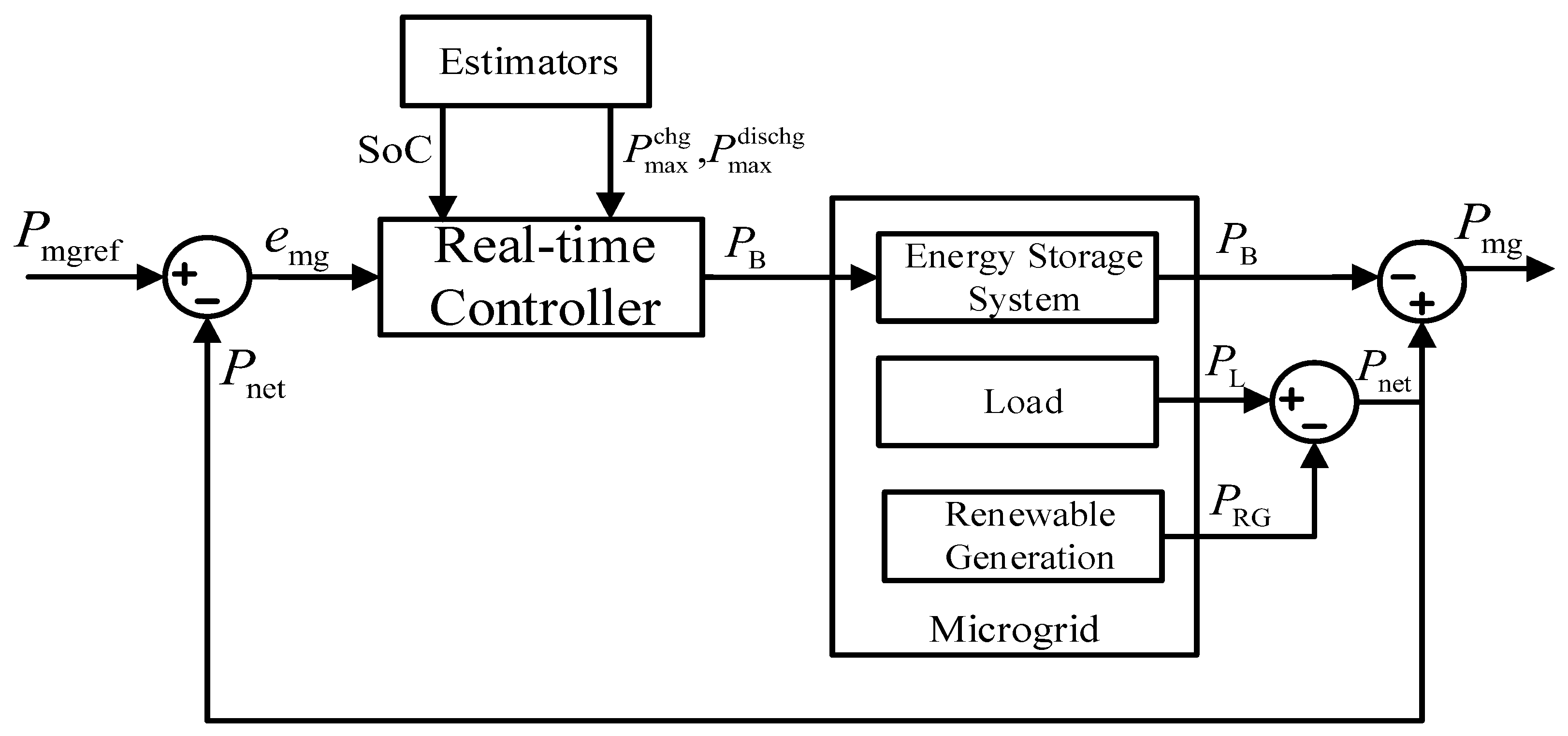
3. Community Power Controller at the Microgrid Level

The ESS is the only dispatchable DER in the proposed microgrid. Thus, the Community Power Controller can only set the charging/discharging power profile ( P B ) of the ESS (see Figure 2) in order to track P mgref as sent by the Energy Profiler. P B > 0 indicates the ESS is discharging (generation) and P B < 0 indicates the ESS is charging (load). The ESS consists of a power converter and battery packs, however converter losses are not considered in this study.
The active power of the aggregated microgrid consumption ( P L ) and aggregated renewable generation ( P RG ) are measured at the point of common coupling with a sampling rate of 1 min to calculate the net power ( P net ) of the microgrid (given by P net = P L P RG ). The error between the microgrid power target and the net power is given by:
e mg ( k ) = P mgref ( k ) P net ( k ) .
Therefore, e mg is the required power from the ESS ( P B ) so that the instantaneous microgrid power P mg tracks the target P mgref provided by the robust MPC in the Energy Profiler. Based on this, the microgrid-level controller sets the power of the ESS as P B = e mg as long as certain constraints are satisfied, as now described.
For safe operation of the ESS, the maximum available power for charging ( P max chg ) and discharging ( P max dischg ) is calculated as in [32,33]. These power values are obtained to prevent battery damage by over/under charge (state of charge, SoC) or voltage, or by exceeding the rated current or power limit. The ESS power P B cannot exceed these values. Likewise, SoC min = 0.2 and SoC max = 0.8 are the minimum and maximum values allowed for the SoC. These were set to increase the lifespan of the batteries, because capacity fade is typically accelerated by operating profiles with high average SoC and deep discharge levels [34]. To ensure operation within these limits, the SoC value is estimated based on an unscented Kalman filter [35], with outer feedback correction loops as presented in [36]. This is because Bayesian estimation algorithms have been demonstrated to be a well-suited estimation tool for nonlinear problems such as SoC estimation, and they have several advantages including real-time implementation and use of empirical models that better deal with limited and noisy data compared to methods such as ampere-hour counting, internal impedance measurement, and open circuit voltage measurement [37,38].
If the constraints defined above are violated, P B is set as close to e mg as possible to satisfy these constraints. Thus, the microgrid-level controller output P B obeys the following rules:
R 1 : i f e mg ( k ) 0 a n d S o C ( k ) S o C max t h e n P B ( k ) = 0 ; R 2 : i f e mg ( k ) 0 a n d S o C ( k ) < S o C max t h e n P B ( k ) = min ( e mg ( k ) , P max chg ( k ) ) ; R 3 : i f e mg ( k ) < 0 a n d S o C ( k ) S o C min t h e n P B ( k ) = min ( e mg ( k ) , P max dischg ( k ) ) ; R 4 : i f e mg ( k ) < 0 a n d S o C ( k ) < S o C min t h e n P B ( k ) = min ( P RG ( k ) , P max chg ( k ) ) .
The instantaneous microgrid power ( P mg ) is given by:
P mg ( k ) = P net ( k ) P B ( k ) ,
and this tracks P mgref as long as the resulting values of P B and SoC do not violate constraints.

4. Robust Model Predictive Control

The role of the higher-level controller is to calculate the reference power ( P mgref ) so that it minimizes the energy cost for the community, but also ensures that it can be tracked reasonably well by the Community Power Controller based on the available resources ( P B and P RG ) and load ( P L ) .
The proposed EMS is based on robust MPC, and thus it requires models to predict the expected value and variability of the demand, as well as the energy available from the renewable resources over a prediction horizon. Clearly, the performance of the robust EMS depends on the quality of these models. In this work, fuzzy prediction interval models are used, as presented next.

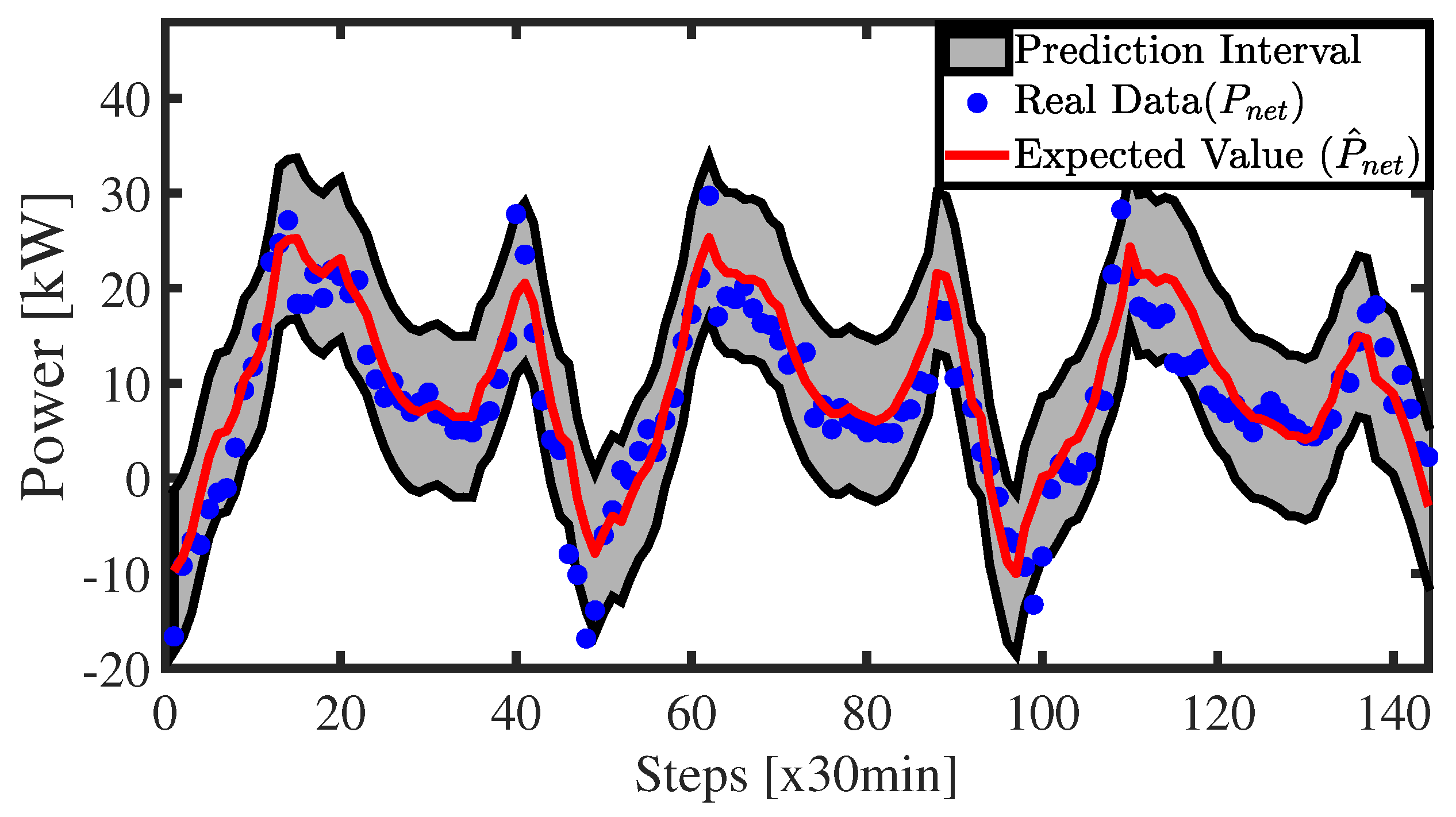
4.1. Fuzzy Prediction Interval Model

Fuzzy prediction interval models are used to predict the expected values and the uncertainty of the net power of the microgrid ( P net ). These predictions are used in the main grid-level robust MPC, with a sampling time of 30 min. Since the original data has a 1 min resolution, P net ( k ) represents the average of the measurements (made once per minute) for the 30 min following time instant k.
The fuzzy prediction interval model proposed in [39] is adopted in this work. The fuzzy model for obtaining the predicted expected value of P net is given by
P ^ net ( k ) = r = 1 R β r ( Z ( k ) ) P ^ net r ( k ) = r = 1 R β R ( Z ( k ) ) [ 1 Z ( k ) ] θ r = Ψ T Θ ,
where Z ( k ) = [ P net ( k 1 ) , , P net ( k N y ) ] , the number of rules is R, β r is the activation degree, θ r is the coefficient vector of the consequences, and P ^ net r ( k ) = [ 1 Z ( k ) ] θ r is the local output at time k of rule r, with r = 1 , , R . Ψ T = [ ψ 1 T , , ψ R T ] is the fuzzy regression matrix, and Θ T = [ θ 1 T , , θ R T ] is the coefficient matrix for all rules. The maximum regressor order corresponds to one day before ( N y = 48 ) , and some of these input variables can be discarded using a sensitivity analysis [40]. The Gustafson–Kessel clustering algorithm is used to find R and the parameters of β r ( · ) . Parameters Θ are estimated by the least-squares method [41].
The predictions for j steps ahead made at time k are:
P ^ net ( k + j ) = r = 1 R β r ( Z ( k + j ) ) P ^ net r ( k + j ) ,
where Z ( k + j ) = [ P net ( k + j 1 ) , , P net ( k + j N y ) ] , j = 1 , , N .
Fuzzy prediction interval models provide the lower ( P ^ ̲ net ( k + j ) ) and upper ( P ^ ¯ net ( k + j ) ) bounds predicted at time k such that the real values of P net ( k + j ) satisfy P ^ ̲ net ( k + j ) P net ( k + j ) P ^ ¯ net ( k + j ) , with a certain coverage probability p, for j = 1 , , N where N is the prediction horizon. It is proposed in [39] that the lower and upper bounds ( P ^ ̲ net ) and ( P ^ ¯ net ) are estimated by
P ^ ¯ net ( k + j ) = P ^ net ( k + j ) + α k + j I TS ( k + j ) ,
P ^ ̲ net ( k + j ) = P ^ net ( k + j ) α k + j I TS ( k + j ) ,
where I TS ( k + j ) = r = 1 R β r ( Z * ( k + j ) ) I r TS ( k + j ) , with I r TS ( k + j ) = σ ^ r ( 1 + ψ r * T ( ψ r ψ r T ) 1 ψ r * ) 1 / 2 , is the component associated with the covariance of the error between the observed data and the local model outputs. The current input ψ r * T is associated to a new datum Z * ( k + j ) . Additionally, α k + j are scaling parameters that are tuned using experimental data so that the interval defined by [ P ^ ̲ net ( k + j ) , P ^ ¯ net ( k + j ) ] contains the actual values of P net ( k + j ) with a given coverage probability. The next section presents deterministic and robust MPC formulations using fuzzy prediction interval modeling. The deterministic MPC is presented to illustrate the basics of the formulation, and it will be used as a basis for comparison. Focus is later given to the robust MPC, which is the main contribution of this work.

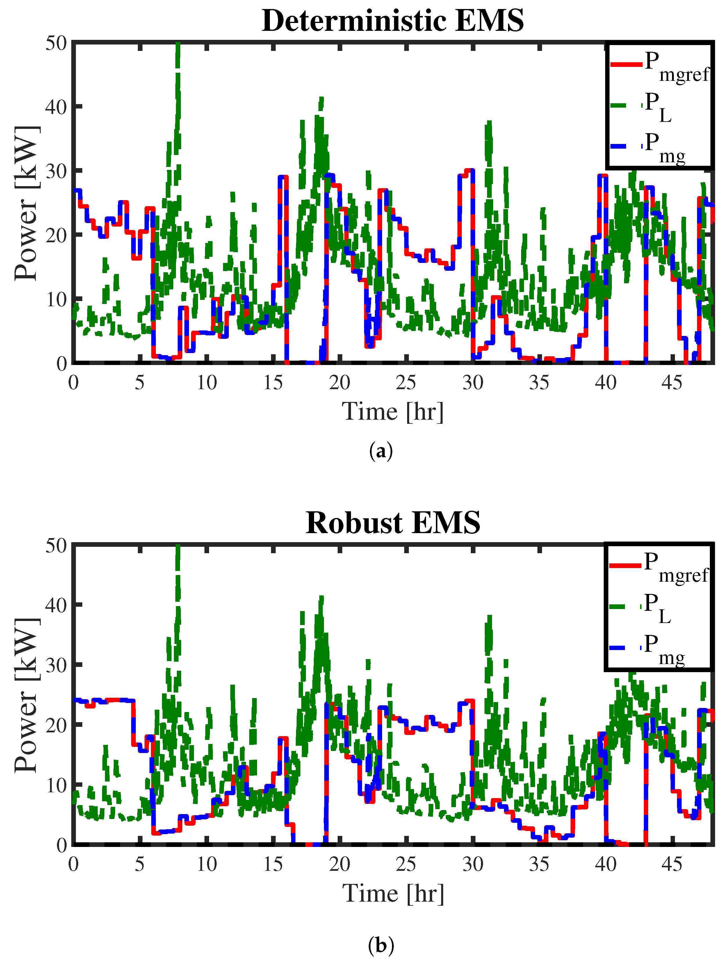
4.2. Deterministic EMS

The role of the MPC scheme at the main-grid level is to minimize the cost of the power delivered to the microgrid from the main grid. This controller uses a model of the microgrid dynamics to find its predicted behavior, which assumes that there are no losses, nor congestion or voltage regulation issues for the power transfer from the DNO to the microgrid and between elements within the microgrid. The sampling time of the model and the controller is T s = 30 min. The prediction horizon of the controller is N = 48 ; the power references one day ahead (48 steps with T s = 30 min) are found to optimize the predicted behavior for a one-day ahead operation. More precisely, at each discrete time k, an optimization problem uses this model to find the optimal sequence of P mgref ( k + j ) , j = 0 , , N 1 that minimizes the energy consumption during the prediction horizon N.
The system dynamic is given by the evolution of the energy in the ESS ( E B ) . These dynamics must be included in the MPC optimization, and are described by a simplified linear model:
E B ( k + j + 1 ) = E B ( k + j ) T s P B ( k + j ) .
The prediction of future states requires an estimation of the current state, obtained from the unscented Kalman filter at the microgrid level, which sends this information to the upper layer.
The power balance at the microgrid level must also be imposed in the MPC optimization. This constraint is invoked as
P mgref ( k + j ) = P ^ net ( k + j ) P B ( k + j ) .
Here, the net power of the microgrid is given by its expected values P ^ net ( k + j ) , which are obtained by the fuzzy prediction model defined in (5). Other constraints that must be considered in the optimization include the minimum and maximum limits of battery capacity:
E min = 0.2 C n E B ( k + j ) E max = 0.8 C n ,
where C n is the nominal capacity, and the limits for charging and discharging of the ESS are
P max dischg ( k + j ) P B ( k + j ) P max chg ( k + j ) ,
where the bounds are approximated linearly, such that P max dischg ( k + j ) = α d P B max S o C ( k + j ) and P max chg ( k + j ) = α c P B max ( 1 S o C ( k + j ) ) . Here, P B max is the maximum instantaneous power given by the manufacturer, and α d and α c are tuned parameters which avoid violation of the under/over SoC limits, respectively. The last constraints to be used are the minimum and maximum grid powers:
P mg min P mgref ( k + j ) P mg max .
Since the EMS aims to maximize self-consumption (i.e., minimize energy exported to the main grid) and to minimize the power drawn from the main grid during peak periods, P mg min = 0 was chosen, and P mg max can be chosen arbitrarily in order to reduce power peaks that are purchased from the main grid.
With these considerations, and because the EMS also aims to minimize costs, the optimal control problem to be solved at time k is given by:
min { P mgref ( k + j ) } j = 0 , , N 1 j = 0 N 1 C ( k + j ) P mgref ( k + j ) T s subject to ( 8 ) ( 12 ) all for j = 0 , , N 1 ,
where C ( k + j ) is the energy price which is a known parameter for the EMS and is based on a Time of Use tariff scheme; the price of the unit of energy depends on the hour within the day. This is a linear program. In this paper, we solved the problem using a Matlab implementation of an interior-point algorithm for linear programs. Finally, only the first element of the sequence { P mgref ( k + j ) } j = 0 , , N 1 (namely, P mgref ( k ) ) is actually sent as a reference to the microgrid, and the procedure is repeated at time k + 1 (i.e., 30 min ahead).

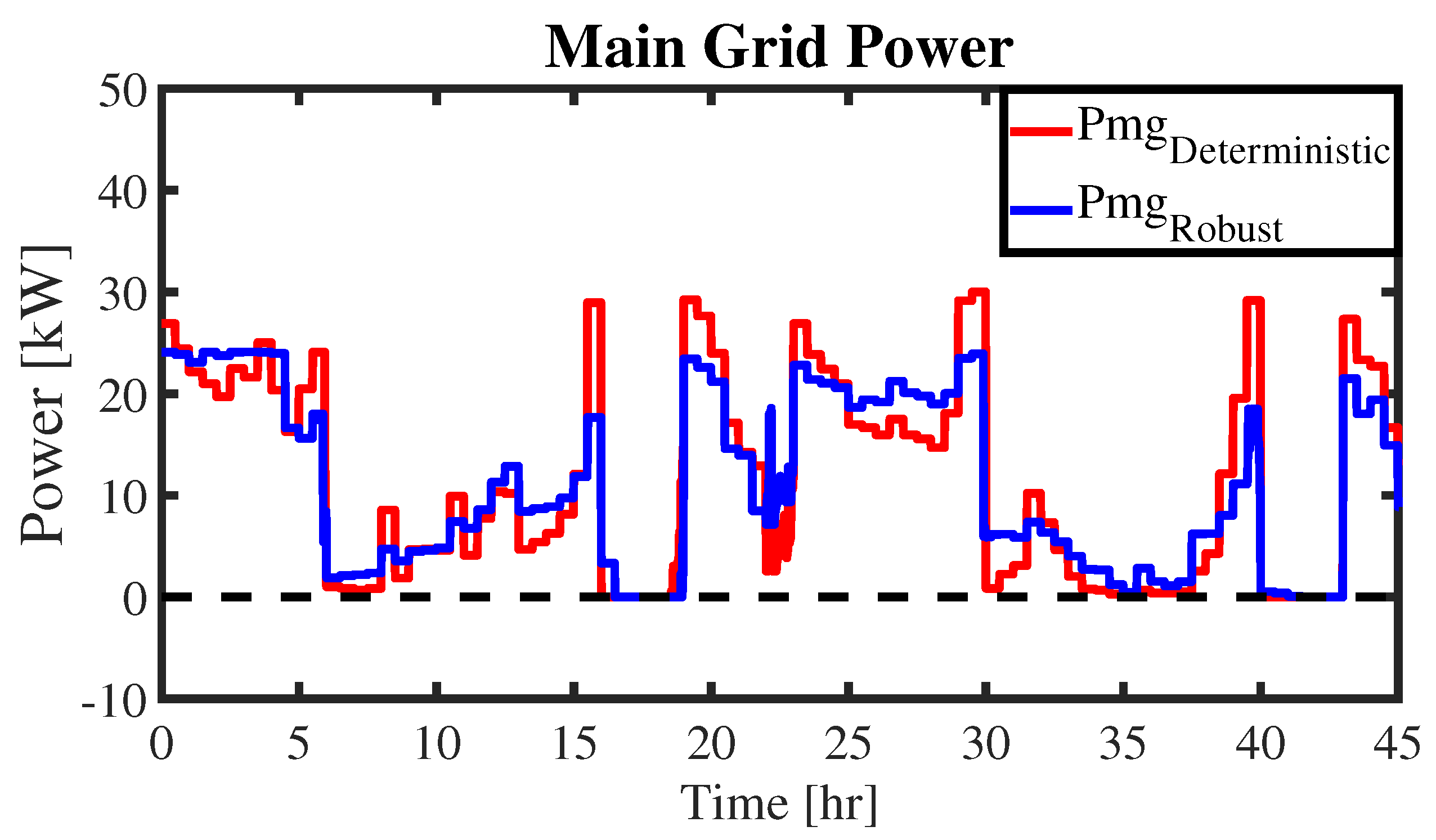
4.3. Robust EMS with Explicit Uncertainty Compensation

The formulation of Section 4.2 ignores the uncertainty of the predictions of P net . While the closed-loop nature of the controller provides some robustness to uncertainty, its explicit inclusion in the formulation may bring further benefits in performance, as discussed in [42], and will be seen in Section 5. This section deals with uncertainty handling in the controller formulation.
Fuzzy prediction interval models are used to model the uncertainty of P net predictions. The real values P net ( k + j ) satisfy P net ( k + j ) = P ^ net ( k + j ) + Δ P net ( k + j ) , where P ^ net ( k + j ) is the expected value of the prediction and Δ P net ( k + j ) is the deviation of the actual value from the prediction. This deviation is uncertain, but satisfies
Δ P net ( k + j ) [ Δ P ^ net min ( k + j ) , Δ P ^ net max ( k + j ) ] ,
where
Δ P ^ net max ( k + j ) = P ^ ¯ net ( k + j ) P ^ net ( k + j ) Δ P ^ net min ( k + j ) = P ^ ̲ net ( k + j ) P ^ net ( k + j ) ,
for j = 1 , , N 1 . These intervals are designed to have a minimum interval width and guarantee that the future real values fall within the interval with a certain coverage probability.
The solution for deterministic optimal control problems such as deterministic MPC is a sequence of fixed control actions. However, this is conservative when there are uncertain components, as this ignores the fact that there will be a correction of the disturbances by the closed-loop operation of the controller. Instead, finding a sequence of control actions or decision variables that depend on the predicted states or that can be corrected with the predicted values of uncertain variables allows the optimization to find improved solutions. It is shown in [43,44] that a computationally efficient alternative to acknowledge these corrections in the optimization is to explicitly compensate the uncertain terms with linear gains L ( k + j ) . The robust MPC formulation proposed here follows this idea, but was adapted to satisfy the power balance constraint (9). As a result, the compensation is performed either by the ESS or the main grid consumption.
The following control laws for the predicted inputs of the optimization at time k, P B and P mgref , which are coupled by (9), are proposed:
P B ( k + j ) = P ^ B ( k + j ) + L ( k + j ) Δ P ^ net ( k + j ) ,
P mgref ( k + j ) = P ^ mgref ( k + j ) + ( 1 L ( k + j ) ) Δ P ^ net ( k + j ) ,
where P ^ mgref ( k + j ) , P ^ B ( k + j ) and L ( k + j ) are the optimization variables for j = 0 , , N 1 . This can be interpreted as follows: if P net ( k + j ) = P ^ net ( k + j ) (thus Δ P ^ net ( k + j ) = 0 ), then P B ( k + j ) = P ^ B ( k + j ) . Otherwise, the predicted input to be applied to the system is compensated by L ( k + j ) Δ P ^ net ( k + j ) . Note that the compensation P mgref ( k + j ) is given by ( 1 L ( k + j ) ) Δ P ^ net ( k + j ) , so that the balance equation for the expected values
P ^ mgref ( k + j ) = P ^ net ( k + j ) P ^ B ( k + j )
is enough to satisfy the full balance for the real values (9). The following constraint is used on L ( k + j ) :
0 L ( k + j ) 1 ,
which indicates that the deviation of the real value from the prediction is compensated by P B ( k + j ) and P mgref ( k + j ) in a proportion defined by L ( k + j ) .
The predicted control laws of (16) and (17) depend on the uncertain values Δ P ^ net ( k + j ) , and so will the predictions of E B . However, the optimization problem as posed in (13) (a linear program) cannot be solved with uncertain values. A worst-case approach is taken, where Δ P ^ net ( k + j ) are assigned to take the worst possible values according to some criterion. Consider (12), which imposes the limits for P mgref and in the current setting is equivalent to
P ^ mgref ( k + j ) + ( 1 L ( k + j ) ) Δ P ^ net ( k + j ) P mg max , P ^ mgref ( k + j ) ( 1 L ( k + j ) ) Δ P ^ net ( k + j ) P mg min .
These inequalities depend on Δ P ^ net ( k + j ) , which is uncertain, so it is not known what value it will take. Therefore, these are enforced by taking a worst-case approach, as is common in robust MPC. They are implemented by setting Δ P ^ net ( k + j ) to take the values that reduce freedom the most for P ^ mgref ( k + j ) in each of the inequalities: Δ P ^ net max ( k + j ) and P ^ net min ( k + j ) , respectively. Thus, the constraints above are enforced in the optimization as
P ^ mgref ( k + j ) + ( 1 L ( k + j ) ) Δ P ^ net max ( k + j ) P mg max , P ^ mgref ( k + j ) + ( 1 L ( k + j ) ) Δ P ^ net min ( k + j ) P mg min .
Note that these constraints are linear because Δ P ^ net max ( k + j ) , Δ P ^ net min ( k + j ) are known for the optimization, and only P ^ mgref ( k + j ) and L ( k + j ) are optimization variables. For all constraints associated with the ESS, the worst case is considered to be that where P net ( k + j ) is the largest; that is, Δ P net ( k + j ) : = Δ P ^ net max ( k + j ) . This is the case with the most deficit of renewables with respect to demand, which is the instant where the ESS is needed the most to provide flexibility and reduce the energy bought from the grid. Therefore, constraints (8), (10), and (11) are reformulated as:
T s i = 0 j P ^ B ( k + i ) T s i = 0 j L ( k + i ) Δ P ^ net max ( k + i ) E max E B ( k ) ,
T s i = 0 j P ^ B ( k + i ) + T s i = 0 j L ( k + i ) Δ P ^ net max ( k + i ) E min + E B ( k ) ,
P ^ B ( k + j ) + L ( k + j ) Δ P ^ net max ( k + j ) P max dischg ( k + j ) , P ^ B ( k + j ) + L ( k + j ) Δ P ^ net max ( k + j ) P max chg ( k + j ) .
With all these considerations, the optimization problem to be solved at each time k is
min x j = 0 N 1 C ( k + j ) P ^ mgref ( k + j ) T s subject to ( 18 ) ( 23 ) all for j = 0 , , N 1 ,
where x = { P ^ mgref ( k + j ) , P ^ B ( k + j ) , L ( k + j ) } j = 0 , , N 1 .
This is also a linear program, and is solved with the same Matlab solver as for (13). Finally, P mgref ( k ) is sent as a reference to the microgrid, and the procedure is repeated at time k + 1 .
Using this robust MPC guarantees the satisfaction of constraints for the worst cases incorporated in the optimization. For instance, it ensures that the power reference sent does not instruct the lower level to sell energy to the grid nor that the power bought is greater than the upper limit. On the other hand, using worst-case constraints may introduce conservativeness to the solutions, which may be reflected as economic costs, because worst cases may not occur.

5. Case Study

The performance of the hierarchical EMS based on robust MPC was tested by the simulation of a community connected to the main grid, made up of 30 dwellings with a 50% level of photovoltaic power penetration (i.e., 15 dwellings have a photovoltaic array) and an ESS made of lead-acid batteries with a 135-kWh capacity.
Data for winter from a town in the UK was used [45]. For this scenario, a three-level Time of Use tariff (similar to [46]) was considered for buying energy from the grid for each day of the simulation. The prices are shown in Table 1.

5.1. Fuzzy Prediction Interval for Net Power of the Microgrid

Load and photovoltaic power data available for a town in the UK were used to develop the fuzzy prediction interval model described in Section 4.1 for the net power given by P net = P L P RG . The data cover a period of 90 days corresponding to the winter season, and this was divided into training, validation, and test data sets. The maximum value of P net was 67.57 kW and the minimum value was −45.09 kW, and a sampling time of 30 min was used.
The fuzzy model and regressors obtained during the identification for the predictor of P net ( k ) were:
P ^ net ( k ) = f fuzzy ( P net ( k i 1 ) , , P net ( k i n ) ) ,
where { i 1 , , i n } = { 1 , 2 , 8 , 25 , 26 , 32 , 38 , 42 , 43 , 44 , 46 , 48 } and the optimal structure of the model has four rules. Note that exogenous variables were not included in the model.
The prediction interval coverage probability (PICP), which quantifies the proportion of measured values that fall within the predicted interval, and the prediction interval normalized average width (PINAW), which quantifies the width of the interval, were used as indexes to evaluate the quality of the interval for h-step-ahead predictions:
PICP ( h ) = 1 T k = 1 T δ k + h ,
PINAW ( h ) = 1 T R k = 1 T P ^ ¯ net ( k + h ) P ^ ̲ net ( k + h ) ,
for h = 1 , , N , where P net ( k ) is the real value of P net , R is the distance between the maximum and minimum values of P net ( k ) in the data set, and δ k + h = 1 if P net ( k + h ) [ P ^ ¯ net ( k + h ) , P ^ ̲ net ( k + h ) ] ; otherwise, δ k + h = 0 . Additionally, the root mean square error (RMSE) and the mean absolute error (MAE) were used to evaluate the accuracy of the prediction model associated with the expected value.
In this study, the prediction interval model was tuned at a PICP of 90% for all prediction instants. Table 2 shows the performance indexes associated with three different prediction horizons for the test dataset. The results indicate that the fuzzy prediction interval was effectively tuned to a PICP of 90%, and that the interval width (PINAW) increased with the prediction horizon. Figure 3 shows the one-day-ahead prediction intervals for three days of the test dataset. The red line is the one-ahead prediction ( P ^ net ) of the net power of the microgrid ( P net ) , the blue points are the actual data ( P net ) used to evaluate the performance of the fuzzy prediction interval model, and the grey box is the prediction interval which is characterized by the lower ( P ^ ̲ net ) and upper ( P ^ ¯ net ) bounds.
The expected value ( P ^ net ) and lower ( P ^ ̲ net ) and upper ( P ^ ¯ net ) bound predictions provided by the prediction interval were used in the deterministic and robust EMSs, as explained in Section 4.2 and Section 4.3.

5.2. Hierarchical EMS Results

The performance of the EMS based on robust MPC with fuzzy interval models (Section 4.3) is analyzed in this section. For this purpose, it was compared with the deterministic EMS presented in Section 4.2. Simulation results for this comparison are presented in the following.
Figure 4 shows the responses obtained with the hierarchical EMSs (deterministic and robust) for operation over two days. Results were consistent with the daily distribution of the energy prices. Since energy from the main grid was most expensive in the 16:00–19:00 h time block, the EMS controlled this power to be close to zero. The opposite behavior occurred during morning and late night hours (0:00–06:00 and 23:00–24:00) when the energy price was considerably cheaper. It can also be seen that in both deterministic and robust approaches the power reference ( P mgref ), as sent by the higher-level MPC controller (in red), could be tracked reasonably well by the lower-level controller ( P mg , in blue). Tracking errors occurred when the maximum available battery power for charging or discharging was less than the ESS power required by the microgrid (see the rules in Section 3). Additionally, Figure 4 shows that the robust EMS found a flatter P mgref than the deterministic EMS, which is good for the distribution network operator because it minimizes the grid power profile fluctuations. Several metrics justify and quantify the flattening, as will be discussed below.
Table 3 shows the energy costs, the RMSE of the tracking error of the power reference ( P mgref ) , the equivalent full cycles (EFC), and the loss of power supply probability (LPSP) for one week of simulation using the deterministic and robust EMSs (see Appendix A for definition of EFC and LPSP). It can be seen that the robust EMS reached a better operation cost than the deterministic EMS. Additionally, the lower RMSE with the robust EMS means that there was a better tracking of the power reference ( P mgref ) sent by the higher level to the microgrid (see Figure 4). The lower EFC of the robust EMS means that fewer cycles were used by the ESS which directly improved the state-of-health and lifetime of the ESS. As battery aging (measured by the state-of-health) is a function of the elapsed time from the manufacture date, as well as the usage by consecutive charge and discharge actions, a lower EFC improves the battery life time. Finally, the LPSP, which is the fraction of time where the microgrid cannot fulfill the load requirements using the reference power ( P mgref ) defined by the higher level and the available resources of the microgrid (renewable generation and ESS), was 3.780% for the deterministic EMS and 2.927% for the robust EMS. This was because the robust approach compensated for the uncertainty of generation and demand and could avoid the scenarios measured by the LPSP.
Table 4 shows the energy bought by the community from the main grid during the time periods associated with different tariff prices. C1 is the time with the cheapest price and C3 is the time with the highest price. As discussed above, the operation of both hierarchical EMSs was consistent with these price bands: more energy was bought at C1 and C2, less energy was bought at C3. Note that the robust EMS bought more at C1 than the deterministic EMS. However, it spent less in C2 and considerably less than the deterministic EMS at C3. It is apparent then that the robust EMS managed to obtain savings with respect to the deterministic EMS by being better at planning against worst cases; namely, it avoided buying energy when it was most expensive.
Finally, for further evaluation of the EMSs, several indexes of operation are presented in Table 5. These are the load factor (LF), the load loss factor (LLF), positive power peak ( P + ) , negative power peak ( P ) , the maximum power derivative (MPD), and the average power derivative (APD). See Appendix A for detailed definitions, but the interpretations of these are presented next.
The LF describes the flatness of the power response: values close to 1 are associated with flat responses while values close to 0 indicate the presence of large peaks. The LLF quantifies the losses incurred as a result of peak power: values close to 1 describe flat responses with small losses, while values close to 0 indicate large losses due to large peaks [7]. The MPD is the maximum value of the rate of change between two consecutive points of the main grid power in its absolute value [10,47]. The APD is the average of the absolute value of the rate of change of the main grid power.
The LF was greater for the robust EMS than for the deterministic case (LF = 0.4459 and LF = 0.3869, respectively). This clearly indicates that the response for the robust EMS was flatter (which is also consistent with the results of RMSE and EFC reported above). Similarly, LLF = 0.288 for the robust EMS, and LF = 0.2452 for the deterministic EMS. Therefore, the hierarchical EMSs resulted in a reduction of the peak power and a reduction of losses due to peak power.
The positive power peak ( P + ) and negative power peak ( P ) for the hierarchical EMS were limited by constraints as explained in Section 4. The limits were P mg min = 0 kW, which guarantees that no energy was exported to the main grid, and P mg max = 30 kW. The robust EMS works in a more conservative manner for the upper limit. It attempts to avoid sub-optimal operation due to worst-case scenarios: thus, it allows smaller peaks ( P + = 25.9 ) kW than the deterministic EMS ( 30 kW ) (see also Figure 5).
The last two metrics were also improved using the proposed robust-MPC-based EMS: the MPD and APD were reduced compared with the deterministic EMS. Finally, a lower APD corresponds to a flatter main grid power, which is consistent with previously analyzed indicators.
Overall, it can be seen that the deterministic and robust hierarchical EMSs provide mechanisms for efficient energy management. However, the robust EMS provided improvements over the deterministic EMS, which can be explained because the uncertainty management in the robust EMS helps the system to be prepared for errors in the predictions that might yield sub-optimal decisions.

6. Conclusions

In this paper, a two-level hierarchical EMS based on robust MPC was presented for the operation of energy communities (microgrids), considering the uncertainty of the renewable energy resources and electrical load consumption. The robust MPC has a special structure which enables compensation of the uncertain predictions by the battery within the microgrid or consumption from the main grid.
While the deterministic EMS could effectively operate the microgrid, the robust EMS consistently performed better over several indicators of performance considered in the work. Most importantly: improved operational cost, flatter response of the power drawn from the main grid, and a greater capacity to satisfy demand from the microgrid. This is because robust MPC handles uncertainty and prepares better for unexpected changes in the microgrid generation or loads.
Future work will incorporate real-time prices in the formulation to reflect the price on the wholesale market. A market scheme that allows the selling of excess energy from the microgrid to the main grid will also be considered. Additionally, the benefits of the proposed hierarchical EMS based on robust MPC will be explored for energy communities such as factories, schools, commercial parks, among others; other communities using different types of loads; distributed generations, such as biomass-based generation; or energy storage technologies, such as hydrogen or flywheels. Finally, the incorporation of demand-side management (DSM) strategies into the robust MPC formulation could be studied to determine an optimal demand schedule, helping to generate desired changes in the load profile.

Author Contributions

Conceptualization, L.G.M., M.S., S.P., and D.S.; methodology, L.G.M., D.M.-C., and D.S.; software, L.G.M. and D.K.; validation, L.G.M., D.M.-C., and D.S.; formal analysis, L.G.M., D.M.-C., and A.N.; Writing—Original draft preparation, L.G.M.; Writing—review and editing, L.G.M., M.S., D.M.-C., D.K., S.P., D.S., and A.N.

Funding

This research was funded by the Instituto Sistemas Complejos de Ingeniería (ISCI) (CONICYT PIA/BASAL AFB180003), the Solar Energy Research Center SERC-Chile (CONICYT/FONDAP/Project under Grant 15110019), FONDECYT Chile Grant Nr. 1170683 “Robust Distributed Predictive Control Strategies for the Coordination of Hybrid AC and DC Microgrids” and CONICYT-FONDECYT Postdoctorado-3170040. Luis Gabriel Marín has also been supported by a Ph.D. scholarship from COLCIENCIAS-Colombia and by a scholarship from CONICYT-PCHA/Doctorado Nacional para extranjeros/2014-63140093.

Conflicts of Interest

The authors declare no conflicts of interest.

Abbreviations

The following abbreviations are used in this manuscript:
EMSEnergy management system
MPCModel predictive control
DNODistribution network operator
DERDistributed energy resource
DGDistributed generation
DNDistribution network
ESSEnergy storage system
SoCState of charge
PICPPrediction interval coverage probability
PINAWPrediction interval normalized average width
RMSERoot mean square error
MAEMean absolute error
EFCEquivalent full cycles
LPSPLoss of power supply probability
LFLoad Factor
LLFLoad loss factor
MPDMaximum power derivative
APDAverage power derivative

Appendix A. Performance Indices for the Power Profile of the Main Grid

Several indexes that evaluate the quality of the power profiles sent from the main grid to the micro-grid were used to compare the results obtained with the different control strategies. These indices are described in the following.
RMSE is the root mean square error:
RMSE = k = 1 T ( P mgref ( k ) P mg ( k ) ) 2 T ,
which represents the capability of the microgrid to follow the power reference ( P mgref ) sent by the higher level in the hierarchical EMS.
The equivalent full cycles (EFC) is the number of full discharges that an ESS performs throughout its time use [48]:
EFC = E dis ( A h ) C n ,
where E dis [ A h ] is the discharge energy during the simulation time and C n is the nominal battery capacity. The EFC is a metric associated with the life cycle of the ESS. In this approach, one cycle per day is the desired EFC ( EFC desired ).
The loss of power supply probability (LPSP) is the ratio between the energy deficiency and the total energy demands for a period of time [49]. In this approach, the energy deficiency occurs when ( P net ( k ) P mgref ( k ) ) T s > 0 , which means that the available maximum power of the ESS ( P max dischg ) cannot fulfill the load, and therefore the energy deficiency is supplied from the main grid. When this happens, the microgrid cannot follow the power reference ( P mgref ) perfectly, and therefore P mg = P mgref + ED . A lower value of LPSP indicates a higher probability that the load will be satisfied. The LPSP is defined as [50]
LPSP = k = 1 T T k T ,
where T k is the number of instants when an energy deficiency occurs and T is the total simulation time. The load factor (LF) is given by
LF = Avg ( P mg ) max ( P mg ) ,
and quantifies the ratio between the average grid power ( P mg AVG ) and peak grid power ( P mg max ) during a given period. An improvement to the LF value indicates a peak load reduction.
The load loss factor (LLF) is a measure of losses incurred as a result of peak power:
LLF = Avg ( P mg 2 ) max ( P mg 2 ) .
The maximum power derivative (MPD) is the maximum value of the rate of change between two consecutive points of the main grid power in its absolute value:
MPD = max ( | Δ P mg ( k ) | ) ,
where Δ P mg ( k ) = P mg ( k ) P mg ( k 1 ) .
Finally, the average power derivative (APD) is the average of the absolute value of the rate of change of the main grid power
APD = 1 T k = 1 T | Δ P mg ( k ) | .
In this Appendix, the maximum and minimum values were taken over the whole simulation period.

References

  1. Padhi, P.P.; Pati, R.K.; Nimje, A.A. Distributed generation: Impacts and cost analysis. Int. J. Power Syst. Oper. Energy Manag. 2012, 1, 91–96. [Google Scholar]
  2. Hidalgo, R.; Abbey, C.; Joós, G. A review of active distribution networks enabling technologies. In Proceedings of the IEEE PES General Meeting, Providence, RI, USA, 25–29 July 2010; pp. 1–9. [Google Scholar] [CrossRef]
  3. Abapour, S.; Zare, K.; Mohammadi-Ivatloo, B. Dynamic planning of distributed generation units in active distribution network. IET Gener. Transm. Distrib. 2015, 9, 1455–1463. [Google Scholar] [CrossRef]
  4. Palizban, O.; Kauhaniemi, K.; Guerrero, J.M. Microgrids in active network management—Part II: System operation, power quality and protection. Renew. Sustain. Energy Rev. 2014, 36, 440–451. [Google Scholar] [CrossRef]
  5. Mirzania, P.; Andrews, D.; Ford, A.; Maidment, G. Community Energy in the UK: The End or the Beginning of a Brighter Future? In Proceedings of the 1st International Conference on Energy Research and Social Science, Sitges, Spain, 5–7 April 2017. [Google Scholar]
  6. Lefroy, J. Local Electricity Bill. Available online: https://powerforpeople.org.uk/wp-content/uploads/2019/03/Local-Electricity-Bill.pdf (accessed on 3 October 2019).
  7. Fazeli, A.; Sumner, M.; Johnson, M.C.; Christopher, E. Real-time deterministic power flow control through dispatch of distributed energy resources. IET Gener. Transm. Distrib. 2015, 9, 2724–2735. [Google Scholar] [CrossRef]
  8. Daud, A.K.; Ismail, M.S. Design of isolated hybrid systems minimizing costs and pollutant emissions. Renew. Energy 2012, 44, 215–224. [Google Scholar] [CrossRef]
  9. Hosseinzadeh, M.; Salmasi, F.R. Power management of an isolated hybrid AC/DC microgrid with fuzzy control of battery banks. IET Renew. Power Gener. 2015, 9, 484–493. [Google Scholar] [CrossRef]
  10. Arcos-Aviles, D.; Pascual, J.; Marroyo, L.; Sanchis, P.; Guinjoan, F. Fuzzy Logic-Based Energy Management System Design for Residential Grid-Connected Microgrids. IEEE Trans. Smart Grid 2018, 9, 530–543. [Google Scholar] [CrossRef]
  11. Davies, R.; Sumner, M.; Christopher, E. Energy storage control for a small community microgrid. In Proceedings of the 7th IET International Conference on Power Electronics, Machines and Drives, Manchester, UK, 8–10 April 2014; pp. 1–6. [Google Scholar] [CrossRef]
  12. Silvente, J.; Kopanos, G.M.; Pistikopoulos, E.N.; Espuña, A. A rolling horizon optimization framework for the simultaneous energy supply and demand planning in microgrids. Appl. Energy 2015, 155, 485–501. [Google Scholar] [CrossRef]
  13. Palma-Behnke, R.; Benavides, C.; Lanas, F.; Severino, B.; Reyes, L.; Llanos, J.; Sáez, D. A Microgrid Energy Management System Based on the Rolling Horizon Strategy. IEEE Trans. Smart Grid 2013, 4, 996–1006. [Google Scholar] [CrossRef]
  14. Parisio, A.; Rikos, E.; Glielmo, L. A Model Predictive Control Approach to Microgrid Operation Optimization. IEEE Trans. Control Syst. Technol. 2014, 22, 1813–1827. [Google Scholar] [CrossRef]
  15. Olivares, D.E.; Cañizares, C.A.; Kazerani, M. A Centralized Energy Management System for Isolated Microgrids. IEEE Trans. Smart Grid 2014, 5, 1864–1875. [Google Scholar] [CrossRef]
  16. Ji, Z.; Huang, X.; Xu, C.; Sun, H. Accelerated Model Predictive Control for Electric Vehicle Integrated Microgrid Energy Management: A Hybrid Robust and Stochastic Approach. Energies 2016, 9, 973. [Google Scholar] [CrossRef]
  17. Li, Z.; Zang, C.; Zeng, P.; Yu, H. Combined Two-Stage Stochastic Programming and Receding Horizon Control Strategy for Microgrid Energy Management Considering Uncertainty. Energies 2016, 9, 499. [Google Scholar] [CrossRef]
  18. Brandstetter, M.; Schirrer, A.; Miletić, M.; Henein, S.; Kozek, M.; Kupzog, F. Hierarchical Predictive Load Control in Smart Grids. IEEE Trans. Smart Grid 2017, 8, 190–199. [Google Scholar] [CrossRef]
  19. Shayeghi, H.; Shahryari, E.; Moradzadeh, M.; Siano, P. A Survey on Microgrid Energy Management Considering Flexible Energy Sources. Energies 2019, 12, 2156. [Google Scholar] [CrossRef]
  20. Lara, J.D.; Olivares, D.E.; Cañizares, C.A. Robust Energy Management of Isolated Microgrids. IEEE Syst. J. 2018, 1–12. [Google Scholar] [CrossRef]
  21. Wu, W.; Chen, J.; Zhang, B.; Sun, H. A Robust Wind Power Optimization Method for Look-Ahead Power Dispatch. IEEE Trans. Sustain. Energy 2014, 5, 507–515. [Google Scholar] [CrossRef]
  22. Khodaei, A. Provisional Microgrids. IEEE Trans. Smart Grid 2015, 6, 1107–1115. [Google Scholar] [CrossRef]
  23. Yi, J.; Lyons, P.F.; Davison, P.J.; Wang, P.; Taylor, P.C. Robust Scheduling Scheme for Energy Storage to Facilitate High Penetration of Renewables. IEEE Trans. Sustain. Energy 2016, 7, 797–807. [Google Scholar] [CrossRef]
  24. Malysz, P.; Sirouspour, S.; Emadi, A. An Optimal Energy Storage Control Strategy for Grid-connected Microgrids. IEEE Trans. Smart Grid 2014, 5, 1785–1796. [Google Scholar] [CrossRef]
  25. Valencia, F.; Collado, J.; Sáez, D.; Marín, L.G. Robust Energy Management System for a Microgrid Based on a Fuzzy Prediction Interval Model. IEEE Trans. Smart Grid 2016, 7, 1486–1494. [Google Scholar] [CrossRef]
  26. Du, Y.; Pei, W.; Chen, N.; Ge, X.; Xiao, H. Real-time microgrid economic dispatch based on model predictive control strategy. J. Mod. Power Syst. Clean Energy 2017, 5, 787–796. [Google Scholar] [CrossRef]
  27. Zhang, Y.; Fu, L.; Zhu, W.; Bao, X.; Liu, C. Robust model predictive control for optimal energy management of island microgrids with uncertainties. Energy 2018, 164, 1229–1241. [Google Scholar] [CrossRef]
  28. Velarde, P.; Maestre, J.M.; Ocampo-Martinez, C.; Bordons, C. Application of robust model predictive control to a renewable hydrogen-based microgrid. In Proceedings of the 2016 European Control Conference (ECC), Aalborg, Denmark, 29 June–1 July 2016; pp. 1209–1214. [Google Scholar] [CrossRef]
  29. Pereira, M.; de la Peña, D.M.; Limon, D. Robust economic model predictive control of a community micro-grid. Renew. Energy 2017, 100, 3–17. [Google Scholar] [CrossRef]
  30. Fazeli, A.; Sumner, M.; Christopher, E.; Johnson, M. Power flow control for power and voltage management in future smart energy communities. In Proceedings of the 3rd Renewable Power Generation Conference, Naples, Italy, 24–25 September 2014; pp. 1–6. [Google Scholar] [CrossRef]
  31. Elkazaz, M.; Sumner, M.; Thomas, D. Real-Time Energy Management for a Small Scale PV-Battery Microgrid: Modeling, Design, and Experimental Verification. Energies 2019, 12, 2712. [Google Scholar] [CrossRef]
  32. Plett, G.L. High-performance battery-pack power estimation using a dynamic cell model. IEEE Trans. Veh. Technol. 2004, 53, 1586–1593. [Google Scholar] [CrossRef]
  33. Sun, F.; Xiong, R.; He, H.; Li, W.; Aussems, J.E. Model-based dynamic multi-parameter method for peak power estimation of lithium–ion batteries. Appl. Energy 2012, 96, 378–386. [Google Scholar] [CrossRef]
  34. Pérez, A.; Moreno, R.; Moreira, R.; Orchard, M.; Strbac, G. Effect of Battery Degradation on Multi-Service Portfolios of Energy Storage. IEEE Trans. Sustain. Energy 2016, 7, 1718–1729. [Google Scholar] [CrossRef]
  35. Der Merwe, R.V.; Wan, E.A. The square-root unscented Kalman filter for state and parameter-estimation. In Proceedings of the 2001 IEEE International Conference on Acoustics, Speech, and Signal Processing, Salt Lake City, UT, USA, 7–11 May 2001; Volume 6, pp. 3461–3464. [Google Scholar] [CrossRef]
  36. Tampier, C.; Pérez, A.; Jaramillo, F.; Quintero, V.; Orchard, M.; Silva, J. Lithium-ion battery end-of-discharge time estimation and prognosis based on Bayesian algorithms and outer feedback correction loops: A comparative analysis. In Proceedings of the Annual Conference of the Prognostics and Health Management Society, San Diego, CA, USA, 18–24 October 2015; Volume 6, pp. 182–195. [Google Scholar]
  37. Burgos, C.; Sáez, D.; Orchard, M.E.; Cárdenas, R. Fuzzy modelling for the state-of-charge estimation of lead-acid batteries. J. Power Sources 2015, 274, 355–366. [Google Scholar] [CrossRef]
  38. Pola, D.A.; Navarrete, H.F.; Orchard, M.E.; Rabié, R.S.; Cerda, M.A.; Olivares, B.E.; Silva, J.F.; Espinoza, P.A.; Pérez, A. Particle-Filtering-Based Discharge Time Prognosis for Lithium-Ion Batteries with a Statistical Characterization of Use Profiles. IEEE Trans. Reliab. 2015, 64, 710–720. [Google Scholar] [CrossRef]
  39. Sáez, D.; Ávila, F.; Olivares, D.; Cañizares, C.; Marín, L. Fuzzy Prediction Interval Models for Forecasting Renewable Resources and Loads in Microgrids. IEEE Trans. Smart Grid 2015, 6, 548–556. [Google Scholar] [CrossRef]
  40. Sáez, D.; Zuniga, R. Cluster optimization for Takagi & Sugeno fuzzy models and its application to a combined cycle power plant boiler. In Proceedings of the 2004 American Control Conference, Boston, MA, USA, 30 June–2 July 2004; Volume 2, pp. 1776–1781. [Google Scholar] [CrossRef]
  41. Babuška, R. Fuzzy Modeling for Control, 1st ed.; Kluwer Academic Publishers: Boston, MA, USA, 1998; p. 288. [Google Scholar] [CrossRef]
  42. Kouvaritakis, B.; Cannon, M. Model Predictive Control: Classical, Robust and Stochastic, 1st ed.; Springer: Berlin, Germany, 2016; p. 384. [Google Scholar] [CrossRef]
  43. Goulart, P.J.; Kerrigan, E.C.; Maciejowski, J.M. Optimization over state feedback policies for robust control with constraints. Automatica 2006, 42, 523–533. [Google Scholar] [CrossRef] [Green Version]
  44. Kouvaritakis, B.; Cannon, M.; Muñoz-Carpintero, D. Efficient prediction strategies for disturbance compensation in stochastic MPC. Int. J. Syst. Sci. 2013, 44, 1344–1353. [Google Scholar] [CrossRef]
  45. Richardson, I.; Thomson, M. One-Minute Resolution Domestic Electricity Use Data, 2008–2009. Colch. Essex UK Data Arch. 2010. [Google Scholar] [CrossRef]
  46. Green Energy UK. Tide—A New Way to Take Control; Green Energy UK: Ware, UK; Available online: https://www.greenenergyuk.com/Tide (accessed on 3 October 2019).
  47. Pascual, J.; Barricarte, J.; Sanchis, P.; Marroyo, L. Energy management strategy for a renewable-based residential microgrid with generation and demand forecasting. Appl. Energy 2015, 158, 12–25. [Google Scholar] [CrossRef]
  48. Parra, D.; Norman, S.A.; Walker, G.S.; Gillott, M. Optimum community energy storage for renewable energy and demand load management. Appl. Energy 2017, 200, 358–369. [Google Scholar] [CrossRef]
  49. Zahboune, H.; Zouggar, S.; Krajacic, G.; Varbanov, P.S.; Elhafyani, M.; Ziani, E. Optimal hybrid renewable energy design in autonomous system using Modified Electric System Cascade Analysis and Homer software. Energy Convers. Manag. 2016, 126, 909–922. [Google Scholar] [CrossRef]
  50. Bilal, B.O.; Sambou, V.; Ndiaye, P.A.; Kébé, C.M.F.; Ndongo, M. Multi-objective design of PV-wind-batteries hybrid systems by minimizing the annualized cost system and the loss of power supply probability (LPSP). In Proceedings of the 2013 IEEE International Conference on Industrial Technology (ICIT), Cape Town, South Africa, 25–28 Feburary 2013; pp. 861–868. [Google Scholar] [CrossRef]
Figure 1. Hierarchical energy management system (EMS) Structure.
Energies 12 04453 g001
Figure 2. Block diagram at the microgrid level. SoC: state of charge.
Energies 12 04453 g002
Figure 3. One-day-ahead prediction interval for P net tuned at P I C P = 90 % .
Energies 12 04453 g003
Figure 4. Performance of the proposed hierarchical EMS: (a) Deterministic approach; (b) Robust approach.
Energies 12 04453 g004
Figure 5. Main grid power profiles.
Energies 12 04453 g005
Table 1. Energy price during the day.
Hours00:00–06:0006:00–16:0016:00–19:0019:00–23:0023:00–24:00
Energy Cost5 p/kWh12 p/kWh25 p/kWh12 p/kWh5 p/kWh
Table 2. Performance indices of fuzzy prediction interval model. MAE: mean absolute error; PICP: prediction interval coverage probability; PINAW: prediction interval normalized average width; RMSE: root mean square error.
Performance IndicesPrediction Horizon
One Hour AheadSix Hours AheadOne Day Ahead
RMSE (kW)4.51365.04715.1974
MAE (kW)3.29953.73163.7530
PINAW (%)22.7327.6228.02
PICP (%)88.2289.7989.83
Table 3. Performance indices during a simulation of one-week duration. EFC: equivalent full cycles; LPSP: loss of power supply probability.
EMS StrategyCostRMSEEFCLPSP
(£)(kW)Cycles(%)
Deterministic EMS168.011.226.403.780
Robust EMS165.281.146.072.927
Table 4. Energy distribution at different prices.
EMS StrategyC1C2C3
(kWh)(kWh)(kWh)
Deterministic990.361934.33825.483
Robust994.081931.23115.321
Table 5. Quality indexes for the power profile of the main grid. APD: average power derivative; LF: load factor; LLF: load loss factor; MPD: maximum power derivative.
EMS StrategyLFLLF P + P MPDAPD
(kW)(kW)(kW/min)(kW/min)
Deterministic0.38690.245230.00029.630.1889
Robust0.44590.288025.90022.480.1318

