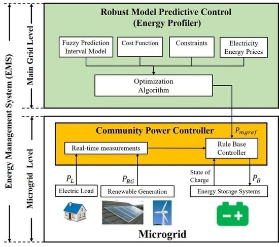
Hierarchical Energy Management System for Microgrid Operation Based on Robust Model Predictive Control
Abstract
1. Introduction
2. Problem Statement
3. Community Power Controller at the Microgrid Level
4. Robust Model Predictive Control
4.1. Fuzzy Prediction Interval Model
4.2. Deterministic EMS
4.3. Robust EMS with Explicit Uncertainty Compensation
5. Case Study
5.1. Fuzzy Prediction Interval for Net Power of the Microgrid
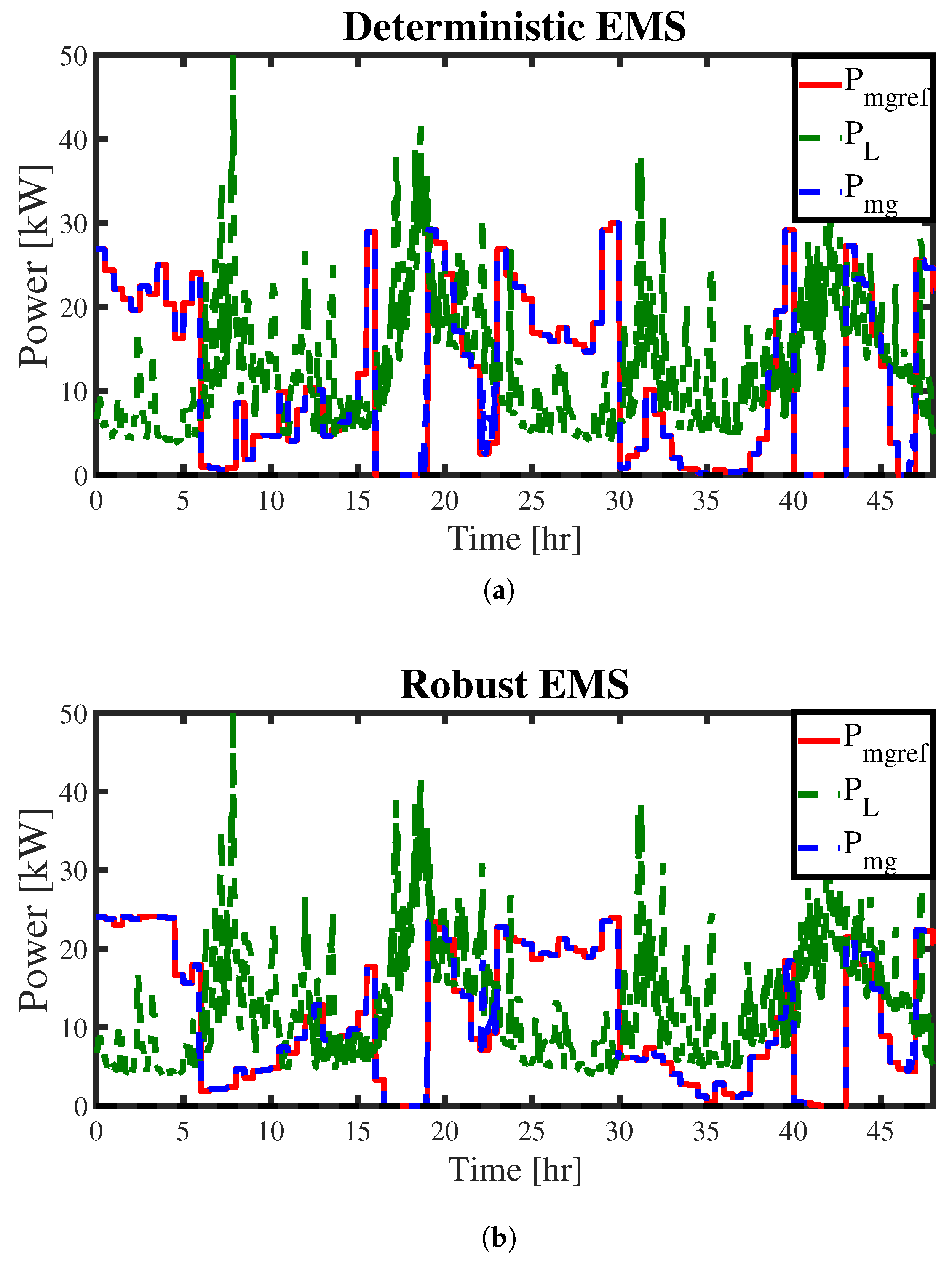
5.2. Hierarchical EMS Results
6. Conclusions
Author Contributions
Funding
Conflicts of Interest
Abbreviations
| EMS | Energy management system |
| MPC | Model predictive control |
| DNO | Distribution network operator |
| DER | Distributed energy resource |
| DG | Distributed generation |
| DN | Distribution network |
| ESS | Energy storage system |
| SoC | State of charge |
| PICP | Prediction interval coverage probability |
| PINAW | Prediction interval normalized average width |
| RMSE | Root mean square error |
| MAE | Mean absolute error |
| EFC | Equivalent full cycles |
| LPSP | Loss of power supply probability |
| LF | Load Factor |
| LLF | Load loss factor |
| MPD | Maximum power derivative |
| APD | Average power derivative |
Appendix A. Performance Indices for the Power Profile of the Main Grid
References
- Padhi, P.P.; Pati, R.K.; Nimje, A.A. Distributed generation: Impacts and cost analysis. Int. J. Power Syst. Oper. Energy Manag. 2012, 1, 91–96. [Google Scholar]
- Hidalgo, R.; Abbey, C.; Joós, G. A review of active distribution networks enabling technologies. In Proceedings of the IEEE PES General Meeting, Providence, RI, USA, 25–29 July 2010; pp. 1–9. [Google Scholar] [CrossRef]
- Abapour, S.; Zare, K.; Mohammadi-Ivatloo, B. Dynamic planning of distributed generation units in active distribution network. IET Gener. Transm. Distrib. 2015, 9, 1455–1463. [Google Scholar] [CrossRef]
- Palizban, O.; Kauhaniemi, K.; Guerrero, J.M. Microgrids in active network management—Part II: System operation, power quality and protection. Renew. Sustain. Energy Rev. 2014, 36, 440–451. [Google Scholar] [CrossRef]
- Mirzania, P.; Andrews, D.; Ford, A.; Maidment, G. Community Energy in the UK: The End or the Beginning of a Brighter Future? In Proceedings of the 1st International Conference on Energy Research and Social Science, Sitges, Spain, 5–7 April 2017. [Google Scholar]
- Lefroy, J. Local Electricity Bill. Available online: https://powerforpeople.org.uk/wp-content/uploads/2019/03/Local-Electricity-Bill.pdf (accessed on 3 October 2019).
- Fazeli, A.; Sumner, M.; Johnson, M.C.; Christopher, E. Real-time deterministic power flow control through dispatch of distributed energy resources. IET Gener. Transm. Distrib. 2015, 9, 2724–2735. [Google Scholar] [CrossRef]
- Daud, A.K.; Ismail, M.S. Design of isolated hybrid systems minimizing costs and pollutant emissions. Renew. Energy 2012, 44, 215–224. [Google Scholar] [CrossRef]
- Hosseinzadeh, M.; Salmasi, F.R. Power management of an isolated hybrid AC/DC microgrid with fuzzy control of battery banks. IET Renew. Power Gener. 2015, 9, 484–493. [Google Scholar] [CrossRef]
- Arcos-Aviles, D.; Pascual, J.; Marroyo, L.; Sanchis, P.; Guinjoan, F. Fuzzy Logic-Based Energy Management System Design for Residential Grid-Connected Microgrids. IEEE Trans. Smart Grid 2018, 9, 530–543. [Google Scholar] [CrossRef]
- Davies, R.; Sumner, M.; Christopher, E. Energy storage control for a small community microgrid. In Proceedings of the 7th IET International Conference on Power Electronics, Machines and Drives, Manchester, UK, 8–10 April 2014; pp. 1–6. [Google Scholar] [CrossRef]
- Silvente, J.; Kopanos, G.M.; Pistikopoulos, E.N.; Espuña, A. A rolling horizon optimization framework for the simultaneous energy supply and demand planning in microgrids. Appl. Energy 2015, 155, 485–501. [Google Scholar] [CrossRef]
- Palma-Behnke, R.; Benavides, C.; Lanas, F.; Severino, B.; Reyes, L.; Llanos, J.; Sáez, D. A Microgrid Energy Management System Based on the Rolling Horizon Strategy. IEEE Trans. Smart Grid 2013, 4, 996–1006. [Google Scholar] [CrossRef]
- Parisio, A.; Rikos, E.; Glielmo, L. A Model Predictive Control Approach to Microgrid Operation Optimization. IEEE Trans. Control Syst. Technol. 2014, 22, 1813–1827. [Google Scholar] [CrossRef]
- Olivares, D.E.; Cañizares, C.A.; Kazerani, M. A Centralized Energy Management System for Isolated Microgrids. IEEE Trans. Smart Grid 2014, 5, 1864–1875. [Google Scholar] [CrossRef]
- Ji, Z.; Huang, X.; Xu, C.; Sun, H. Accelerated Model Predictive Control for Electric Vehicle Integrated Microgrid Energy Management: A Hybrid Robust and Stochastic Approach. Energies 2016, 9, 973. [Google Scholar] [CrossRef]
- Li, Z.; Zang, C.; Zeng, P.; Yu, H. Combined Two-Stage Stochastic Programming and Receding Horizon Control Strategy for Microgrid Energy Management Considering Uncertainty. Energies 2016, 9, 499. [Google Scholar] [CrossRef]
- Brandstetter, M.; Schirrer, A.; Miletić, M.; Henein, S.; Kozek, M.; Kupzog, F. Hierarchical Predictive Load Control in Smart Grids. IEEE Trans. Smart Grid 2017, 8, 190–199. [Google Scholar] [CrossRef]
- Shayeghi, H.; Shahryari, E.; Moradzadeh, M.; Siano, P. A Survey on Microgrid Energy Management Considering Flexible Energy Sources. Energies 2019, 12, 2156. [Google Scholar] [CrossRef]
- Lara, J.D.; Olivares, D.E.; Cañizares, C.A. Robust Energy Management of Isolated Microgrids. IEEE Syst. J. 2018, 1–12. [Google Scholar] [CrossRef]
- Wu, W.; Chen, J.; Zhang, B.; Sun, H. A Robust Wind Power Optimization Method for Look-Ahead Power Dispatch. IEEE Trans. Sustain. Energy 2014, 5, 507–515. [Google Scholar] [CrossRef]
- Khodaei, A. Provisional Microgrids. IEEE Trans. Smart Grid 2015, 6, 1107–1115. [Google Scholar] [CrossRef]
- Yi, J.; Lyons, P.F.; Davison, P.J.; Wang, P.; Taylor, P.C. Robust Scheduling Scheme for Energy Storage to Facilitate High Penetration of Renewables. IEEE Trans. Sustain. Energy 2016, 7, 797–807. [Google Scholar] [CrossRef]
- Malysz, P.; Sirouspour, S.; Emadi, A. An Optimal Energy Storage Control Strategy for Grid-connected Microgrids. IEEE Trans. Smart Grid 2014, 5, 1785–1796. [Google Scholar] [CrossRef]
- Valencia, F.; Collado, J.; Sáez, D.; Marín, L.G. Robust Energy Management System for a Microgrid Based on a Fuzzy Prediction Interval Model. IEEE Trans. Smart Grid 2016, 7, 1486–1494. [Google Scholar] [CrossRef]
- Du, Y.; Pei, W.; Chen, N.; Ge, X.; Xiao, H. Real-time microgrid economic dispatch based on model predictive control strategy. J. Mod. Power Syst. Clean Energy 2017, 5, 787–796. [Google Scholar] [CrossRef]
- Zhang, Y.; Fu, L.; Zhu, W.; Bao, X.; Liu, C. Robust model predictive control for optimal energy management of island microgrids with uncertainties. Energy 2018, 164, 1229–1241. [Google Scholar] [CrossRef]
- Velarde, P.; Maestre, J.M.; Ocampo-Martinez, C.; Bordons, C. Application of robust model predictive control to a renewable hydrogen-based microgrid. In Proceedings of the 2016 European Control Conference (ECC), Aalborg, Denmark, 29 June–1 July 2016; pp. 1209–1214. [Google Scholar] [CrossRef]
- Pereira, M.; de la Peña, D.M.; Limon, D. Robust economic model predictive control of a community micro-grid. Renew. Energy 2017, 100, 3–17. [Google Scholar] [CrossRef]
- Fazeli, A.; Sumner, M.; Christopher, E.; Johnson, M. Power flow control for power and voltage management in future smart energy communities. In Proceedings of the 3rd Renewable Power Generation Conference, Naples, Italy, 24–25 September 2014; pp. 1–6. [Google Scholar] [CrossRef]
- Elkazaz, M.; Sumner, M.; Thomas, D. Real-Time Energy Management for a Small Scale PV-Battery Microgrid: Modeling, Design, and Experimental Verification. Energies 2019, 12, 2712. [Google Scholar] [CrossRef]
- Plett, G.L. High-performance battery-pack power estimation using a dynamic cell model. IEEE Trans. Veh. Technol. 2004, 53, 1586–1593. [Google Scholar] [CrossRef]
- Sun, F.; Xiong, R.; He, H.; Li, W.; Aussems, J.E. Model-based dynamic multi-parameter method for peak power estimation of lithium–ion batteries. Appl. Energy 2012, 96, 378–386. [Google Scholar] [CrossRef]
- Pérez, A.; Moreno, R.; Moreira, R.; Orchard, M.; Strbac, G. Effect of Battery Degradation on Multi-Service Portfolios of Energy Storage. IEEE Trans. Sustain. Energy 2016, 7, 1718–1729. [Google Scholar] [CrossRef]
- Der Merwe, R.V.; Wan, E.A. The square-root unscented Kalman filter for state and parameter-estimation. In Proceedings of the 2001 IEEE International Conference on Acoustics, Speech, and Signal Processing, Salt Lake City, UT, USA, 7–11 May 2001; Volume 6, pp. 3461–3464. [Google Scholar] [CrossRef]
- Tampier, C.; Pérez, A.; Jaramillo, F.; Quintero, V.; Orchard, M.; Silva, J. Lithium-ion battery end-of-discharge time estimation and prognosis based on Bayesian algorithms and outer feedback correction loops: A comparative analysis. In Proceedings of the Annual Conference of the Prognostics and Health Management Society, San Diego, CA, USA, 18–24 October 2015; Volume 6, pp. 182–195. [Google Scholar]
- Burgos, C.; Sáez, D.; Orchard, M.E.; Cárdenas, R. Fuzzy modelling for the state-of-charge estimation of lead-acid batteries. J. Power Sources 2015, 274, 355–366. [Google Scholar] [CrossRef]
- Pola, D.A.; Navarrete, H.F.; Orchard, M.E.; Rabié, R.S.; Cerda, M.A.; Olivares, B.E.; Silva, J.F.; Espinoza, P.A.; Pérez, A. Particle-Filtering-Based Discharge Time Prognosis for Lithium-Ion Batteries with a Statistical Characterization of Use Profiles. IEEE Trans. Reliab. 2015, 64, 710–720. [Google Scholar] [CrossRef]
- Sáez, D.; Ávila, F.; Olivares, D.; Cañizares, C.; Marín, L. Fuzzy Prediction Interval Models for Forecasting Renewable Resources and Loads in Microgrids. IEEE Trans. Smart Grid 2015, 6, 548–556. [Google Scholar] [CrossRef]
- Sáez, D.; Zuniga, R. Cluster optimization for Takagi & Sugeno fuzzy models and its application to a combined cycle power plant boiler. In Proceedings of the 2004 American Control Conference, Boston, MA, USA, 30 June–2 July 2004; Volume 2, pp. 1776–1781. [Google Scholar] [CrossRef]
- Babuška, R. Fuzzy Modeling for Control, 1st ed.; Kluwer Academic Publishers: Boston, MA, USA, 1998; p. 288. [Google Scholar] [CrossRef]
- Kouvaritakis, B.; Cannon, M. Model Predictive Control: Classical, Robust and Stochastic, 1st ed.; Springer: Berlin, Germany, 2016; p. 384. [Google Scholar] [CrossRef]
- Goulart, P.J.; Kerrigan, E.C.; Maciejowski, J.M. Optimization over state feedback policies for robust control with constraints. Automatica 2006, 42, 523–533. [Google Scholar] [CrossRef]
- Kouvaritakis, B.; Cannon, M.; Muñoz-Carpintero, D. Efficient prediction strategies for disturbance compensation in stochastic MPC. Int. J. Syst. Sci. 2013, 44, 1344–1353. [Google Scholar] [CrossRef]
- Richardson, I.; Thomson, M. One-Minute Resolution Domestic Electricity Use Data, 2008–2009. Colch. Essex UK Data Arch. 2010. [Google Scholar] [CrossRef]
- Green Energy UK. Tide—A New Way to Take Control; Green Energy UK: Ware, UK; Available online: https://www.greenenergyuk.com/Tide (accessed on 3 October 2019).
- Pascual, J.; Barricarte, J.; Sanchis, P.; Marroyo, L. Energy management strategy for a renewable-based residential microgrid with generation and demand forecasting. Appl. Energy 2015, 158, 12–25. [Google Scholar] [CrossRef]
- Parra, D.; Norman, S.A.; Walker, G.S.; Gillott, M. Optimum community energy storage for renewable energy and demand load management. Appl. Energy 2017, 200, 358–369. [Google Scholar] [CrossRef]
- Zahboune, H.; Zouggar, S.; Krajacic, G.; Varbanov, P.S.; Elhafyani, M.; Ziani, E. Optimal hybrid renewable energy design in autonomous system using Modified Electric System Cascade Analysis and Homer software. Energy Convers. Manag. 2016, 126, 909–922. [Google Scholar] [CrossRef]
- Bilal, B.O.; Sambou, V.; Ndiaye, P.A.; Kébé, C.M.F.; Ndongo, M. Multi-objective design of PV-wind-batteries hybrid systems by minimizing the annualized cost system and the loss of power supply probability (LPSP). In Proceedings of the 2013 IEEE International Conference on Industrial Technology (ICIT), Cape Town, South Africa, 25–28 Feburary 2013; pp. 861–868. [Google Scholar] [CrossRef]

| Hours | 00:00–06:00 | 06:00–16:00 | 16:00–19:00 | 19:00–23:00 | 23:00–24:00 |
|---|---|---|---|---|---|
| Energy Cost | 5 p/kWh | 12 p/kWh | 25 p/kWh | 12 p/kWh | 5 p/kWh |
| Performance Indices | Prediction Horizon | ||
|---|---|---|---|
| One Hour Ahead | Six Hours Ahead | One Day Ahead | |
| RMSE (kW) | 4.5136 | 5.0471 | 5.1974 |
| MAE (kW) | 3.2995 | 3.7316 | 3.7530 |
| PINAW (%) | 22.73 | 27.62 | 28.02 |
| PICP (%) | 88.22 | 89.79 | 89.83 |
| EMS Strategy | Cost | RMSE | EFC | LPSP |
|---|---|---|---|---|
| (£) | (kW) | Cycles | (%) | |
| Deterministic EMS | 168.01 | 1.22 | 6.40 | 3.780 |
| Robust EMS | 165.28 | 1.14 | 6.07 | 2.927 |
| EMS Strategy | C1 | C2 | C3 |
|---|---|---|---|
| (kWh) | (kWh) | (kWh) | |
| Deterministic | 990.361 | 934.338 | 25.483 |
| Robust | 994.081 | 931.231 | 15.321 |
| EMS Strategy | LF | LLF | MPD | APD | ||
|---|---|---|---|---|---|---|
| (kW) | (kW) | (kW/min) | (kW/min) | |||
| Deterministic | 0.3869 | 0.2452 | 30.00 | 0 | 29.63 | 0.1889 |
| Robust | 0.4459 | 0.2880 | 25.90 | 0 | 22.48 | 0.1318 |
© 2019 by the authors. Licensee MDPI, Basel, Switzerland. This article is an open access article distributed under the terms and conditions of the Creative Commons Attribution (CC BY) license (http://creativecommons.org/licenses/by/4.0/).
Share and Cite
Marín, L.G.; Sumner, M.; Muñoz-Carpintero, D.; Köbrich, D.; Pholboon, S.; Sáez, D.; Núñez, A. Hierarchical Energy Management System for Microgrid Operation Based on Robust Model Predictive Control. Energies 2019, 12, 4453. https://doi.org/10.3390/en12234453
Marín LG, Sumner M, Muñoz-Carpintero D, Köbrich D, Pholboon S, Sáez D, Núñez A. Hierarchical Energy Management System for Microgrid Operation Based on Robust Model Predictive Control. Energies. 2019; 12(23):4453. https://doi.org/10.3390/en12234453
Chicago/Turabian StyleMarín, Luis Gabriel, Mark Sumner, Diego Muñoz-Carpintero, Daniel Köbrich, Seksak Pholboon, Doris Sáez, and Alfredo Núñez. 2019. "Hierarchical Energy Management System for Microgrid Operation Based on Robust Model Predictive Control" Energies 12, no. 23: 4453. https://doi.org/10.3390/en12234453
APA StyleMarín, L. G., Sumner, M., Muñoz-Carpintero, D., Köbrich, D., Pholboon, S., Sáez, D., & Núñez, A. (2019). Hierarchical Energy Management System for Microgrid Operation Based on Robust Model Predictive Control. Energies, 12(23), 4453. https://doi.org/10.3390/en12234453


