Single-Phase 13-Level Power Conditioning System for Peak Power Reduction of a High-Speed Railway Substation

Abstract

The control and operation of a single-phase 13-level power conditioning system (PCS) for peak power reduction of a high-speed railway substation (HSRS) are proposed. This PCS is a single-phase 3100 V, 2 MVA 13-level H-bridge multi-level inverter structure. It has excellent power quality. It is easy to serialize by voltage. In addition, the DC bus power of each cell inverter is supplied by lithium-ion batteries. The generalized reduction gradient optimization algorithm based on past load pattern is applied to the power management system for peak power reduction of HSRS. The phase detector and power controller for the control of a single-phase PCS based on virtually coordinated axes using an all-pass filter are expected to be robust to external disturbances with fast response characteristics. This study also proposes an adapted select switch (ASS) method that can change the switching depending on the operation state of PCS and the state of charge (SOC) of the battery to minimize battery imbalance by controlling each cell inverter of the H-bridge. The validity of the proposed system was confirmed by PSiM simulation and experiments using a demonstration system of 6 MW PCS and 2.68 MWh batteries at one of Gyeongbu high-speed line substations in Korea.

1. Introduction

With the increase of traffic volume and traffic congestion due to industrial development and urban population concentration, measures to solve traffic problems are seriously highlighted. In this situation, electric railways have been proposed as the best alternative to solve transportation problems due to their advantages of being environmentally friendly, high energy use efficiency, safe, fast and convenient.

The demand for high-speed trains is continuously increasing due to their fast and convenient advantages. Therefore, railroad companies are increasing the number of rail operations to meet increasing demand. However, the increase in the number of trains causes problems of serious voltage drop and no margin for power supply capacity of high-speed railway substations (HSRSs) [1,2]. This peak power not only increases the electricity bill of the substation, but also adversely affects the stability of the power supply, such as voltage drop on the feed line [3].

Therefore, various studies have been performed to stabilize the high-speed railway power system. The optimal scheduling by adjusting the operation time and pattern of trains on the supply line has been highlighted as a way to use energy efficiently without any special cost investments [4]. However, it is not easy to find an optimal pattern because there are various variables depending on driving habits of locomotive engineers and sudden occurrences of train stations. For voltage stabilization, reactive power compensation methods using the power quality compensators, such as a static var compensator (SVC) or an active power filter (APF), have been applied [5,6,7]. With these methods, the investment cost of facilities is relatively low. However, the power compensation is limited due to the limitation of devices supplied by reactive power only. To supply the active power, energy storage systems have been proposed to install on board [8] or at the substation and section-post [9,10,11,12]. Although the on-board system has the advantage of optimally utilizing the regenerative energy by mounting an energy storage device on the vehicle, it has disadvantages of increasing the weight of the vehicle and constraining the installation space [13,14]. For this reason, installing energy storage systems at the station using high-power and large capacity energy storage systems (ESSs), such as a flywheel [10], electric double layer capacitors (EDLCs) [11], or Li-ion batteries [12], has been considered.

In general substations, ESSs are usually installed in three-phase systems for the purpose of peak power reduction and power stabilization [15,16,17]. However, these systems could not apply directly to special loads, such as HSRSs; because HSRSs use a high-voltage large-power single-phase power system, load fluctuations are much greater than normal loads [18]. To respond to these load characteristics, it is necessary to study the ESS suitable for load characteristics of HSRS.

In this paper, a single-phase 13-level power conditioning system (PCS) for peak power reduction of HSRS is proposed. ESSs using Li-ion batteries with high power and high energy density are considered to meet the load characteristics of HSRS. The ESS for HSRS consists of a power management system (PMS) for power operation, a PCS for power control, and batteries for energy storage. Among them, the PMS uses the generalized reduction gradient (GRG) optimization algorithm based on the past load pattern instead of using the slope detection method by the differentiator to reduce the peak power of the general consumer for special loads of HSRS [19,20]. In addition, the PCS is configured as a 13-level single-phase H-bridge-type inverter to overcome the AC output voltage limit of PCS from the series maximum voltage of the battery, thereby reducing the electromagnetic interference (EMI) due to dv/dt components and improving the total harmonic distortion (THD) characteristics and efficiency [20].

The phase detector and power controller for the control of a single-phase PCS based on virtually coordinated axes using an all-pass filter are proposed in this study to be robust to external disturbances with fast response characteristics. This study also proposes a control technique to minimize battery imbalance by controlling the battery separated by each cell inverter of the H-bridge-type PCS depending on the battery condition and the operating condition of PCS. The validity of the proposed system including the dynamic characteristics of the controller, the output voltage regulation, and the THD characteristics of the current were confirmed through PSiM simulations. Furthermore, the effectiveness and the feasibility of the proposed system were verified by installing a demonstration system of 6 MW PCS and 2.68 MWh batteries at one of Gyeongbu high-speed line substations in Korea in an actual operation.

2. Peak Power Reduction System for High-Speed Railway Substations

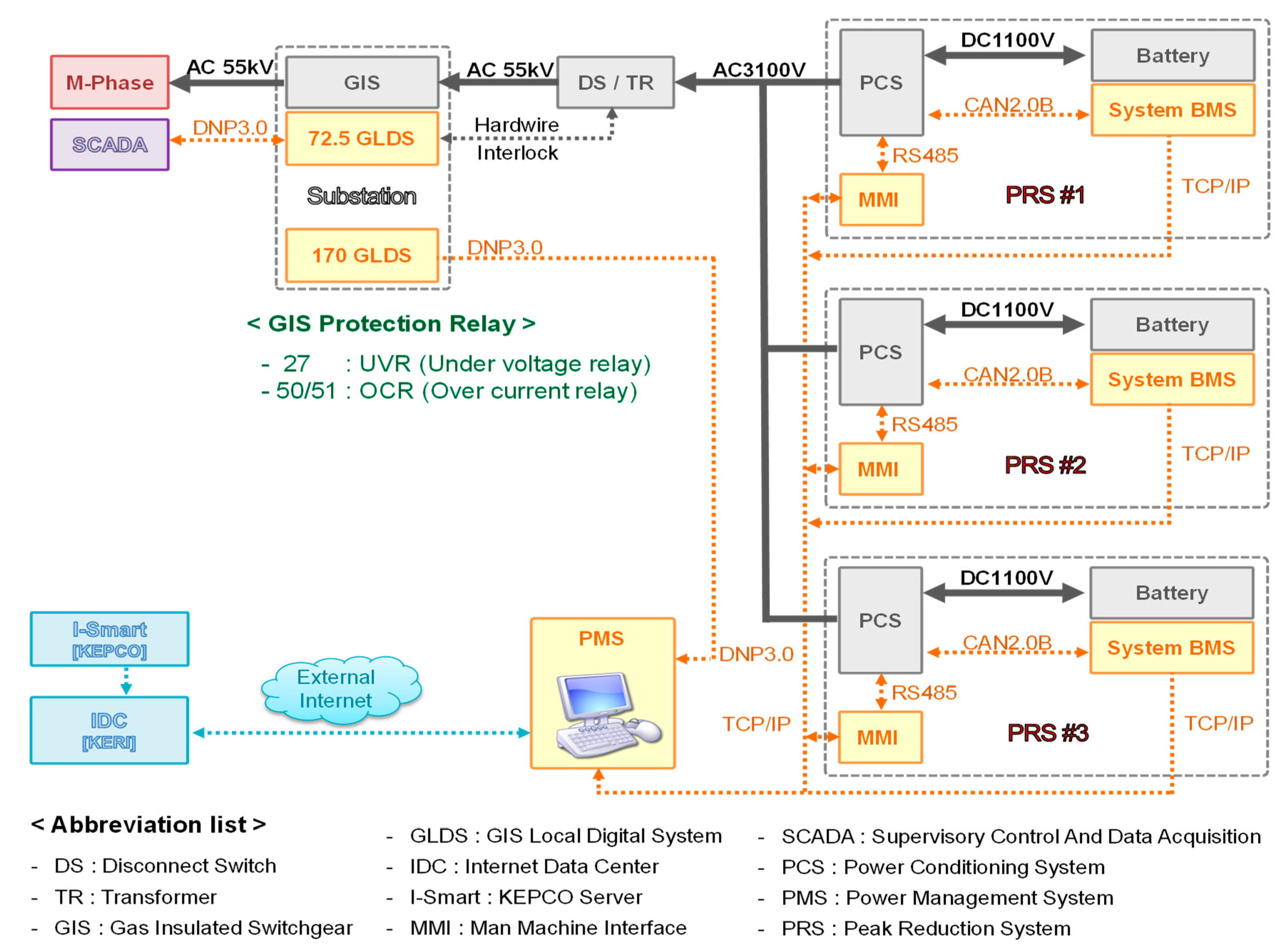
Figure 1 shows the configuration of the peak power reduction system (PPRS) for HSRS. It is linked to a 55 kV supply line to perform the function of reducing peak power and stabilizing catenary voltage. The PPRS consists of a PMS, a PCS, and batteries. The PMS is responsible for monitoring the catenary condition and for protecting the cooperation system with the substation. The PCS controls the power as a power command given by the PMS. On the other hand, the battery performs the function of energy storage and transmits the battery state to the PMS via the battery management system (BMS).

2.1. Power Management System

In general, high-speed trains run according to a pre-determined schedule. Thus, they show relatively regularized load patterns on every day of the week. However, load patterns can be changed due to delays of passengers’ boarding and train operation as well as the formation of temporary trains. Therefore, to reduce the peak load of HSRS, a future ESS operation plan has to be established optimally by predicting load patterns as accurately as possible [21].

Figure 2 shows the optimization algorithm of the ESS operation for peak power reduction using load prediction techniques [22].

To analyze daily load prediction patterns, past data were collected for three weeks and groups of candidates for peak power were chosen among 96 sections of 15 min duration per day. After this, charging and discharging sections were determined by applying the objective function to reduce the peak power among the peak power candidate groups. The objective function is set to minimize the charging cost of the daily ESS and the sum of peak reduction of the discharge interval, as in Equation (1).

$$F={\displaystyle \sum }_{i=1}^{96}\left(E{O}_i\times C_i\right)+P{L}_i$$

(1)

where, $i$ is an each section number of the daily peak power calculation interval for 15 min,$E{O}_i$ is the amount of PCS charging or discharging energy for section $i$, which is a plus sign in charging and a negative sign in discharging,$C_i$ is the electric charge rate at section $i$, and $P{L}_i$ is the saved electric charge through peak power reduction.

The battery daily charge/discharge plan obtained from the objective function reflects the constraints and establishes the final optimization plan. The constraints are PCS operation interval, upper and lower ranges of the battery SOC, and upper and lower ranges of supply power. The mathematical models for optimization with constraints are solved by using the generalized reduced gradient (GRG) algorithm.

Figure 3 shows the simulated results of PMS when the daily operation plan of ESS based on the predicted load is applied to the actual load data. According to the analysis of the substation power for some past years, the peak power generated by the substation is analyzed to be about 30 MW. Therefore, the target peak power of the substation is set to 24 MW under the assumption that the capacity of the peak reduction system is 6 MW PCS with 2.68 MWh battery when the PMS simulation is performed.

The simulation results showed that the peak power generation of the substation was accurately predicted at 09:30 AM through the load prediction algorithm of the PMS. Therefore, the peak power generated by the substation was managed at 23.926 MW by supplying 6 MW power from the PCS. If the PMS failed to predict the load, the peak power generated from the substation might be approximately 30 MW.

2.2. Battery and Battery Management System

Batteries applied to the development of peak reduction devices for HSRS are designed to install in 40 ft containers, consisting of trays, racks, and banks with lithium-ion batteries. In the container, each of the six banks are insulated so that they can be connected to each cell inverter in the PCS. Batteries connected to the 2 MW PCS are installed with a capacity of 149 kWh for each bank with a total capacity of 894 kWh.

Table 1. Specifications by Battery Configuration.

	Specification
	Tray	Rack	Bank	System
Energy (kWh)	3.55	49.7	149	894
Capacity (Ah)	60	60	180	1080
Operating Voltage (V)	48.0–65.6	672–918.4	672–918.4	672–918.4
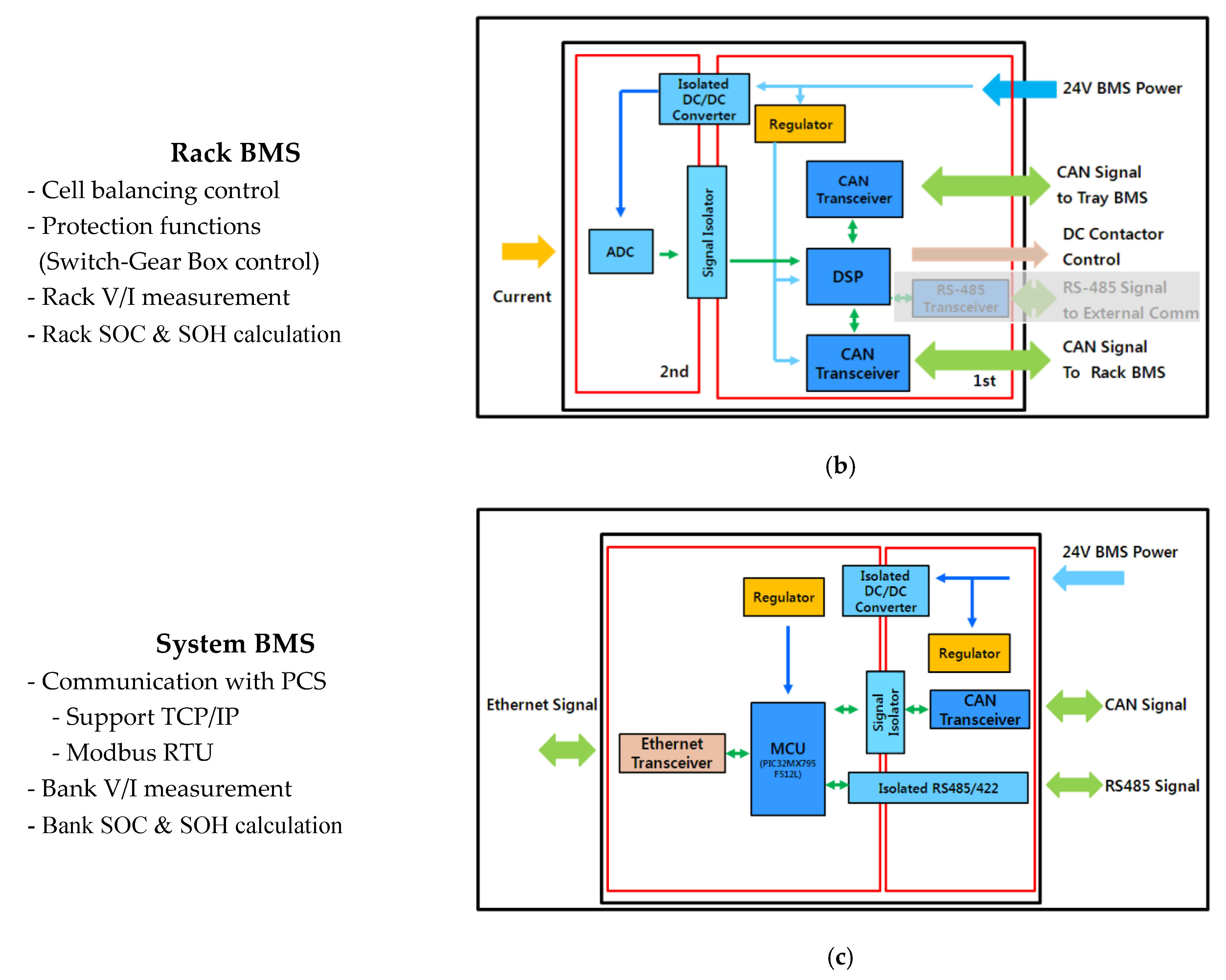
Cell Configuration	16P1P (16 Cell)	224S1P (14 Tray)	224S3P (3 Rack)	224S18P (6 Bank)

shows the specifications of each battery unit. In addition, monitoring and managing battery condition is performed through the battery management system (BMS). As shown in Figure 4, the BMS is also installed with a tray, rack, and system to match the battery configuration. The tray BMS collects the condition of the battery on a cell basis. The collected data is managed through the rack BMS. The system BMS also collects information from each rack BMS, compiles the information in bank units, and transmits it to the PCS and PMS in real time.

2.3. Power Conditioning System (PCS)

The PCS applied to the development of the peak power reduction system for HSRS is connected in parallel to a single-phase 55 kV supply line. It controls the power according to the schedule of the charging and discharging power operation optimized by PMS. The H-bridge-type multilevel inverter method is applied for PCS to overcome the voltage limit of AC output by battery serial configuration voltage, thereby improving the system efficiency and output characteristics [23,24].

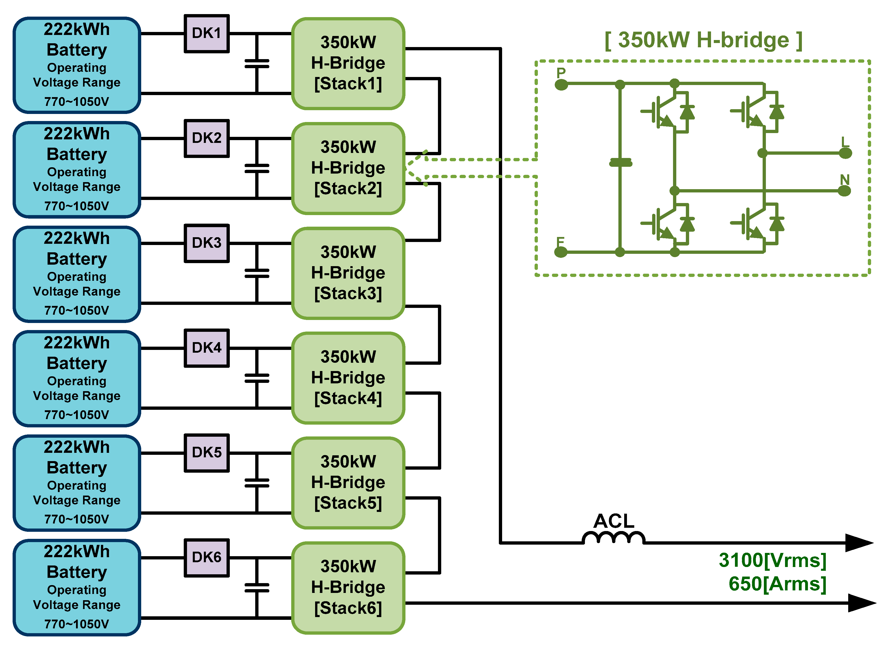
The applied PCS consists of a single phase 13-level H-bridge-type multilevel inverter using six separate battery banks, as shown in Figure 5. The PCS hardware is designed so that the main circuit of each cell inverter can be separated into a plug-in type. The control method of multi-level inverter adopts an intensive control method based on hardwire instead of a distributed control method through the communication interface, as shown in Figure 6, thus enhancing the stability and reliability of the system. In addition, the phase disposition (PD) PWM method is chosen for the modular multi-level converter (MMC) to get the best THD characteristics [25]. A three-level switching is applied for each cell inverter using the unipolar PWM technique.

Table 2. Comparison of Specification between the Proposed PCS and the Existing One.

	Existing PCS	Proposed PCS
Connection	Three phase	Single phase
Capacity	Maximum 2 MW	2 MW
Output voltage	380 Vrms or 440 Vrms	3100 Vrms
Battery voltage	Maximum 1050 V	Maximum 1050 V
THD	2–3%	Less than 1%
Topology	2-level, 3-level NPC *	13-level Cascade
Scalability	Parallel extension	Parallel extension Series extension
Demand forecast	Slope detection by demand controller	Data-based learning

* NPC: Neutral point Clamped.

shows the comparison of specifications between the existing PCS and the proposed one. Unlike conventional techniques, the proposed PCS was designed to be suitable for single-phase high-voltage large capacity customers.

3. PCS Controller Design

Controllers for the single-phase 13-level multi-level PCS consist of a phase detection controller for voltage sensing of the catenary, a power controller for power control, and a balancing controller for optimal utilization of batteries separated by a cell inverter. In this paper, controllers are designed using virtual coordinate axes to improve the dynamic characteristics of phase detection controllers and power controllers on the single-phase system. This paper also uses a battery balancing control technique that allows the battery separated by each cell inverter to distribute power according to the SOC of batteries and PCS operating conditions.

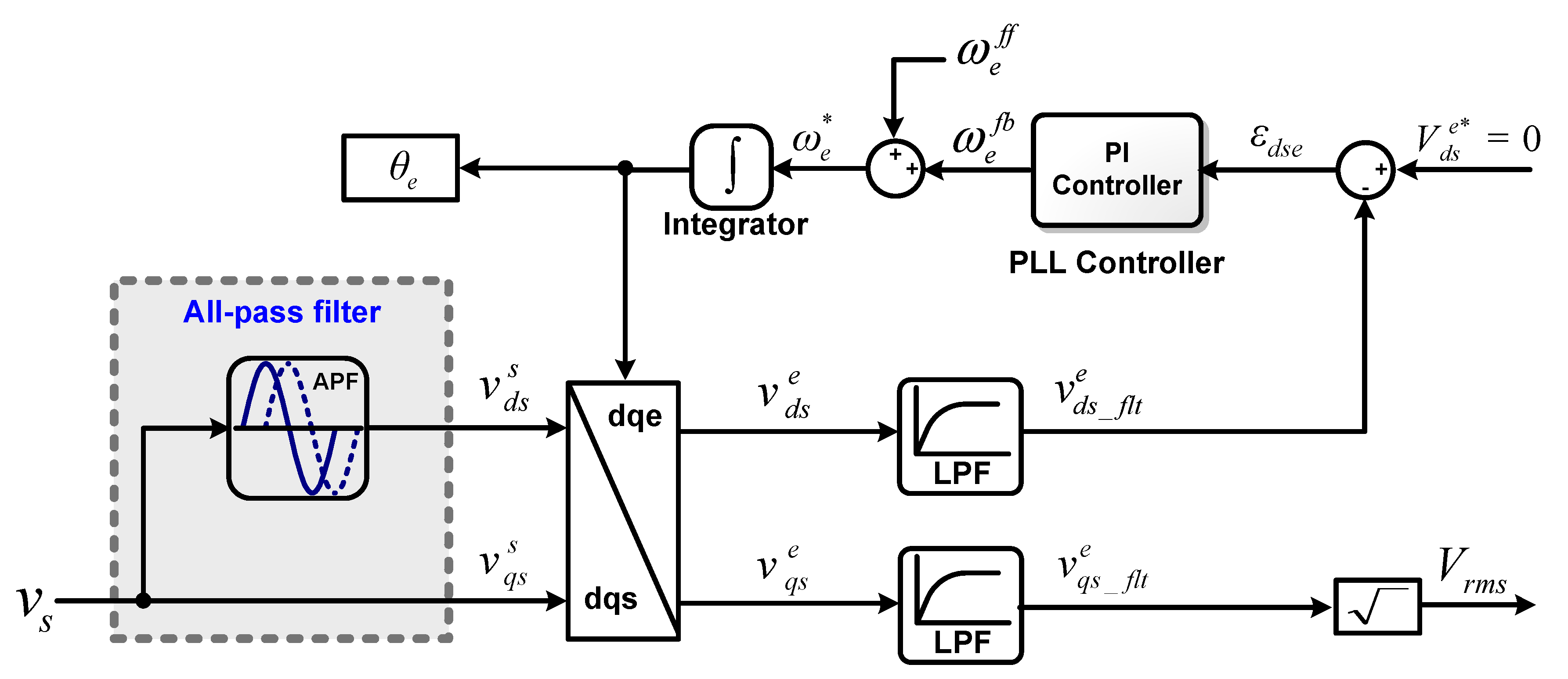
3.1. Single-Phase Synchronous Reference Frame-Phase Locked Loop (SRF-PLL) Controller

The PCS connected to the single-phase 55 kV power line shall provide power by accurately identifying the voltage phase information of the catenary. Normally, the synchronous reference frame-phase locked loop (SRF-PLL) technique is applied to the three-phase power system, which detects the voltage phase angle through the synchronous coordinate transformation from the measured voltage [26,27]. In this paper, to apply the SRF-PLL technique to the single-phase system, the all-pass filter (APF) method is used to detect the voltage phase angle.

In particular, a low-pass filter (LPF) was applied to the voltage converted into a synchronous reference frame for stable phase detection and reduced disturbance so that the response characteristics of PLL could be improved and its stability could be ensured [28].

Figure 7 shows a block diagram of a single-phase SRF-PLL phase angle detector. The single-phase input voltage, $v_s$, can be determined with Equation (2).

$$v_s=v_{qs}^s =V_s\sin {\omega }_{e}t$$

(2)

where, $v_{qs}^s$ is the q-axis voltage at the d–q stationary coordinate system.

Applying APF, as in Equation (3), $v_{ds}^s,$ the orthogonal component of $v_{qs}^s$ can be obtained with Equation (4).

$$K{\left(s\right)}_{APF}=\frac{s-\omega }{s+\omega }$$

(3)

$$v_{ds}^s=k\left(t\right)v_{qs}^s=V_s\cos {\omega }_{e}t$$

(4)

The d–q synchronous coordinate transformation from Equations (2) and (4) can be calculated using Equation (5). As a result, $v_{ds}^e$ and $v_{qs}^e$ are calculated as shown in Equation (6).

$$\left[\begin{array}{c}{v}_{ds}^e\\ v_{qs}^e\end{array}\right]=\left[\begin{array}{cc} \cos {\omega }_{e}t& \sin {\omega }_{e}t\\ -\sin {\omega }_{e}t& \cos {\omega }_{e}t\end{array}\right]\left[\begin{array}{c}{v}_{ds}^s\\ v_{qs}^s\end{array}\right]$$

(5)

$$v_{ds}^e=0, v_{qs}^e=V_s$$

(6)

If the phase angle of the voltage can be accurately known, the d-axis voltage $v_{ds}^e$ becomes zero and the q-axis voltage $v_{qs}^e$ becomes the magnitude of the voltage, as shown in Equation (6).

The controller is configured as shown in Figure 7 so that the d-axis voltage is zero due to this relationship. In the block diagram shown in Figure 7, if the phase angle range is small enough, it can be $\sin {\theta }_e\cong {\theta }_e$. For this reason, the error of the d-axis voltage can be linearized to the error of the phase angle. The block diagram in Figure 7 is modeled as a linearized control system with LPF, as shown in Figure 8.

From Figure 8, the transfer function of the PLL system is calculated with Equation (7), where $G{\left(s\right)}_{pll}$ and $K{\left(s\right)}_{LPF}$ are the open-loop transfer function and the low-pass filter transfer function, as shown in Equations (8) and (9), respectively.

$$H{\left(s\right)}_{pll}=\frac{G{\left(s\right)}_{pll}}{1+G{\left(s\right)}_{pll}K{\left(s\right)}_{LPF}}=\frac{V_s{K}_P\left[s^2+\left({\omega }_c+\frac{1}{\tau }\right)s+\frac{{\omega }_c}{\tau }\right]}{s^3+{\omega }_c{s}^2+V_s{K}_P{\omega }_{c}s+\frac{V_s{K}_P{\omega }_c}{\tau }}$$

(7)

$$G{\left(s\right)}_{pll}=V_s\left(K_P\frac{1+s\tau }{s\tau }\right)\frac{1}{s}$$

(8)

$$K{\left(s\right)}_{LPF}=\frac{{\omega }_c}{s+{\omega }_c}$$

(9)

where, $K_P$ is the proportional gain of the PI controller, τ is the time constant of the PI controller, and ${\omega }_c$ is the bandwidth of the low-pass filter.

Pole placement techniques are used to model the PLL closed loop transfer function of Equation (7) into a typical secondary control system.

Equation (7) may be expressed in the form of multiplication of the dominant pole and a typical secondary control system, as shown in Equation (10) [28,29].

$$H{\left(s\right)}_{pll}\cong \frac{\left(s+k\right)}{\left(s+k\right)} \frac{As+B}{s^2+2\zeta {\omega }_{n}s+{\omega }_n^2}=\frac{A{s}^2+\left(kA+B\right)s+kB}{s^3+\left(2\zeta {\omega }_n+k\right)s^2+\left(2\zeta {\omega }_{n}k+{\omega }_n^2\right)s+k{\omega }_n^2}$$

(10)

where ζ is the damping ratio and ${\omega }_n$ is the bandwidth of the typical secondary system.

Equations (11) and (12) can be calculated by assuming that Equation (10) has a dominant pole of k = 1 and applying the coefficient comparison method from the characteristic equation of Equations (7) and (10).

$${\omega }_c=1+2\zeta {\omega }_n$$

(11)

$$K_p=\frac{2\zeta {\omega }_n+{\omega }_n^2}{V_s{\omega }_c}, \tau =\frac{K_p{V}_s{\omega }_c}{{\omega }_n^2}$$

(12)

Setting the bandwidth ${\omega }_n$ and damping ratio ζ of the typical secondary system gives the bandwidth of the low-pass filter and the optimized gain of the PI control. Empirically, the cutoff frequency of LPF, ${\omega }_c$, is determined from 100 to 300 rad/s. For applying to the PCS, the bandwidth and damping ratio are chosen as 100 rad/s and 0.75 respectively, to meet ${\omega }_c$ to be 150 rad/s.

3.2. Power Controller

Definitions of electric power for the single-phase in the sinusoidal system have been well established. For an ideal single-phase system with a sinusoidal voltage source and a linear load, the voltage and current are represented by Equation (13).

$$v_s=V_s\sin {\omega }_{e}t,\dots , i_s=I_s\sin \left({\omega }_{e}t+\varphi \right)$$

(13)

where $V_s$ and $I_s$ represent the peak values of the voltage and current.

The instantaneous power is given by the product of the instantaneous voltage and current, as shown in Equation (14).

$$p_s=v_s{i}_s=V_s I_s\sin \left({\omega }_{e}t\right)\sin \left({\omega }_{e}t+\varphi \right)=\frac{1}{2}{V}_s I_s\left[\cos \varphi -\cos \left(2{\omega }_{e}t+\varphi \right)\right]$$

(14)

Equation (14) shows that the instantaneous power of the single-phase system is not constant. It has an oscillating component at twice the line frequency with the average value of $\frac{1}{2}{V}_s I_s\cos \varphi$. Decomposition of the oscillating component and rearrangement of Equation (14) yields the following Equation (15), with two terms which derive the traditional concept of active and reactive power [30].

$$\begin{gathered} p_s=\frac{1}{2}{V}_s I_s\cos \varphi \left[1-\cos 2{\omega }_{e}t\right]-\frac{1}{2}{V}_s I_s\sin \varphi \sin 2{\omega }_{e}t \\ =P\left[1-\cos 2{\omega }_{e}t\right]-Q\sin 2{\omega }_{e}t \end{gathered}$$

(15)

where $P$ and $Q$ represent active and reactive powers, respectively.

In general, the power of the three-phase system can be analyzed through the d–q synchronous transformation, as shown in Equation (16) [31,32].

$$\begin{array}{c}P=\frac{1}{2}\left( v_{ds}^e i_{ds}^e+v_{qs}^e i_{qs}^e \right)=\frac{1}{2} v_{qs}^e i_{qs}^e\\ Q=\frac{1}{2}\left(-v_{ds}^e i_{qs}^e+v_{qs}^e{i}_{ds}^e\right)=\frac{1}{2} v_{qs}^e i_{ds}^e\end{array}$$

(16)

where $v_{ds}^e$,$v_{qs}^e$, $i_{ds}^e$, and $i_{qs}^e$ are the d-q synchronous transformation of the input voltage, $v_s$, and current, $i_s$.

For a single-phase system, it is possible to calculate power applying Equation (16) by calculating the voltage and current orthogonal components using an all-pass filter. In addition, the $v_{ds}^e$ can be calculated as ‘0′, which is the phase reference value of the system voltage.

The power in the single-phase system can be verified, as shown in Equation (17), to enable the control of active and reactive powers through d-axis and q-axis currents.

$$i_{qs}^{e\ast }=\frac{2P^{\ast }}{v_{qs}^{e\ast }}, i_{ds}^{e\ast }=\frac{2Q^{\ast }}{v_{qs}^{e\ast }}$$

(17)

where, $P^{\ast }$ is the active power command, $Q^{\ast }$ is the reactive power command, $I_{ds}^{e\ast }$ is the d-axis current command, and $I_{qs}^{e\ast }$ is the q-axis current command.

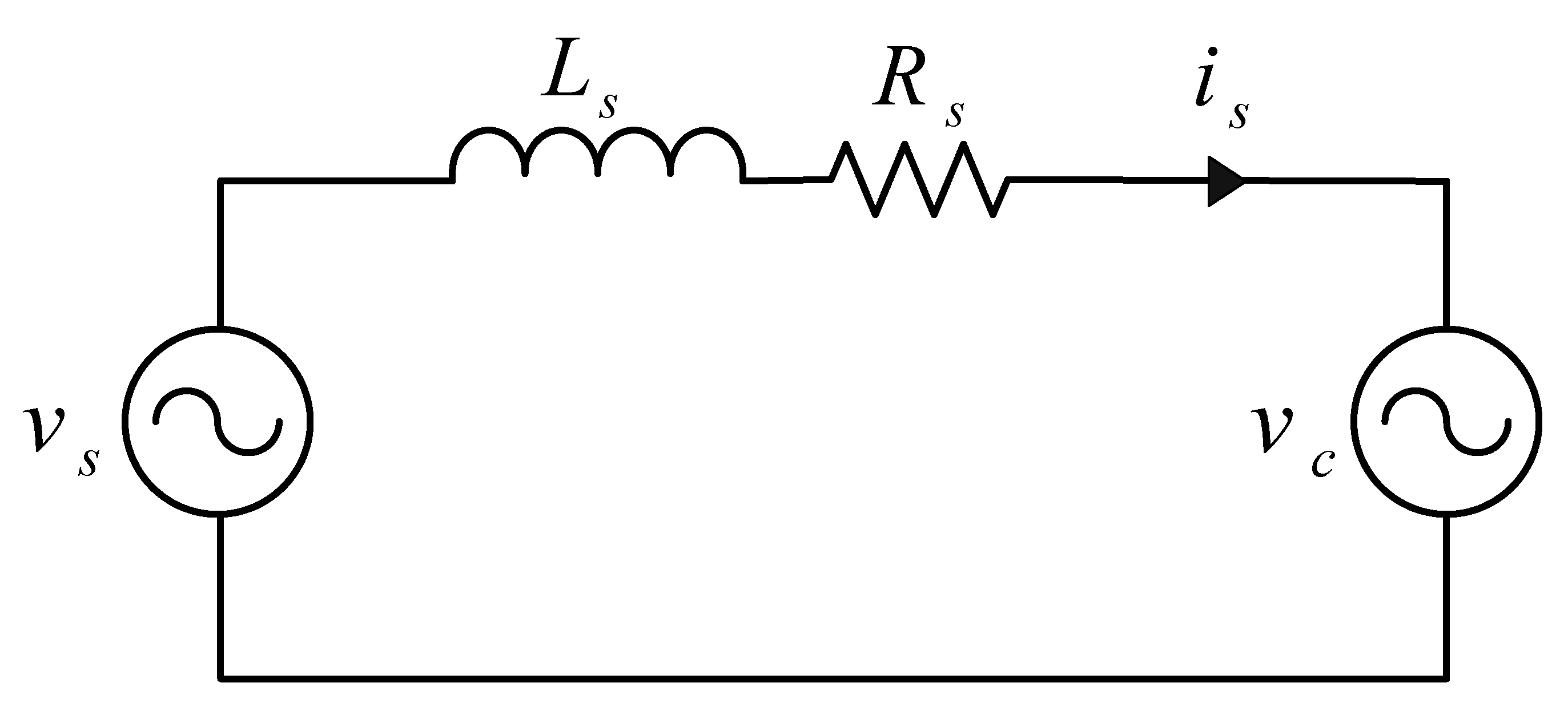
3.3. Current Controller

Figure 9 shows the equivalent circuit of a single-phase PCS system, where $v_s$ is the source voltage, $v_c$ is the generated voltage of PCS, $i_s$ is the generated current of PCS, and $L_s$ and $R_s$ are the reactance and resistance of the source and filter reactor. The voltage equation of the equivalent circuit shown in Figure 9 is shown in Equation (18).

$$L_s\frac{d{i}_s}{dt}+R_s{i}_s=v_s-v_c$$

(18)

Equation (18) in the d-q synchronous coordinate system can be expressed as shown in Equation (19).

$$\begin{gathered} L_s\frac{d}{dt}\left[\begin{array}{c}i{ }_{ds}^e\\ i{ }_{qs}^e\end{array}\right]+R_s\left[\begin{array}{c}i{ }_{ds}^e\\ i{ }_{qs}^e\end{array}\right]=\left[\begin{array}{c}{v}_{ds}^e\\ v_{qs}^e\end{array}\right]-\left[\begin{array}{c}{v}_{cd}^e\\ v_{cq}^e\end{array}\right]+{\omega }_e{L}_s\left[\begin{array}{c}-i{ }_{qs}^e\\ i{ }_{ds}^e\end{array}\right] \\ \frac{d}{dt}\left[\begin{array}{c}i{ }_{ds}^e\\ i{ }_{qs}^e\end{array}\right]=\left[\begin{array}{cc}-R_s/L_s& 0\\ 0& -R_s/L_s\end{array}\right]\left[\begin{array}{c}i{ }_{ds}^e\\ i{ }_{qs}^e\end{array}\right]+\frac{1}{L_s}\left[\begin{array}{c}{v}_{ds}^e-v_{cd}^e-{\omega }_e{L}_s i{ }_{qs}^e\\ v_{qs}^e-v_{cq}^e+ {\omega }_e{L}_s i{ }_{ds}^e\end{array}\right] \end{gathered}$$

(19)

where, $v_{cd}^e$ is the d-axis voltage of the PCS, $v_{cq}^e$ is the q-axis voltage of the PCS, and $v_{ds}^e$ is 0.

If the intermediate variable $x_1$ and $x_2$ are defined as in Equation (20), Equation (19) can be expressed as Equation (21).

$$\{\begin{array}{c}{x}_1=-v_{cd}^e-{\omega }_e{L}_s i{ }_{qs}^e \\ x_2= v_{qs}^e-v_{cq}^e+ {\omega }_e{L}_s i{ }_{ds}^e\end{array}$$

(20)

$$\frac{d}{dt}\left[\begin{array}{c}i{ }_{ds}^e\\ i{ }_{qs}^e\end{array}\right]=\left[\begin{array}{cc}-R_s/L_s& 0\\ 0& -R_s/L_s\end{array}\right]\left[\begin{array}{c}i{ }_{ds}^e\\ i{ }_{qs}^e\end{array}\right]+\frac{1}{L_s}\left[\begin{array}{c}{x}_1\\ x_2\end{array}\right]$$

(21)

Variables $x_1$ and $x_2$ are obtained by Equation (22).

$$\{\begin{array}{c}{x}_1=k_P\left(i{ }_{ds}^{e\ast }-i{ }_{ds}^e\right)+k_I{\displaystyle \int }\left(i{ }_{ds}^{e\ast }-i{ }_{ds}^e\right)dt \\ x_2=k_P\left(i{ }_{qs}^{e\ast }-i{ }_{qs}^e\right)+k_I{\displaystyle \int }\left(i{ }_{qs}^{e\ast }-i{ }_{qs}^e\right)dt\end{array}$$

(22)

where $k_P$ and $k_I$ are the proportional gain and the integral gain of the PI controller, respectively.

Figure 10 shows a block diagram of the current controller. From Figure 10, the transfer function of the current controller is calculated, as shown in Equation (23).

$$H\left(s\right)=\frac{I_{dq}^e\left(s\right)}{I_{dq}^{e\ast }\left(s\right)}=\frac{\frac{\alpha k_P}{L_s}s+\frac{k_I}{L_s}}{s^2+\left(\frac{R_s+k_P}{L_s}\right)s+\frac{k_I}{L_s}}$$

(23)

where α is a parameter for selecting the PI or IP controller (α = 1 for PI and α = 0 for IP).

The advantage of the IP controller is that it is easy to set gains. However, the phase delay in the cut-off frequency band is 90°. On the other hand, for PI controllers, although there are some difficulties in setting gains due to the addition of zero to the transfer function, the phase delay is only 45°, thus showing better dynamic characteristics than the IP controller under similar gain.

In this paper, α is selected as ‘1′ to compose the PI current controller. The PI controller is very difficult to designate poles and zeroes as arbitrary values. Thus, it is relatively easy to establish stable gains by applying the ‘approximate gain setting’ [33].

This approach takes advantage of the fact that the closed loop transfer function appears as ${\omega }_{cc}/\left(s+{\omega }_{cc}\right),$ as shown in Equation (24), approximating the open loop transfer function to ${\omega }_{cc}/s$. At this point, the cross-over frequency at which the gain of the closed loop transfer function is ‘1’ is equal to ${\omega }_{cc}$.

$$H\left(s\right)=\frac{{\omega }_{cc}}{s+{\omega }_{cc}}$$

(24)

Calculation of the transfer function by Equations (23) and (24) is performed as shown in Equation (25). From the calculated equation, the gain value of the current controller by the coefficient comparison method can be obtained, as shown in Equation (26).

$$\left(s+{\omega }_{cc}\right)\left(\frac{k_P}{L_s}s+\frac{k_I}{L_s}\right)={\omega }_{cc}\left[s^2+\left(\frac{R_s+k_P}{L_s}\right)s+\frac{k_I}{L_s}\right]$$

(25)

$$k_P=L_s{\omega }_{cc} , k_I={\omega }_{cc}\left(k_P+R_s\right)+k_P$$

(26)

If the cross-over frequency, ${\omega }_{cc}$, is large, dynamic characteristics are great. Therefore, the quick response in transient condition may be obtained. However, due to the sensitivity of noise and disturbance in the system, it is necessary to select appropriate values. Empirically, it is determined between 750 to 1500 rad/s of LPF. In this study, LPF of 1200 rad/s is applied to the PCS current controller.

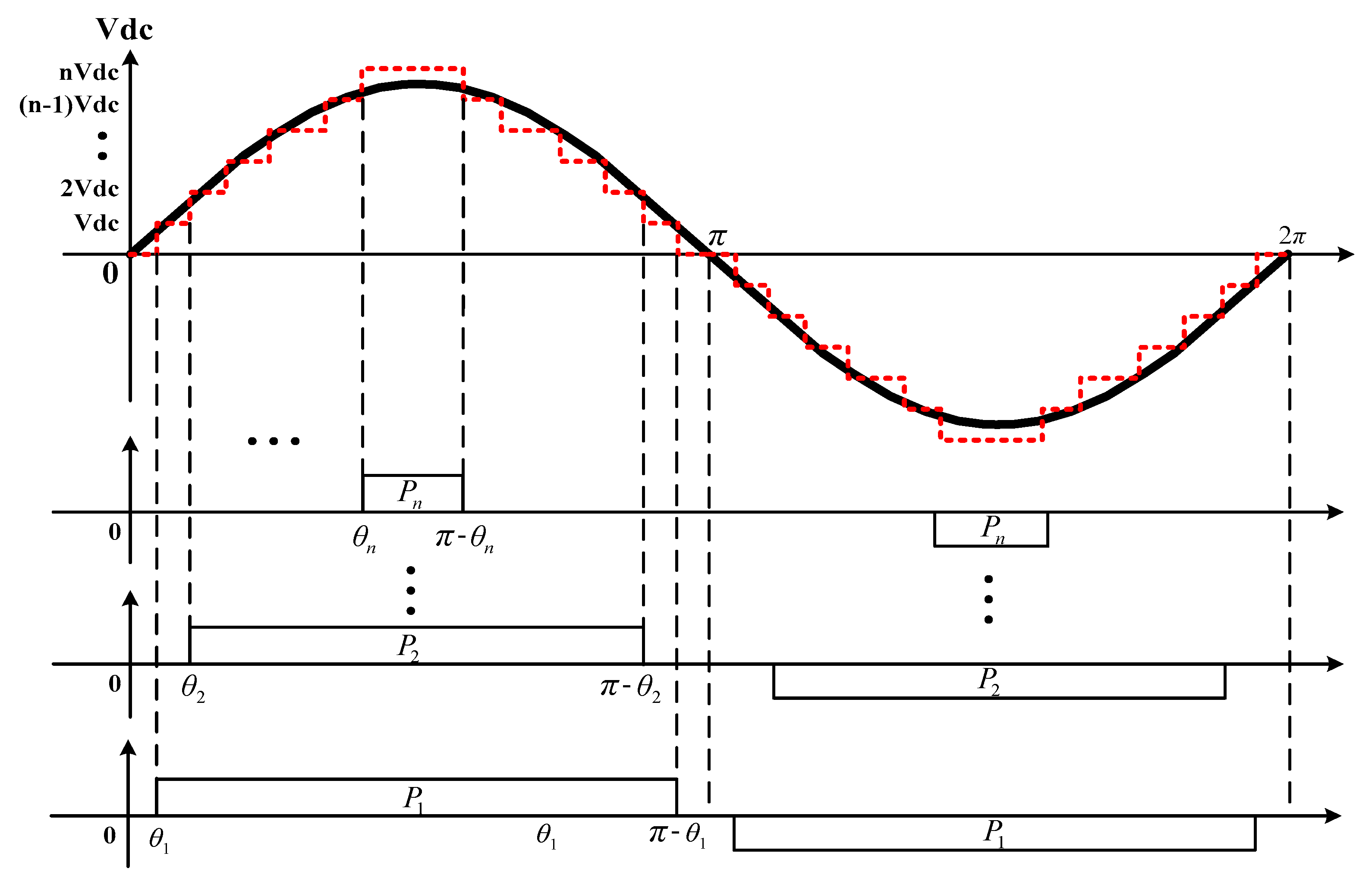
3.4. Multi-Level PWM Configuration

As shown in Figure 11, various modulation schemes can be applied for the switching of multi-level inverters depending on the purpose of use and the application area [34]. The H-bridge-type inverter is applied with a level-shifted method (LSM) to enable power distribution control as DC link power is used by the battery. It is also applied using the PD method with the best THD characteristics among LSM methods [35].

The cascade-type inverter consisting of an H-bridge has an output voltage, as shown in the red dotted line in Figure 12. The Fourier transform is calculated with Equation (27). In addition, the amount of power over one cycle of each cell inverter is distributed, as shown in Equation (28), by phase angles ${\theta }_1, {\theta }_2,\dots ,{\theta }_m$.

$$v_s\left(t\right)=\frac{4V_{dc}}{\pi } \frac{\sin n\omega t}{n}{\displaystyle \sum }_{n=1}^{\infty }\left(\cos n{\theta }_1+\cos n{\theta }_2+\dots +\cos n{\theta }_m\right)$$

(27)

$$E_{dc1}=4V_{dc}{I}_{dc}\left(\frac{\pi }{2}-{\theta }_1\right), E_{dc2}=4V_{dc}{I}_{dc}\left(\frac{\pi }{2}-{\theta }_2\right), E_{dcH}=4V_{dc}{I}_{dc}\left(\frac{\pi }{2}-{\theta }_m\right)$$

(28)

where ${\theta }_m$ is $\sin \frac{n}{m}$ and n is from 1 to m.

As shown in the results of Equation (28), the H-bridge-type inverter requires an appropriate power distribution algorithm to use the equal energy of each separated dc-link stage. In particular, if batteries are utilized, they should be operated by considering the SOC status of batteries separated from each cell inverter. If the power distribution of each battery bank in a multi-level PCS is not achieved, the PCS will not be operating due to SOC deviations between battery-banks connected to each cell inverter.

Typically, the carrier of a multi-level inverter is balanced on each cell inverter using the reference period rotation (RPR) method, which rotates the switching of each cell inverter to the cycle of the reference voltage, or the carrier period rotation (CPR) method, which rotates to the cycle of the carrier [36].

Here, the CPR method has the advantage of fast power distribution rotation cycles for each cell inverter. However, it has the disadvantage of increasing switching losses for each cell inverter. As a result, the capacity of the heat-block is minimized by applying the RPR method to the commercial product to reduce switching losses. However, conventional balancing methods can be used effectively if there are no restrictions on separated DC power, but they are difficult to apply by deviations in the battery bank if isolated DC power is used on a limited basis, such as batteries.

In this paper, an adapted select switch (ASS) method that can be adapted and operated according to the occurrence of these battery deviations is proposed. The ASS method actively changes switching depending on the operating state of the PCS and the SOC state of the battery to output the battery. The ASS method is implemented as a rank function that selects the ranking of the SOC status of batteries in real time. In addition, the switching matching function for the PWM output of each cell inverter is calculated through the arrangement of the rank function to the battery SOC state and the value of the PCS’s charging and discharging state variables.

Figure 13 shows a flow chart for the configured battery balancing algorithm. As shown in Figure 13, the battery balancing algorithm performs ranking operations through SOC status information for the battery bank. The maximum deviation of the battery bank is less than 5%. It operates in RPR mode. If the deviation reaches 5% or more, the ASS mode is started. When operation starts in ASS mode, the hysteresis band is configured so that the current state can be maintained until the battery deviation is less than 2%.

In the ASS mode, the switching mapping function is configured so that the SOC of the battery bank can be charged in low order when the PCS is charged. The SOC of the battery bank can be discharged in high order when the PSC is discharged.

4. Simulation Results

To verify the peak power reduction algorithm of the single-phase 13-level MMC-type PCS, simulation studies were implemented with a PSiM simulator. When it performs the PSiM simulation, the controller configuration is modelled as a digital controller using the dynamic linking library (DLL) to implement controllers in experiments by using the same C-code in PSiM.

The simulation confirmed the response characteristics for single-phase PLL controllers and power controllers. In addition, the operation of the balancing algorithm according to battery voltage separated by each cell inverter and the output characteristics of each PWM mode were confirmed.

Table 3. Simulation Specification.

List	Specification
Connection	Single phase
Power	2 MW
Grid Volt.	55,000 Vrms
PCS Volt.	3100 Vrms
Battery voltage	750–1050 Vdc
		bat1	bat2	bat3		bat4	bat5	bat6
	RPR	800	800	800		800	800	800
	ASS	820	840	800		860	900	880
Parameter	Transformer				3100 V:55,000 V
	AC Reactor				0.75 mH
	DC Capacitor 1–6				4500 uF
Controller	DLL (dynamic linking library) Discrete method: Bilinear transform (Tustin’s transform: $s=\frac{2}{T_s}\frac{1-z^{-1}}{1+z^{-1}}$)
	Sampling frequency				6.6 kHz
	Switching frequency				3.3 kHz

shows main parameters used in simulations.

Figure 14 shows a simulation result that identifies the response characteristics of a single-phase SRF-PLL controller. The response characteristics of the PLL were verified by making the voltage change by 42% and by making the phase jump by 45 degrees. As a result, the response time of the PLL controller was 11.5 ms when phase jumps and voltage changes were made.

For this reason, the bandwidth of the phase detection controller is designed with the experience of the engineer as the system situation. The bandwidth of the phase detection controller used in the simulation is chosen as 100 rad/s by taking account of the situation in the actual demonstration system.

If the bandwidth of the phase detection controller is selected too large, it may cause the controller to become more sensitive and be significantly affected by external disturbances, which may cause the controller to malfunction. On the other hand, choosing a too-small bandwidth will cause the controller to become too slow.

Figure 15 shows simulation results for verifying the response characteristics according to the power command. Figure 15a shows response characteristics of the power controller when the active power command value is changed from 1 MW to 2 MW. As shown in these results, it can be seen that the actual active power (P_real) is responding to the active power command (P_ref) in about 12 ms without overshoot.

The waveform shown in Figure 15a (bottom) also confirms that the voltage and current waveforms of the PCS output are sinusoidal and controlled by the unit power factor. Figure 15b shows response characteristics during control by including the reactive power command in Figure 15a. The reactive power was changed from 250 kVar to 500 kVar, as shown in the waveform of Figure 15b (middle). Including reactive power, as shown in these results, it was confirmed that active and reactive powers had the same response characteristics. This is the result of the power component being separated by the d–q axis of the proposed power controller. The waveform shown in Figure 15b (bottom) is the result of checking the output voltage and current of the PCS. Results showed that the power factor was controlled by the reactive power control.

Figure 16 confirms the battery balancing mode behavior by varying the bank voltage of each battery shown in Table 3. The simulation conditions for verifying the operation of the balancing mode are set as follows. Figure 16a,b set each battery bank voltage at 800 V for the PCS to operate in RPR mode. Figure 16c,d randomly set each battery bank voltage from 800 V to 900 V for the PCS to operate in ASS mode. The power command of the PCS is set to allow charging of 2 MW, regardless of mode. From the simulation results, it can be explained that the mode is automatically selected and operated according to the battery voltage condition and operating conditions of the PCS. Figure 16a,b are results selected and operated in RPR mode. In Figure 16a, the top waveform shows the output voltage and current of the PCS, the middle waveform shows each battery bank voltage, and the bottom waveform shows each battery bank power. Figure 16b shows the output voltage waveform of each cell inverter. These results confirmed that during RPR mode operation, the output of each cell inverter was rotated every 100 ms (6/60 Hz). Therefore, the power of each battery bank charges the same power every 100 ms. Results for the ASS mode in Figure 16c,d are verified in the same way as in the RPR mode. In the ASS mode, it was verified that the output of each cell inverter was controlled through the ranking function calculated by the PCS operation status and the battery bank voltage.

Figure 17a shows simulation results of single-phase 13-level PCS output voltage and current waveforms. Figure 17b shows the fast Fourier transform (FFT) analysis of the output waveform. As shown in the FFT analysis results in Figure 17b, the THD of PWM output voltage and the output current were analyzed to be 10.8% and 2.4% respectively, according to the application of the 13-level multi-level PCS. Since the analyzed THD value was significantly lower than the normal two-level PCS, the size of the output filter could be compact.

5. Experimental Results

The PPRS demo system consisting of 6 MW PCS and 2.68 MWh batteries was installed at the Korean railroad (KORAIL) substation under commercial operation to verify the effectiveness of the PPRS for HSRS. The PPRS for demonstration consisted of a unit capacity of 2 MW PCS, 894 kWh battery, with each PCS connected to the transformer at three parallels. In addition, the PCS’s power operation was provided with the interface through PMS, which was developed for HSRS.

Table 4. Demonstration System Specification.

List	Specification
GIS	SF6 Gas Insulated Switchgear 72.5 kV/2000 A/20 kA Disconnect Switch (DS) 72.5 kV/2000 A
Main TR	7.5 MVA Oil Transformer Single-phase 4 wires (55 kV:3.1 kV × 3) Include Reactor: 0.75 mH
PCS	VCB: 7.2 kV/1250 A/20 kA PCS: 2 MW 13-level MMC-type × 3 sets
Battery	Type: Li-ion battery Operating voltage: 672 V–918 V Maximum bank current: 360 A/2 Crate
	Total	Container	Bank	Rack
	3 container	6 bank	3 rack	14 tray
	2.68 MWh	894 kWh	149 kWh	49.7 kWh

shows the specifications of the main facilities of the demonstration system.

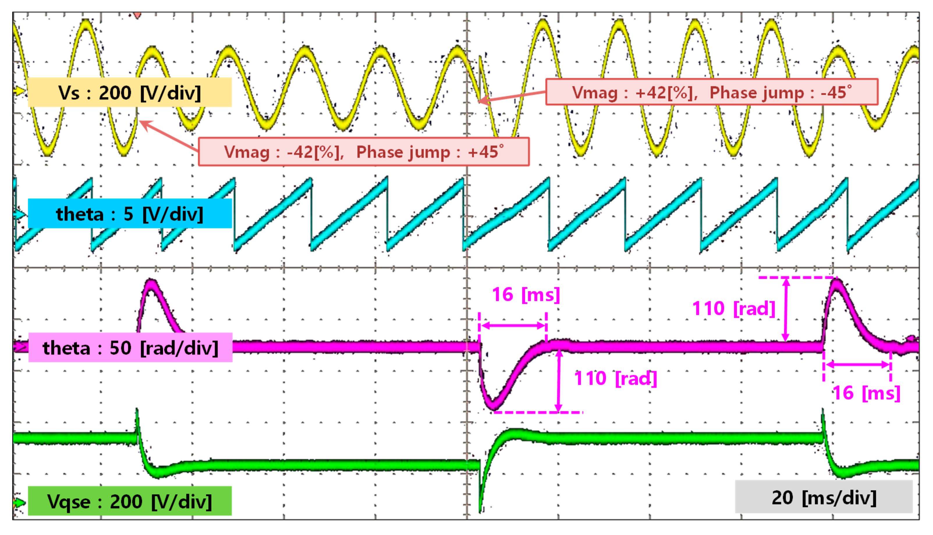
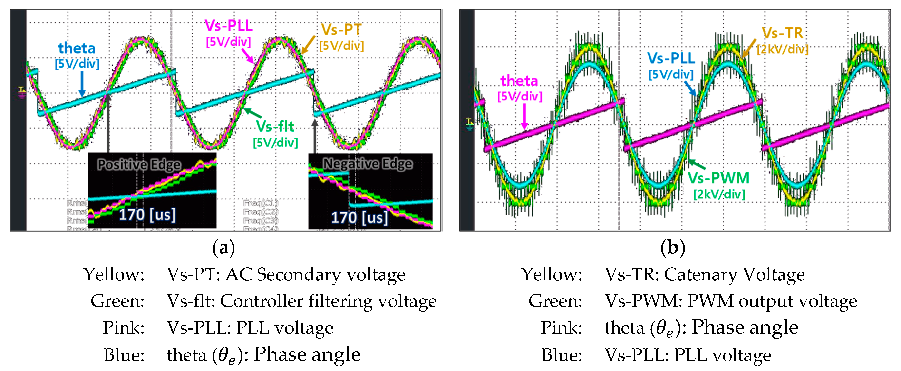
Figure 18 and Figure 19 show operating characteristics of the phase detection controller. The operating characteristics of the phase detector are described to verify the response characteristics of the PLL control at change amplitude and phase of the input voltage and to verify that the phase synchronization of the PCS output voltage is performed from the phase information detected by the PLL control.

Figure 18 shows the experimental results of the response characteristics of the PLL controller by applying a simulated signal to the input voltage sensor to change the amplitude and phase of the input voltage. From the experimental results, the response time was measured to be 16 ms and the overshoot angular frequency of line voltage was 110 rad, as shown in Figure 18, which were very similar to the simulation results shown in Figure 14.

Figure 19 shows that the PWM output voltage of the PCS detected from the actual catenary voltage is phase-synchronized through the phase information. Figure 19a also shows that the controller error according to the characteristics of the digital controller has one sampling error.

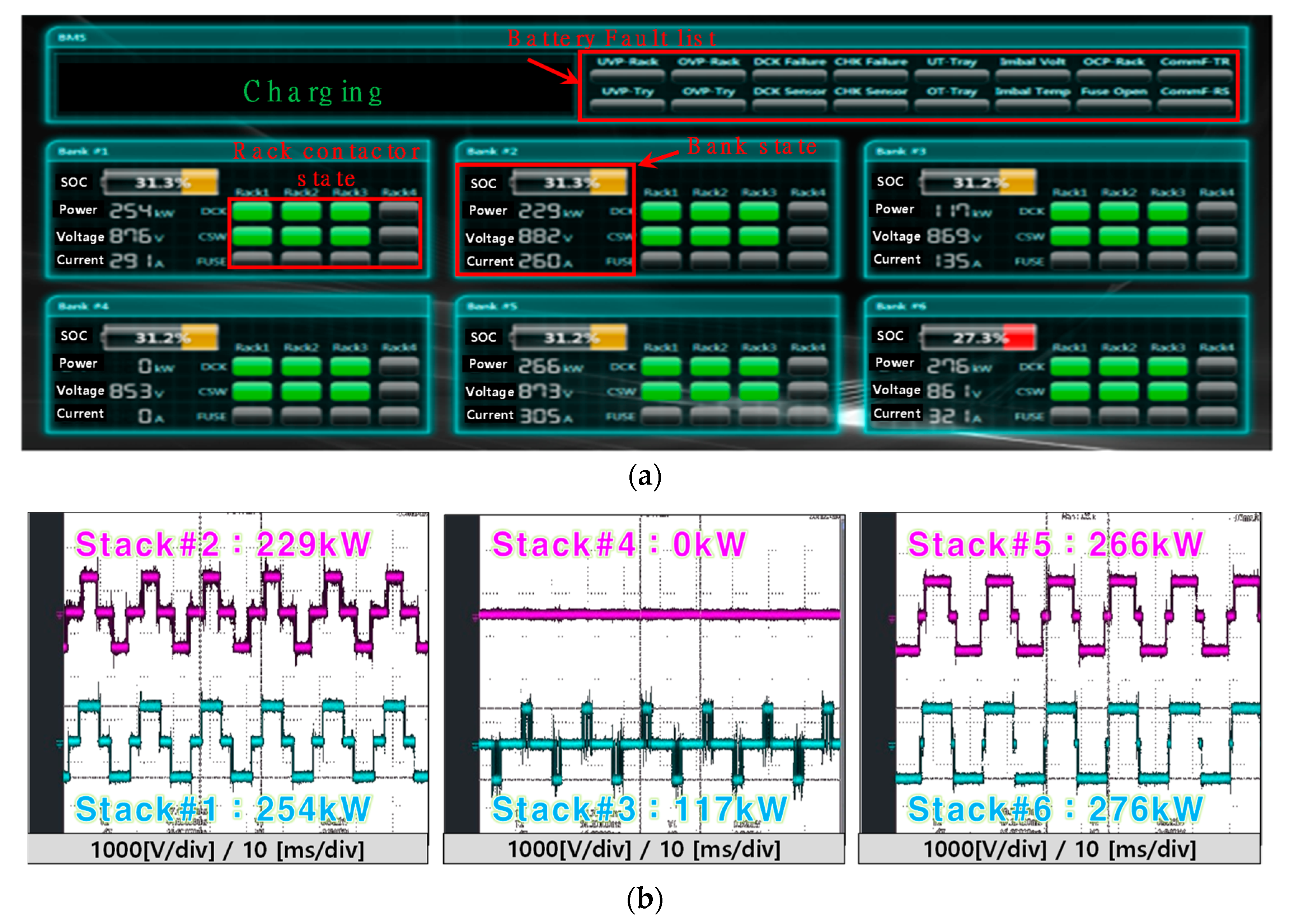
Figure 20 and Figure 21 show the operation of the battery balancing algorithm according to the operation state of the PCS and the SOC condition of the battery. To confirm the results of the experiment, PCS operation and battery status information were verified using the PMS. The output voltage of each cell inverter was measured using an oscilloscope. Figure 20a and Figure 21a show the results of checking the battery information on the PMS. Battery information is transmitted by communication from the system BMS to the PMS. The transmitted battery information displays the fault information of the battery and the operational status of each battery bank such as SOC, voltage, current, power, and rack contactor state.

Figure 20b and Figure 21b are output voltage waveforms of each cell inverter measured during PMS monitoring. The main measurement data in Figure 20 and Figure 21 are summarized, as shown in

Table 5. Battery and Cell Inverter Status Data by Mode in Figure 20 and Figure 21.

No.	RPR Mode: in the Case of Figure 20				ASS Mode: in the Case of Figure 21
	Battery Bank Voltage (V)	Battery Bank SOC (%)	Cell Inverter Power (kW)	Battery Bank voltage (V)	Battery Bank SOC (%)	Cell Inverter Power (kW)
1	884	46.7	166	876	31.3	254
2	882	46.3	167	882	31.3	229
3	890	46.7	167	869	31.2	117
4	886	46.6	166	853	31.2	0
5	889	46.3	166	873	31.2	266
6	882	46.3	164	861	27.3	276

.

As shown in Figure 20, the maximum deviation of the battery bank under RPR mode is 0.4%. Experimental results confirmed that the output of each cell inverter rotated at 100 ms cycles, as shown in the simulations, at which point, the power of each battery bank was charged equally at 166 kW. On the other hand, as shown in Figure 21, the maximum deviation of the battery bank under ASS mode is 4%. However, as shown in the experimental results, the power of each cell inverter is charging differently depending on the PCS condition and the SOC condition of each battery bank.

The change of the battery balancing mode is set through the hysteresis band. Changing mode by hysteresis band operates in the ASS mode when the battery bank SOC deviation is 5.0% or higher. It returns to the RPR mode when the battery bank SOC deviation is less than 2.0%. If the bandwidth of the hysteresis band is too narrow, the deviation in the battery bank will be smaller, making it possible to use the battery bank efficiently. However, it has the disadvantage of increasing the frequency of balancing mode transitions. On the other hand, if the bandwidth of the hysteresis band is too wide, it can reduce the frequency of balancing mode transitions. The drawback is that it is difficult to use battery banks efficiently.

Figure 22 shows output results when the PCS is operated from 500 kW to 2000 kW. The PCS power command is given by the inclination of 200 kW/s due to the power acceptability problems in tramway. The experimental results shown in Figure 22 are verification results of the waveform to the output voltage and current of the single-phase 13-level multi-level PCS for the power command. The output voltage and current of the PCS can be seen to be close to the sinusoidal waveform, as shown in the experimental results. In addition, the stable power to tramway is supplied without transient characteristics. It depends on the application of the slope in case of changed power command.

Table 6. Results of PMS Weekly Operational Data Analysis (KEPCO * I-Smart Interlink Analysis Data).

Target Peak Power: 24,000 (kW)
Date (month/day)	Without Peak Power Management (kW)	With Peak Power Management (kW)	Peak Power Savings (kW)	Peak Power Savings Rate
7/10	25,337	23,090	2247	8.87%
7/11	24,471	21,738	2733	11.2%
7/12	24,819	20,536	4283	17.3%
7/13	23,371	20,666	2705	11.6%
7/14	25,689	22,424	3265	12.7%
7/15	24,384	22,738	1646	6.75%

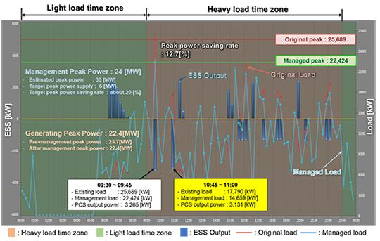
* KEPCO: Korea Electric Power Corporation.

shows operation data of PMS after applying the peak power reduction algorithm of the HSRS for a week. The PMS was configured to manage the peak power of the substation below 24 MW by using the 6 MW PCS with 2.68 MWh battery as in the simulation. As the experimental results show, the peak power was 23,090 kW on July 10 with the operation of the peak power reduction system. If the peak power reduction system was not operated, the peak power during that period might be 25,689 kW on July 14.

Figure 23 shows a detailed analysis of the PMS operation status data for July 14 from the operation data in Table 6. In Figure 23, the red solid line is the expected peak power when the peak reduction device is not activated, and the blue solid line is the actual generated peak power when the peak reduction device is operated. The blue bar represents the charge and discharge power of the peak reduction device.

These experimental results confirmed that the PMS accurately estimated that the peak power was generated at 09:30 AM. At this point, the PCS also supplied 3265 kW of power to the tramway by the PMS command, thereby managing the peak power at 22,424 kW.

If the peak power of the substation is 30 MW within the operating period of the demo system, it is expected that PPRS would have reduced the peak power of the substation to 24 MW by supplying 6 MW to the tramway. This is about a 20% reduction in peak power for substations [37].

6. Conclusions

This paper proposed the single-phase 13-level PCS for peak power reduction of HSRS. The GRG optimization algorithm was applied to the PMS for the management of peak power. The PCS is the configuration of a single-phase 3100 V, 2 MVA, 13-level H-bridge multi-level inverter, which has excellent power quality. In addition, it is easy to serialize by voltage. Moreover, the DC bus power of each cell inverter was supplied by lithium-ion batteries. The phase detector and power controller for the control of a single-phase PCS based on the virtually coordinated axes using an all-pass filter were proposed to be robust to external disturbances with fast response characteristics. This study also proposed the ASS method, which changes the switching depending on the operation state of PCS and the SOC of the battery to minimize battery imbalance by controlling each cell inverter of the H-bridge.

The validity of the proposed system was verified by PSiM simulation and experiments. Especially, the experiment was run for a week with a 6 MW PCS and 2.68 MWh batteries as a demo system at one HSRS of KORAIL under commercial operation. As the results of the operation showed, the PMS accurately predicted the peak power generation time of the substation and managed the peak power of the substation within the target peak value of 24,000 kW. The proposed PCS was supplied accurately from the PMS power command through the phase detection controller and the power controller. In case of voltage deviation of each battery bank, the RPR mode and ASS mode were automatically switched by the battery voltage balancing controller to control the voltage. Therefore, each battery bank could use the SOC from 5% to 95% practically. In the future, it is necessary to continuously obtain operation data to ensure the reliability and stability of the performance and operation of the proposed system.