Article

Dynamic Impedance of the Wide-Shallow Bucket Foundation for Offshore Wind Turbine Using Coupled Finite–Infinite Element Method

1
State Key Laboratory of Hydraulic Engineering Simulation and Safety, Tianjin University, Tianjin 300350, China
2
School of Civil Engineering, Tianjin University, Tianjin 300350, China
3
Power China Huadong Engineering Corporation Limited, No.201 Gaojiao Road, Yuhang District, Hangzhou 311122, China
*
Author to whom correspondence should be addressed.
Energies 2019, 12(22), 4370; https://doi.org/10.3390/en12224370
Submission received: 27 September 2019 / Revised: 29 October 2019 / Accepted: 14 November 2019 / Published: 16 November 2019
(This article belongs to the Special Issue Foundation Systems for Offshore Wind Turbines)

Abstract

:
The dynamic impedances of foundation play an important role in the dynamic behavior and structural stability of offshore wind turbines (OWT). Though the behaviors of bucket foundation, which are considered as a relatively innovative foundation type under static loading, have been extensively investigated, the corresponding dynamic performances were neglected in previous research. This study focuses on the dynamic impedances of wide-shallow bucket foundations (WSBF) under the horizontal and rocking loads. Firstly, the numerical model was established to obtain the dynamic impedances of WSBF using the coupled finite-infinite element technique (FE-IFE). The crucial parameters affecting the dynamic responses of WSBF are investigated. It is shown that the skirt length mainly affects the rocking dynamic impedance and the diameter significantly affects the horizontal and coupling impedances, especially when the diameter is larger than 34 m. The overall dynamic responses of WSBF are profoundly affected by the relative soil thickness and the multi-layer soil stiffness. Additionally, dynamic impedances of WSBF are insensitive to the homogeneous soil stiffness. Lastly, the safety threshold curve was calculated according to the OWT, which can provide essential reference for the design of the OWT supported by large scale WSBF.

Graphical Abstract

1. Introduction

Currently, bucket foundation has been put forward as an innovative foundation type which is applicable to softer soil conditions due to its cost-effectiveness and high-reliability [1,2] compared with the other various foundation types [3,4,5], including monopile [6,7], concrete pile-supported square footing [8], gravity, tripod [9], jacket [9,10], and floating [11], which were designed for different environmental and geological conditions. The bucket foundation normally consists of skirt and lid, which constitutes an upside-down bucket [12] and may be used as an offshore wind turbine foundation in appropriate soil conditions [13,14]. The most outstanding advantages of this foundation type are high lateral and moment resistance, which are provided by the extended cylindrical skirt and compartments [15]. In the installation process, the bucket foundation is firstly penetrated into the seabed by its self-weight and then by the suction or pumping devices without the installation equipment as lifting and heavy punch machines [16]. Hence, the application of this novel foundation will greatly save high installation costs as well as construction time. According to the slenderness ratio (depth to diameter ratio), the bucket foundations can be divided into two types, namely, narrow deep and wide shallow [15]. In project engineering, the wide-shallow bucket foundations (WSBF) have been applied in offshore wind farms (OWF) including Frederikshavn, Denmark, 2002 [17], Qidong, China, 2010 [18], and Xiangshui, China, 2017 [19], respectively, as shown in Figure 1.
It is widely recognized that the design of the OWT requires accurate evaluations of the natural frequency and dynamic response, which are dependent on the dynamic impedance of the foundation and soil-foundation interaction. In previous studies, several analytical and numerical methods have been applied to evaluate the dynamic responses of an embedded foundation for OWT structures within the elastic half-space under idealized conditions. The dynamic impedances of end bearing piles, floating piles and suction caissons shown in Figure 2 were studied. Wolf et al. [20,21] provided an analytical and semi-analytical solution for foundation vibration including end bearing pile and suction foundation employing cone model based on strength of materials (Figure 2a). A new polynomial representation of impedance function based on Winkler model for equivalent-linear characterization of the pile is proposed by Torabi et al. [22], especially in the rock-socketed piles. Harte [23] considered the foundation of a wind turbine as a rigid gravity based foundation which is connected to the surrounding soil to obtain complex impedance using cone model, and investigated the influences of the interaction between the foundation and the soil on the dynamic response. Latini et al. [24,25,26] studied the dynamic performances of floating piles and suction caissons (Figure 2b,c) by a three-dimensional finite element model in frequency domain, exploring groups of dimensionless parameters related to the soil and foundation and their effects on the dynamic response of foundation considered. Gerolymos et al. [27,28] developed Winkler model to calculate the static and dynamic responses of caisson foundations (Figure 2c) accounting for nonlinear interface through spring and dashpot, and this nonlinear Winkler-spring method was implemented in a new finite difference time-domain code, NL-CAISSON [29]. Damgaard et al. [30,31] inserted a standard lumped-parameter model into the aeroelastic code FLEX5 to consider the dynamic interaction between the foundations and subsoil, which could be used to calculate the dynamic vibration response of OWT. Andersen et al. [32] established the lumped-parameter models as well as a coupled finite-element/boundary element scheme to analyze the bucket foundation of OWT in both time and frequency domains. An improved lumped-parameter model of foundation based on complex Chebyshev polynomials was proposed by Wang Hai et al. [33], which can reduce the unexpected wiggling in the foundation model, improve the accuracy, and needs fewer parameters. Liingaard [34,35] presented a three-dimensional coupled boundary element/finite element model and lumped-parameter models to indicate the frequency dependent impedance of the rigid and flexible bucket foundation (Figure 2c) for the OWT. He et al. [36,37] modeled the bucket foundation as a rigid cylindrical shell embedded in a homogeneous sandy seabed to obtain the vertical and lateral dynamic impedance of the bucket foundation by the Green’s function and boundary conditions (Figure 2c). Doherty et al. [38] applied the scaled boundary finite element method to obtain the stiffness coefficients, which can represent the dynamic behavior of a bucket foundation in the elastic regime. Ba et al. [39] proposed an indirect boundary element method to obtain the dynamic impedance of a surface rigid strip footing resting on the multi-layered transversely isotropic saturated half-space. Jalbi et al. [10] made use of extensive finite element analysis by PLAXIS 3D to derive closed form expressions for dynamic lateral, rotational, and cross-coupling impedance of rigid skirt caissons. Combined with the characteristics of the suction caissons, dynamic impedance functions were proposed in the previous pieces of literature based on the Winkler model, lumped-parameter model, and the evaluation accuracy of those functions was improved by using different finite element methods.
As described in Figure 2, the geometry of WSBF is different from the previous pile and narrow-depth bucket foundations because of the large diameter and a relatively small length skirt. Moreover, the WSBF is top bearing capacity, and the rotation is the main failure model, which are completely different from traditional suction caissons [40]. Furthermore, the current codes of practice, including DNV(Det Norske Veritas) [41] and IEC(International Electrotechnical Commission) [42], for the design of OWT structures have no clear calculation method on the dynamic impedance and stiffness characteristic of the WSBF. The main reason may be that the WSBF has not been widely used for OWF around the world and lacks comprehensive investigation or long-term monitoring. Therefore, it is urgent to explore the dynamic impedance of the WSBF to understand the interaction mechanism between the foundation and soil.
Different from previous research, this study is to carry out the dynamic impedance characteristics of the WSBF for OWT through the coupled finite-infinite element technique (FE-IFE). The frame of this paper is organized as follows: Firstly, the methodology concerning the dynamic impedance, the coupled FE-IFE technique, and its implementation in the numerical model are introduced in Section 2. Secondly, the dynamic impedances of WSBF are obtained by performing steady state dynamic response analysis subjected to harmonic excitation in the frequency domain. The influencing parameters on the dynamic impedances are discussed based on a numerical example in Section 3. Section 4 discusses the influences of various dimensionless parameters on structural dynamic impedances. Further, taking one offshore wind farm as an example, the safety threshold envelope of the WSBF geometry dimension is calculated according to the FE-IFE technique in Section 5. Lastly, the conclusions of the whole work and the outlook for further studies are both illustrated in Section 6.

2. Methodologies

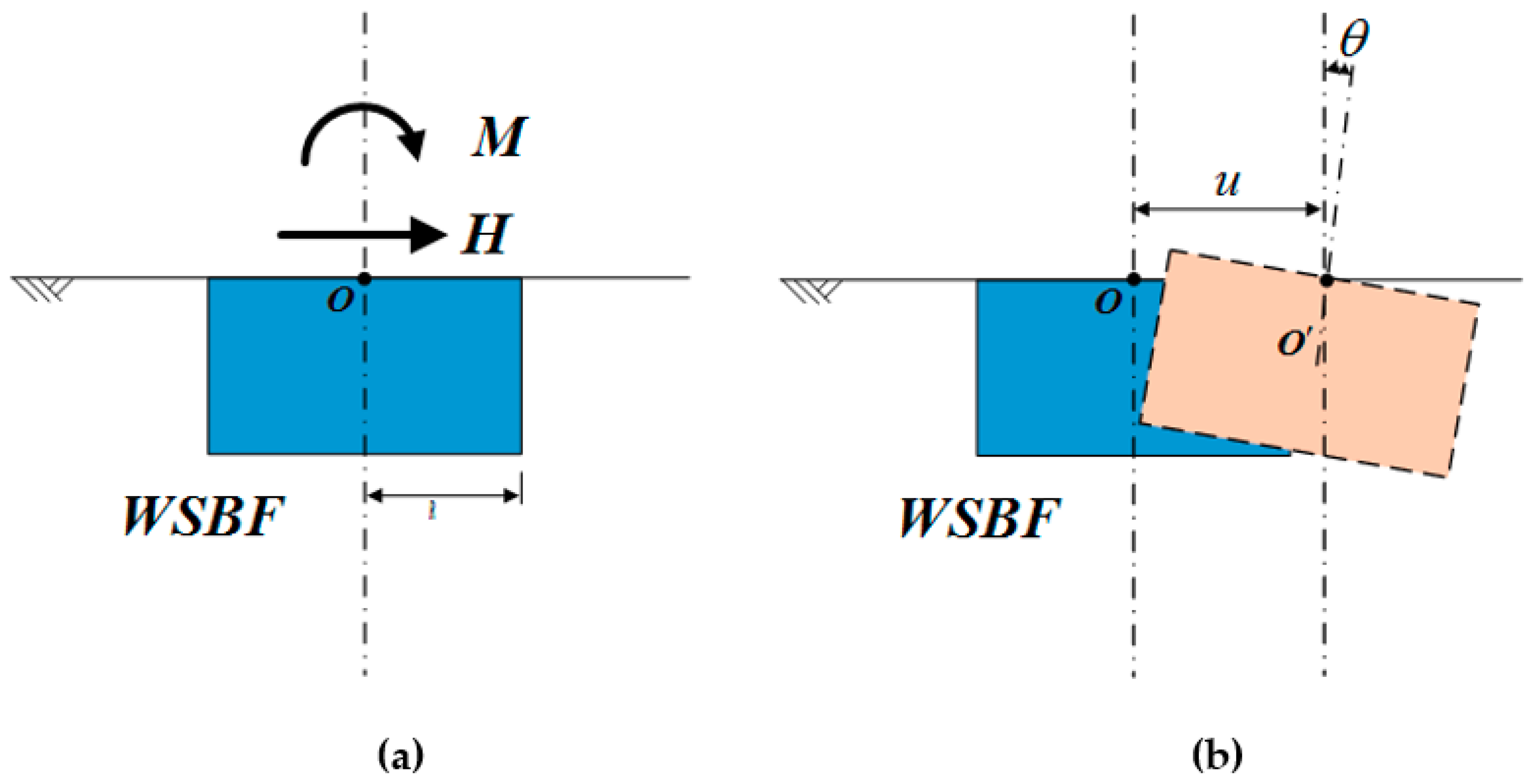
2.1. Dynamic Impedance of the Wide-Shallow Bucket Foundations (WSBF)

The motion of the WSBF can be simplified and described as a rigid foundation under the assumption that the structure is so much stiffer than the surrounding soil that the deformation of WSBF can be negligible. Therefore, the in-plane degrees of freedom for a rigid WSBF including displacement, and rotation, and the corresponding force and moment are illustrated in Figure 3. If the dynamic impedances of the WSBF are evaluated in the frequency domain, the dynamic behavior of the foundation can be described by the dynamic-impedance matrix as follows [32]:
F ( ω ) = K ( ω ) Z ( ω )
where ω is the harmonic frequency, F , K , Z are force or moment vectors in complex frequency domain, dynamic impedance matrix, and vector of displacements or rotations in complex frequency domain, respectively.
According to Figure 3, the head of the WSBF subjected to lateral unit dynamic excitation H and M, combined with Equation (1), the component form of WSBF can be written as [32]:
[ H / G s R 2 M / G s R 3 ] = [ K h h K h r K r h K r r ] [ u / R θ / R ]
where Gs is the shear modulus of the soil, u and θ are the displacement and rotation angle of the WBSF, respectively, and R is the radius of the WSBF. K h h , K r r and K r h ( K h r ) represent the dynamic impedance in horizontal, rocking, and coupling, respectively. The coupling terms, K r h and K h r assumed to be equal, because a symmetric stiffness is expected.

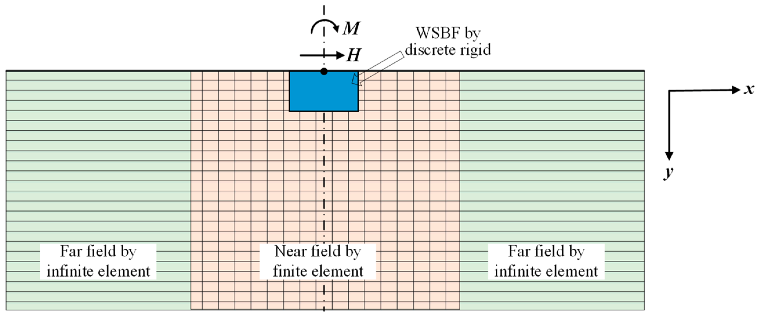
2.2. Coupling Finite-Infinite Element (FE-IFE) Technique

When the numerical model of WSBF is embedded in a bounded domain, the phenomenon of spurious reflection wave induced by the truncated boundary deserves more attention, especially under the high frequency excitation conditions. To solve this problem, a new simulation method called the FM-IFEM technique [43,44,45] was introduced to calculate the dynamic behaviors of WSBF in this study.
The two-dimensional WSBF model embedded in an elastic half-space can be described in Figure 4. In the numerical model, the near field and far field regions will be analyzed through the finite element and infinite element methods, respectively.
Considering the external load F ( x , y ) exp ( i ω t ) , the displacement field of the system can be expressed as follows [44]:
u ( x , y , t ) = u ^ ( x , y ) exp ( i ω t )
where u ^ ( x , y ) denotes the displacement field of the two-dimension field and t is the time.
Based on the finite element procedure, the displacement u ^ ( x , y ) of each element in the near field domain can be interpolated as follows [43]:
u ^ ( x , y ) = i = 1 n N i u i
where N i is the displacement shape function, i is the node order and n is the number of nodes for each element. The coordinates x and y within the element can be expressed as [43]:
x = i = 1 n M i x i ,   y = i = 1 n M i y i
where M i is the shape function for both displacement and the coordinate for the node i. Substituting the displacement field in Equation (3) into the equation of virtual work and performing the Galerkin weighted residual procedure, the equation of motion in frequency domain can be written as [43]:
( [ K ] + i ω [ C ] ω 2 [ M ] ) { D } = { F }
where { F } and { D } denote the vector of external load and the vector of nodal displacement, respectively, and i is the imaginary unit. [ K ] , [ M ] and [ C ] are the global stiffness, mass, and damping matrices of the system, respectively.
The concept of infinite elements was first proposed by Ungless and Bettess. Since the concept of infinite elements is essentially the same as the finite elements except for their shape functions, Equation (6) is applicable to both finite and infinite elements. In the infinite elements method, to ensure the accuracy of the result needs the shape function, which is known as the ‘decay function’ in the static problems and ‘wave propagation function’ in the dynamic problems. According to the propagation direction in the infinite region, there are three types of infinite elements, which are used to simulate wave propagation along with the horizontal, vertical and both horizontal and vertical directions.
The first kind of infinite element (IE1) is to simulate the wave propagation along horizontal direction. The horizontal shape function is built based on the dynamic solution of homogeneous elastic half-space and can be written as [44]:
N u x , i = F u x ( ξ ) φ i
N u y , i = F u y ( ξ ) φ i
in which:
F u x ( ξ ) = J 1 ( κ ( x 0 + ξ ) ) J 1 ( κ x 0 ) = H 1
F u y ( ξ ) = J 0 ( κ ( x 0 + ξ ) ) J 0 ( κ x 0 ) = H 2
where J 0 ( x ) and J 1 ( x 1 ) represent the Bessel function of the first kind of zero and the first order, respectively. κ is wavenumber, x 0 denotes the horizontal distance between the origin of the coordinate system and the starting point of the IE1. φ 1 , φ 2 and φ 3 are the standard shape functions in the η direction and expressed as following [44]:
φ 1 = 1 2 η ( η 1 )
φ 2 = 1 η 2
φ 3 = 1 2 η ( η + 1 )
The second kind of infinite element (IE2) is to simulate the wave propagation along vertical direction. The shape function can be expressed as following [44]:
N u x , i = N u y , i = e χ η φ i
where χ = ( ε / λ P 1 ) + i ( ω / V P 1 ) in which λ P 1 and V P 1 denote the wavelength and velocity of the first P wave, respectively. ε is an experimental coefficient. φ 1 , φ 2 and φ 3 are the standard shape functions in the ξ direction and defined as following [44]:
φ 1 = 1 2 ξ ( ξ 1 )
φ 2 = 1 ξ 2
φ 3 = 1 2 ξ ( ξ + 1 )
The third kind of infinite element (IE3) is to simulate the wave propagation along both vertical and horizontal directions. Combination with the above two infinite elements, the displacements of the third kind can be defined as [44]:
u x ( x , y , t ) = e χ ( y y 0 ) H 1 u x 1
u y ( x , y , t ) = e χ ( y y 0 ) H 2 u y 1
where y 0 is the vertical distance between the origin of coordinate and starting point of IE3, u x 1 and u y 1 are the displacements of node 1 for IE3. For more detailed FE-IFE technique refer to reference [44].

2.3. Steady-State Dynamic Analysis

According to the theory of dynamic impedance, the 3D finite-infinite element model was applied to analyze the dynamic impedance of WSBF, which is considered as a rigid body, embedded in a soil layer on bedrock. The center of the foundation head is subjected to the harmonic load or harmonic bending moment P = P 0 e i ω t , which generates harmonic oscillations of the form U = U 0 e i ( ω t φ ) . ω represents the cyclic excitation frequency and φ describes the phase difference between horizontal vibration of WSBF and excitation force.
In the calculation of steady state linear dynamic analysis, the dynamic impedance of the WSBF is defined as the ratio between the unit harmonic force acting on the foundation and its vibration response amplitude, which is a frequency dependent complex-valued and its equation is shown as following [37,38]:
K ( ω ) = K M ω 2 + i ω C = P ( t ) U ( t ) = P 0 e i ω t U 0 e i ( ω t φ ) = P 0 U 0 cos φ m ω 2 + i P 0 U 0 sin φ
The investigated excitation frequency ranges from 0 Hz to 10 Hz, i.e., dimensionless excitation frequency ranges from 0 to 5, as the external loads acting on the offshore wind turbine belong to lower frequency during the operating condition. The stiffness range considered in this paper is from 1 × 10⁸ to 1 × 10¹¹ while the value of inertial term is 1 × 10⁷, so the value of m ω 2 is relatively small comparing with stiffness. It is reasonable to neglect its influence on the dynamic stiffness coefficients. Then the initial dynamic impedance of WSBF is expressed as follows [37,38]:
K ( ω ) = P 0 U 0 cos φ + i P 0 U 0 sin φ
where P 0 and U 0 are the magnitude of the excitation response and displacement of foundation, respectively.
The real part of K ( ω ) represents the dynamic stiffness of WSBF and the imaginary part denotes the dynamic damping of the WSBF shown as follows [37,38].
K = Re ( K ( ω ) ) = P 0 U 0 cos φ
C = Im ( K ( ω ) ) = P 0 ω U 0 sin φ
where, the K and C are the dynamic stiffness and dynamic damping of WSBF, respectively.

3. Numerical Examples

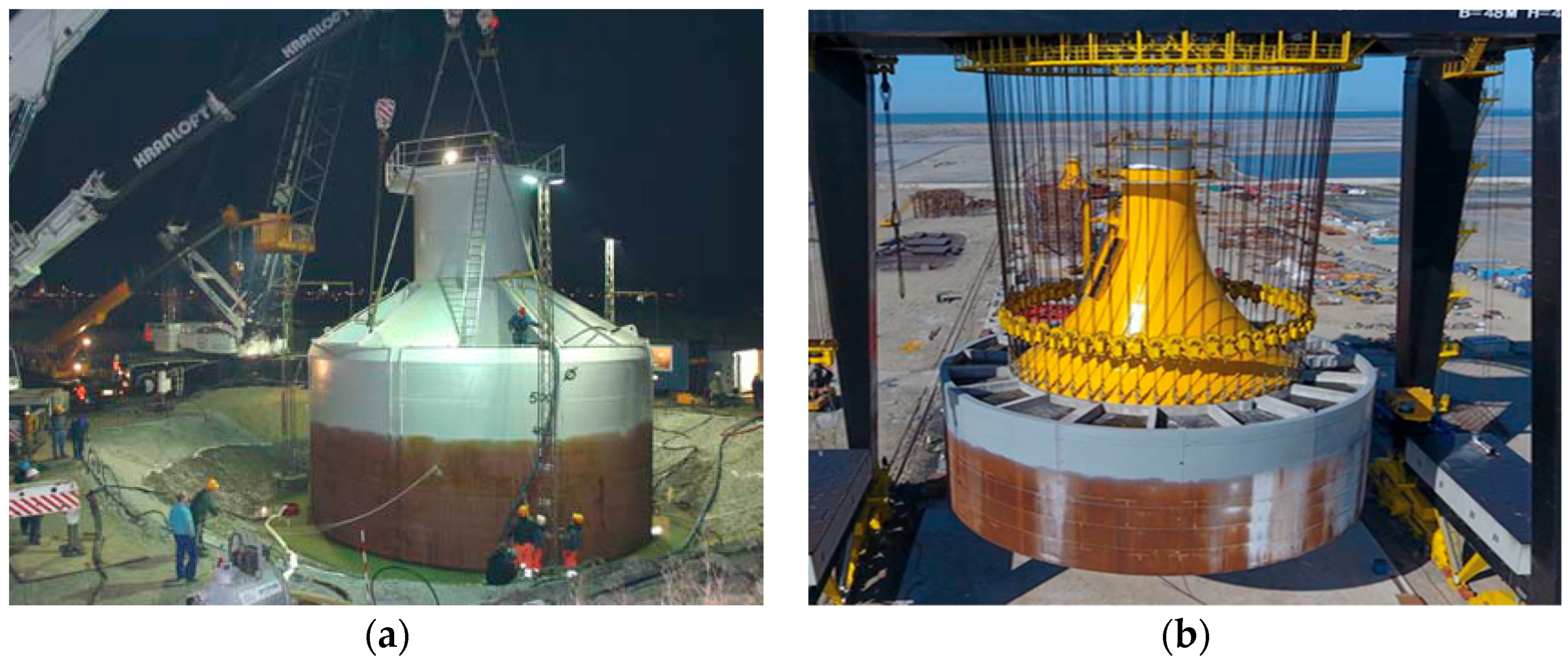
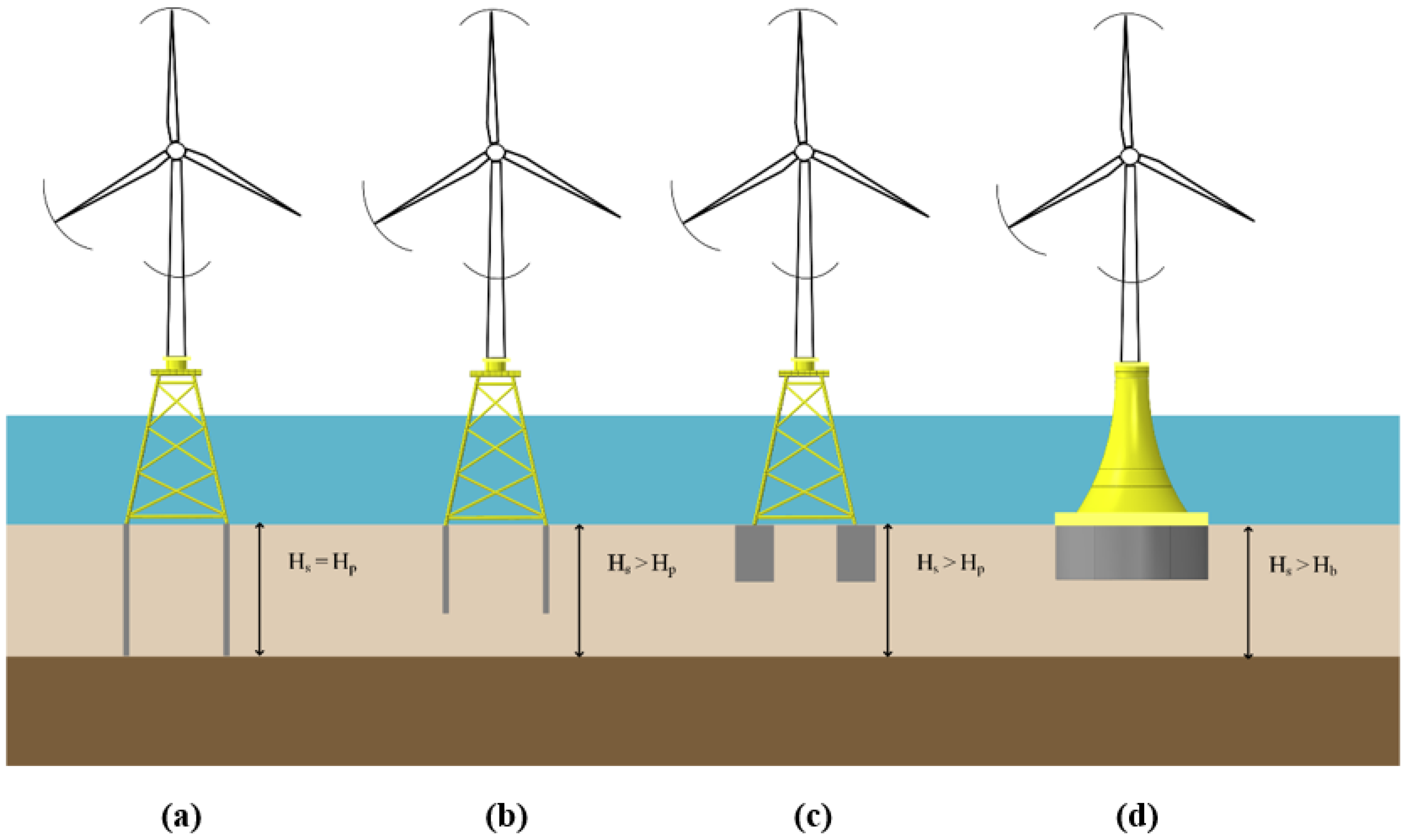
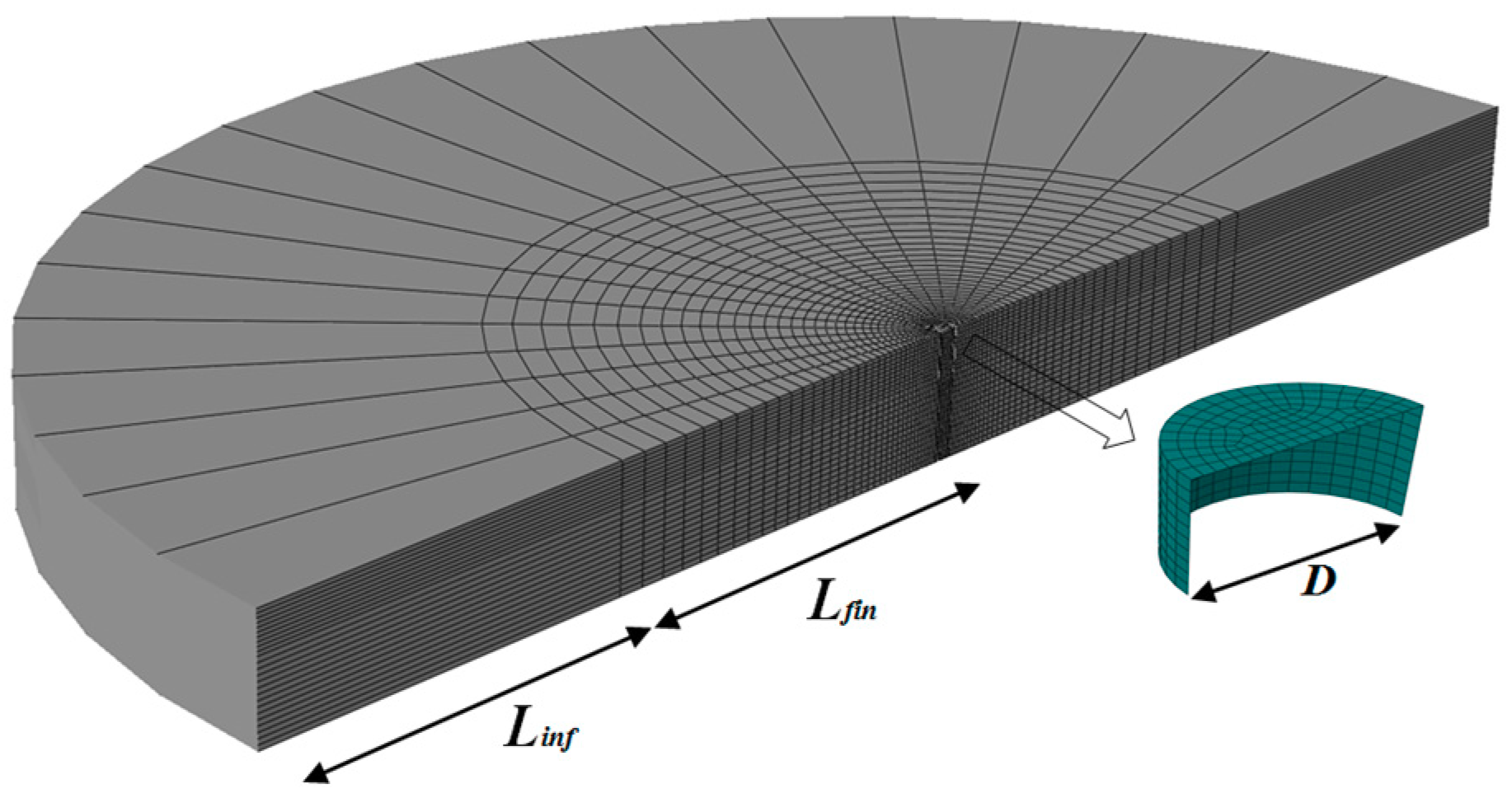
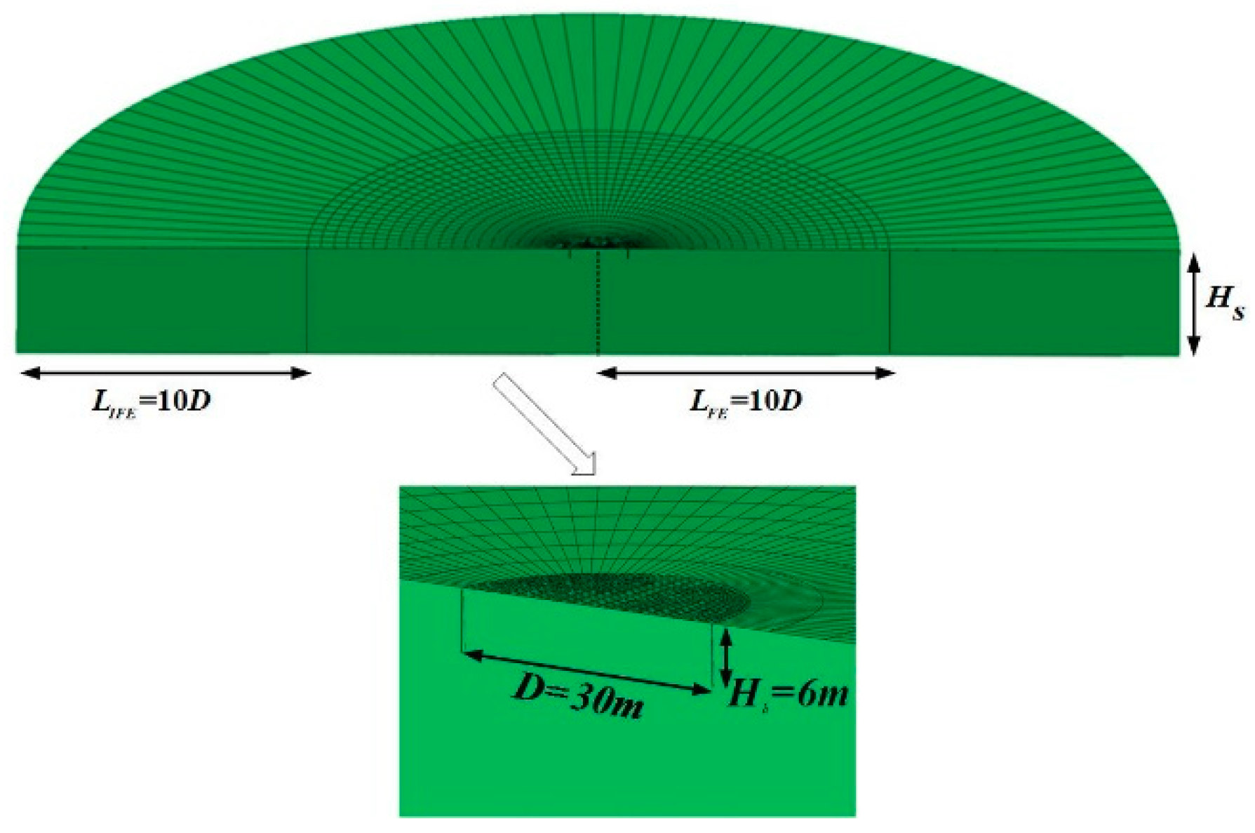
3.1. Numerical Model

Modeling considerations—to better understand the dynamic impedances of the WSBF, a series of three-dimensional FE-IFE models were constructed to analyze the dynamic responses. As mentioned in references [26], three hypotheses should be clarified in the numerical model: (1) The rigid WSBF, (2) constant damping ratio of soil, (3) perfect bonding at the soil-foundation interface during the analysis.
Due to the symmetry of the model, only half of the foundation and surrounding soil was taken into consideration in the numerical models as shown in Figure 5. Two different modelling approaches were used: (1) Shell element, where the WSBF was modeled by shell elements (S4); and (2) equivalent solid element, where the soil was discretized by solid elements to match the bending stiffness of the WSBF and the inner soil. The far field soil was modeled using infinite elements (CIN3D8) in order to avoid the spurious reflections, while the near field soil domain was discretized by 8-node 3D continuum elements (C3D8R). The foundation surface and surrounding soil were bonded together to satisfy displacement compatibility to avoid the nonlinear interface. Next, the steady-state dynamics response of the models subjected to harmonic excitation in the frequency domain was calculated.
Element sizes—to accurately simulate the wave propagation in the elastic soil, the mesh size was set small enough to capture the stress waves even at high frequency range. Hence, the maximum of the size of the elements size should meet the following requirement [46]:
l max ( 1 8 ~ 1 5 ) 2 π R a
where a = ω R / c s is the dimensionless frequency, ω , R and c s are respectively the frequency, the foundation radius, and the shear wave velocity of the soil.
Moreover, in order to minimize the error induced by numerical shock and coupling boundaries, the requirement of the near field domain modeled by the finite element can be expressed as:
l r 2 m π R a 2 2 v 1 2 v
where l r represents the minimum reflection length of finite element. m is the cycle number of excitations. v is Poisson’s ratio of the surrounding soil.

3.2. FE-IFE Model

Based on practical engineering, the typical WSBF was selected to illustrate the dynamic response of the foundation. The FE-IFE model of WSBF is shown in Figure 6. In the present analysis, the material properties of the soil and the foundation were identified by the subscripts s and b. The WSBF consists of steel with diameter D = 30 m, skirt length Hb = 6 m, Young’s modulus Eb = 210 GPa, and Poisson’s ratio νb = 0.3. The foundation head thickness tlid and foundation skirt thickness tskirt are 10 mm and 20 mm, respectively. The thickness of the soil layer is Hs = 60 m, with the density of 1800 kg/m3 and Poisson’s ratio of 0.38. The soil surrounding foundation has viscous damping of 5% and modulus of elasticity Es = 6 MPa. According to the Section 3.1, the near soil filed domain (Lfin = 10 D) was described by the hexahedral elements and infinite elements (CIN3D8) are placed at the far filed soil to avoid the spurious reflection.
By applying a static horizontal unit displacement on the top of the WSBF, the static stiffness terms K h h 0 and K h r 0 can be obtained. Similarly, the static stiffness terms K r r 0 and K h r 0 can be obtained by imposing a unit rotation on the top of the WSBF with zero horizontal displacement. K h h 0 and K h r 0 represent the static horizontal stiffness and static coupling stiffness, respectively. K r r 0 represents the static rocking stiffness.
The steady-state linear response of the model is performed to obtain the dynamic impedances ( K ( ω ) ) of the WSBF using the frequency-domain method. At the same time the first eigenfrequency f1 of foundation was calculated as 4.73 Hz. The dynamic impedance variation of WSBF with the change of excitation frequency is displayed in Figure 7. A dimensionless frequency related to the eigenfrequency of WSBF is introduced to analyze the dynamic response of foundation conveniently.
α 0 = ω / 2 f 1
where f1 is first eigenfrequency of foundation.
In Figure 7a,c,e, the ordinates are the normalized coefficients of the three types of dynamic stiffness ( K h h , K h r , K r r ) divided by the corresponding static stiffness ( K h h 0 , K h r 0 , K r r 0 ), which represent the dynamic stiffness amplitude factor in horizontal, coupling, and rocking directions. In Figure 7b,d,f, the ordinate state normalized magnitudes of the dynamic damping divided ( C h h , C h r , C r r ) by the dynamic stiffness, which represents the dynamic damping ratio of the soil-foundation system.
As described in Figure 7a,c,e, the three kinds of normalized magnitudes of dynamic stiffness including horizontal stiffness (Khh), rocking stiffness (Krr), and coupling stiffness (Khr) show an obvious decreasing trend before the first eigenfrequency because of the constant static stiffness value. Only one drop in stiffness line can be found at the first eigenfrequency of bucket foundation, along with the minimum value of the dynamic stiffness, due to the resonance effect. Subsequently, the horizontal stiffness and coupling stiffness coefficients are characterized by an increasing slope linearly with excitation frequency. In general, the overall dynamic stiffness coefficients first reach minimum values and then increase linearly, when the dimensionless frequency is between 3.0 and 3.5 (3.0 < α0 < 3.5). Within the higher frequency range (larger than α0 > 4), the dynamic stiffness coefficient increasing values exceed the static stiffness. It can be explained that the dynamic stiffness still keeps sensitive in the change of excitation frequency; on the contrary, these frequencies which are gradually far away from the first eigenfrequency of foundation also make the structural dynamic responses weaker. Differently, the rocking stiffness coefficient firstly rises and then decreases linearly with the increase of the excitation frequency after the first eigenfrequency.
The variation trends of dynamic damping with the change of excitation frequency are described in Figure 7b,d,f. It appears that the overall damping coefficients express an increasing trend and reach the peak value at the first eigenfrequency. After the first natural frequency of WSBF, all the damping firstly decreases and then rises exponentially with the increase of excitation frequency.

4. Parametric Study

The dynamic responses of the foundation are influenced by many factors. In order to determine the dominant sensitive factors on the dynamic responses of WSBF, the key parameters such as the slenderness ratio, the skirt thickness, the soil layer thickness, the stiffness of homogeneous soil and multi-layer soil were explored. A series of numerical models with the above crucial parameters related to foundation geometry and soil were constructed. The cases and the corresponding parameters are listed in Table 1.
The shear modulus varies with the depth below ground surface in the practical engineering. Gibson model was adopted to simulate the actual stiffness variation of soil to evaluate accurately the dynamic impedances of WSBF. In that model, it is an assumption that the elastic modulus of the soil layer is taken to have a power law variation with the depth according to the following expression [47]:
G ( z ) = G 0 + ( z R ) b
where z is the depth from the ground surface, G 0 represents the reference shear modulus at a depth equal to the radius of the foundation (R) and b is a dimensionless inhomogeneity factor that varies between 0 and 1.
In this paper, three different soil profiles are considered. The profiles with different elastic modulus distribution are indicated in Figure 8. Profile A shows a fixed elastic modulus, i.e., homogeneous soil layer, and the parameter b is set as zero. The value of the parameter b of Profile B is 1, which represents the normally consolidated clay. Profile C depicts the normally consolidated sand where the parameter b is set as 0.5. The viscous damping coefficient of the soil layer is 5% and Poisson’s ratio is 0.38 for all the cases in Table 1. These three soil profiles may sufficiently represent the characteristics of a wide range of real soil profiles.
According to the established WSBF and integrated transportation requirements, the diameter of foundation selected in the numerical analysis varies from 30 m to 45 m (cases 3,5–7), and the skirt length from 3 m to 20 m (cases 1–4) based on the water depth. The thickness of the shirt differs from 20 mm to 50 mm due to construction procedure restriction (cases 3,11–13). The elastic modulus of soil property belonging to silt and silty clay varies from 6 MPa to 24 MPa (cases 3,14–16).

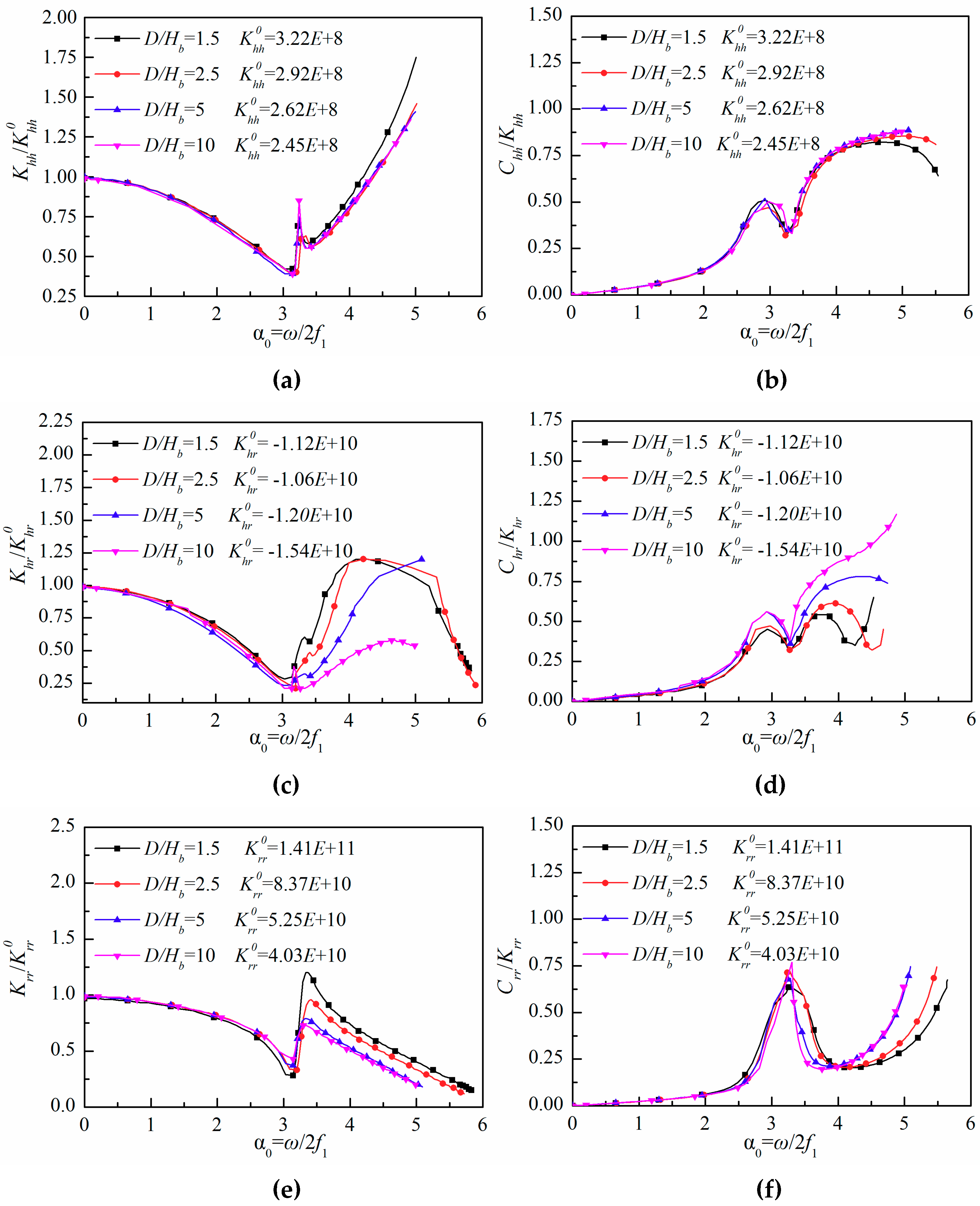
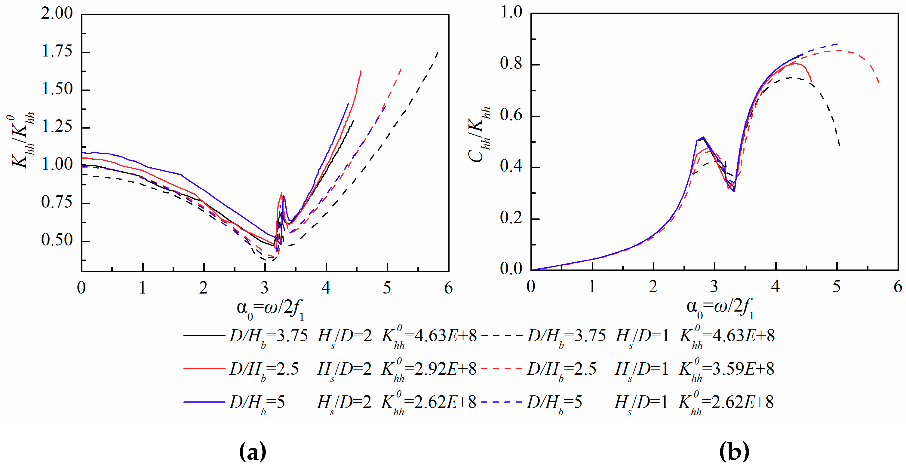
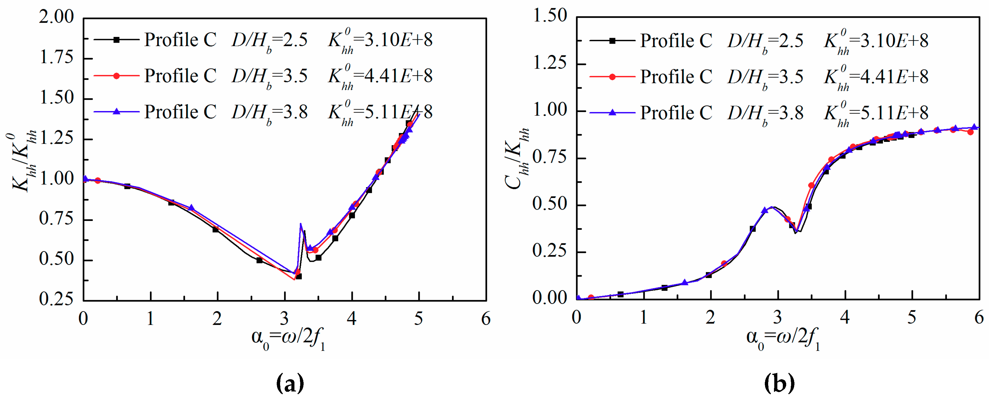
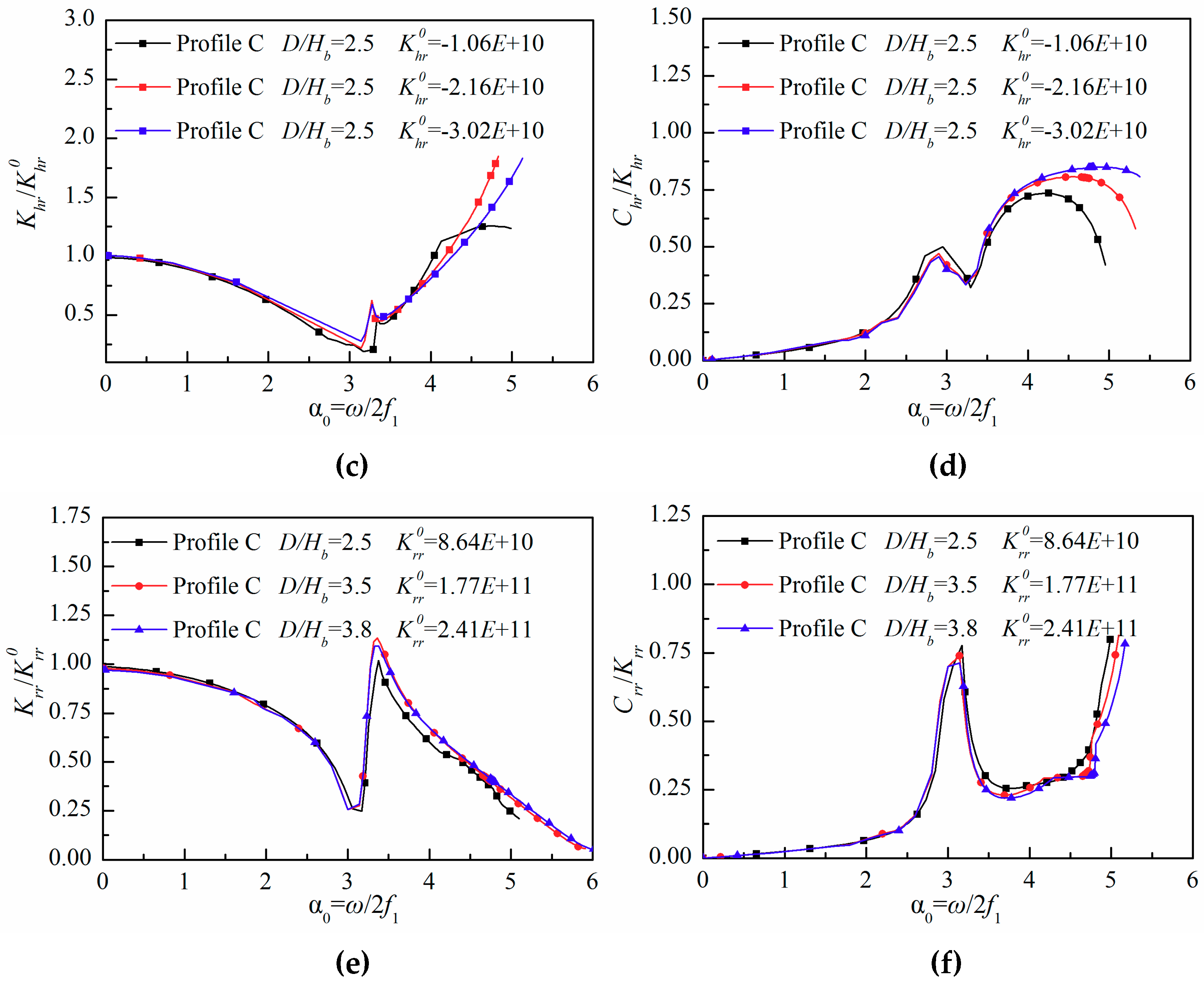
4.1. Influence of Slenderness Ratio

The trends of dynamic stiffness and damping coefficients with dimensionless excitation frequency under different slenderness ratio by varying the skirt length are depicted in Figure 9 (cases 1–4, listed in Table 1). It appears that the overall dynamic stiffness and damping coefficients vary with the excitation frequency. After the first eigenfrequency, they are affected by the slenderness ratio because of the different skirt length. While, before the first eigenfrequency, they have the same trend. The dynamic stiffness coefficients variation with excitation frequency are affected slightly by the slenderness ratio when the frequency exceeds the first eigenfrequency. It can be seen that the horizontal dynamic stiffness coefficients grow sharply in the higher frequency range (larger than α0 > 4) with the decrease of the slenderness ratio. The coupling and rocking stiffness coefficients seem to be profoundly affected by the slenderness ratio. The coupling stiffness coefficient gradually reaches peak against the slenderness ratio and decreases subsequently with the increase of excitation frequency. For the rocking stiffness coefficient, it is observed that the increase of slenderness ratio would result in lower decrease slope. It is clear from the variation of dynamic stiffness coefficients that with more rotation and less horizontal control the dynamic responses, along with the skirt length, increase.
The damping coefficients under the influence of slenderness ratio caused by varying the skirt length keeps consistent with the dynamic stiffness, which appears insensitive to the slenderness ratio at a lower excitation frequency range. Regarding the higher frequency range (larger than α0 > 3.2), distinctively different behavior of coupling damping coefficient is observed for slenderness ratio lower than 4, where the increase in the damping became less marked as the slenderness ratio decreased and reached the peak and trough as the frequency increased. For the rocking damping coefficient, the increasing pattern of damping ratio has a higher slope with the increase of the slenderness ratio. It is demonstrated that the coupling and rocking part is more sensitive to slenderness ratio, and the rotation gradually plays a leading role with the skirt length increased.
Since both the diameter and skirt length has an influence on the slenderness ratio, the influence of each variable factor on the dynamic impedance was investigated separately. The trends of dynamic impedance with dimensionless frequency with the constant diameter and the changing skirt length are shown in Figure 9. Further, the effect of slenderness ratio on the dynamic impedance coefficients by varying the diameter of WSBF is displayed in Figure 10 (case 3,5–7, listed in Table 1). The trend of horizontal dynamic stiffness coefficient is affected significantly by the distinction of the diameter, while the coupling and rocking stiffness coefficients are hardly sensitive to the difference of diameter. As described in Figure 10a, the slope of the horizontal dynamic stiffness becomes more distinct as the slenderness ratio increases. It can be explained that the horizontal vibration may be mainly transmitted to the surrounding soil at the relatively shallow area, which makes the horizontal vibration have a more obvious influence on the dynamic response of the foundation.
The influence of diameter on the damping coefficients is consistent with the stiffness. As can be seen in Figure 10b, for the higher frequency range (larger than α0 > 4), a different phenomenon is observed when D/Hb = 3.8, where the damping coefficient reached the peak and then decreased against the frequency. It is detected that the increase in the coupling damping coefficient becomes more marked as the slenderness ratio increases. These results show that the effect of the horizontal vibration transmitted to the strength of surrounding soil with the increasing of the diameter with respect to the coupling component [26].

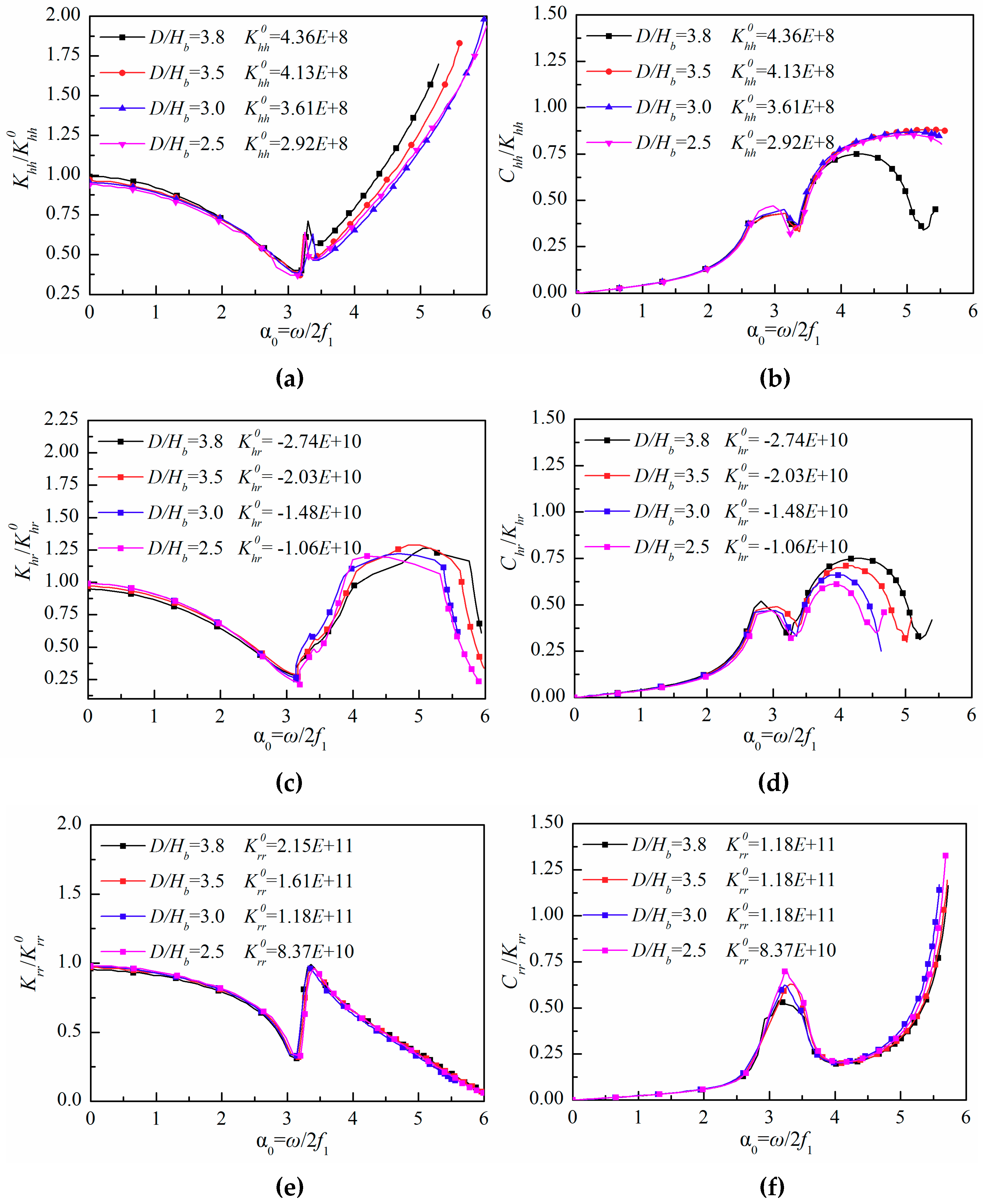
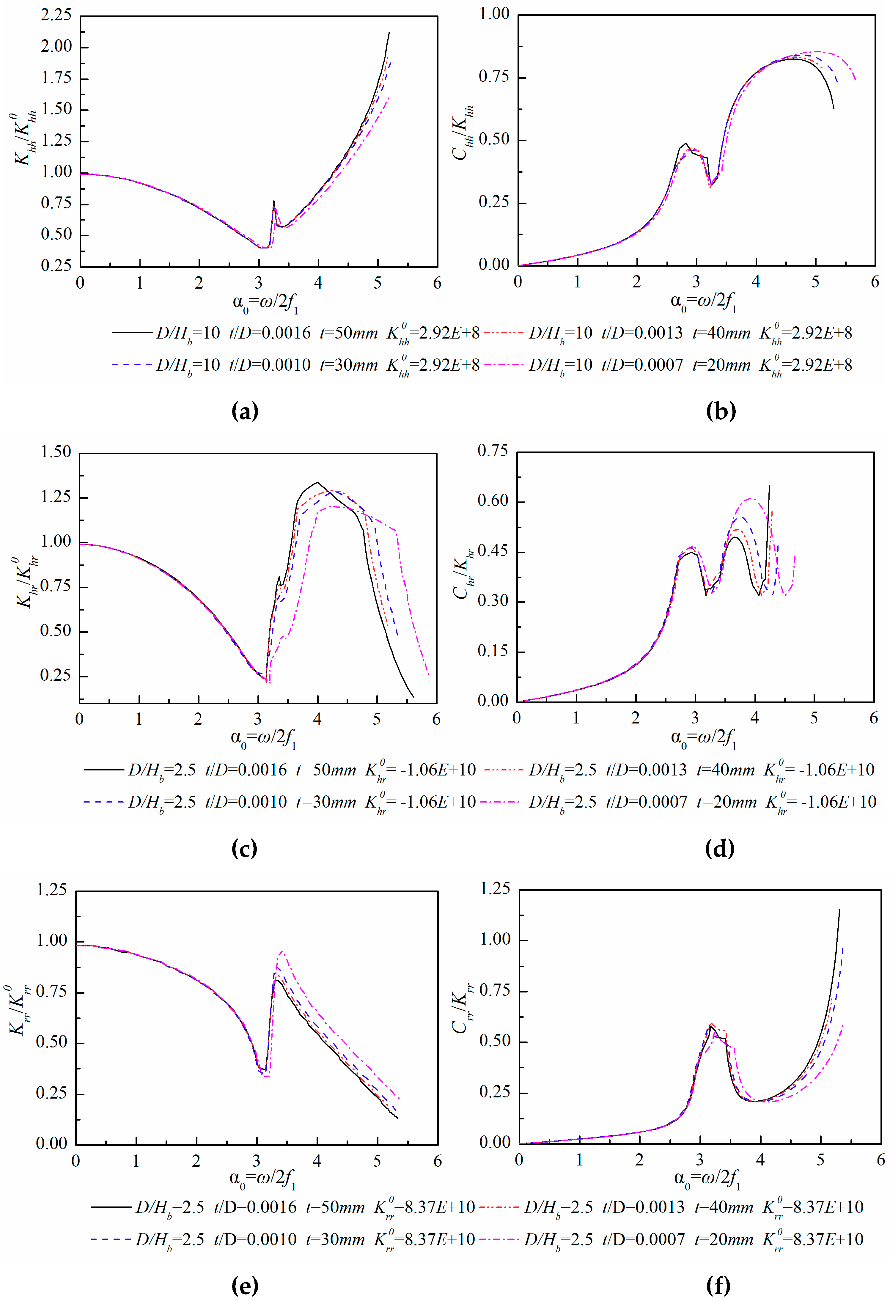
4.2. Influence of the Skirt Thickness

Figure 11 depicts the influence of the variation of the skirt thickness on the dynamic response of the WSBF (case 3,11–13, listed in Table 1). Before the first eigenfrequency, the overall dynamic impedance coefficients were hardly affected by the difference of skirt thickness. The trend of the horizontal dynamic stiffness coefficients described in Figure 11a appears that the increase of the stiffness coefficients becomes more distinct as the thickness increases when the frequency is larger than 4.5, but it is insensitive to the skirt thickness which is larger than 30 mm, where the solid black line indicates the skirt thickness for t = 50 mm, and the red dash line and blue dash line stand for the skirt thickness for t = 40 mm and t = 30 mm, respectively. The coupling stiffness coefficients depicted in Figure 11c are characterized by a higher slope as the thickness increases when the dimensionless frequency ranges from 3 to 5. Figure 11e plots the trends of the rocking stiffness, which shows that the first peak after the eigenfrequency becomes more marked as the thickness increases.
In regards to the dynamic damping coefficients, the thickness has significant influence on the horizontal and rocking at higher frequency range (larger than α0 > 4.5). It is an indication that the increase of the thickness results in the lower horizontal damping coefficient and the higher rocking damping.

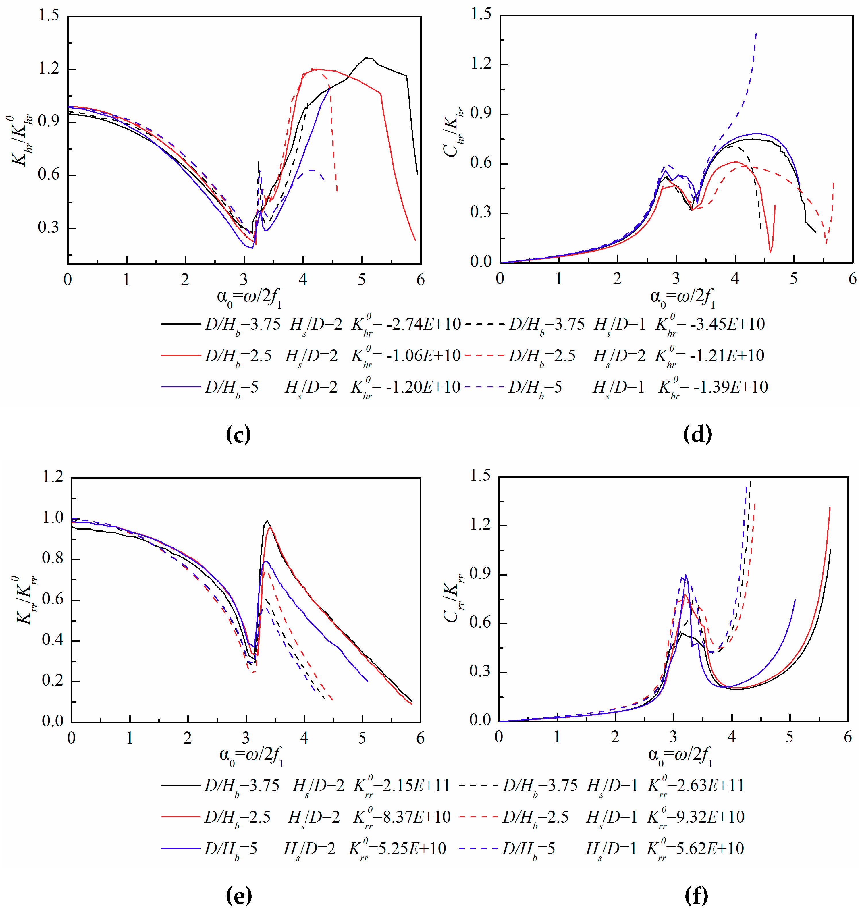
4.3. Influence of the Soil Thickness

To discuss the influence of soil layer thickness on the dynamic impedance of WSBF, it is investigated by keeping other dimensionless parameters constant and only changing the soil layer thickness, meanwhile three typical buckets with different relative slenderness ratios are selected. The variation of dynamic impedance coefficients with the frequency are described in Figure 12 (cases 2,3,7–10, listed in Table 1).
The dotted lines in Figure 12 indicate the dynamic impedances of foundation with soil thickness 30 m, and the solid lines represent the responses with 60 m soil layer. It can be seen from the comparison between the solid lines and the dotted lines, the soil thickness has a significant influence on the dynamic impedance. For the same slenderness ratio, the horizontal stiffness coefficients grow rapidly in the frequency range as the relative thickness decreases. The possible reason is that the greater the thickness of the soil layer is, the longer the vibration response transmits, and therefore the decay of the dynamic impedance is less noticeable. There are the same influences on the coupling and rocking coefficients. For rocking coefficients, the reduction slope becomes more marked as the relative thickness decreases after the first eigenfrequency. The coupling stiffness coefficients gradually display peaks against the thickness and decreases subsequently with the increase of excitation frequency.
Regarding the dynamic damping coefficients, the horizontal damping coefficient is less affected by the soil layer but mainly governed by the slenderness ratio. It can be seen from Figure 12f that the peaks of the rocking damping coefficients become more obvious as the relative soil thickness decreases. Meanwhile, the increasing pattern of the rocking damping coefficients after the first eigenfrequency is characterized by a higher slope against thickness. This behavior can be explained by the fact that more energy is dissipated because of the increase of the propagation distance. In conclusion, the results show that the relative soil layer thickness is the dominant factor affecting the dynamic impedances of the WSBF.

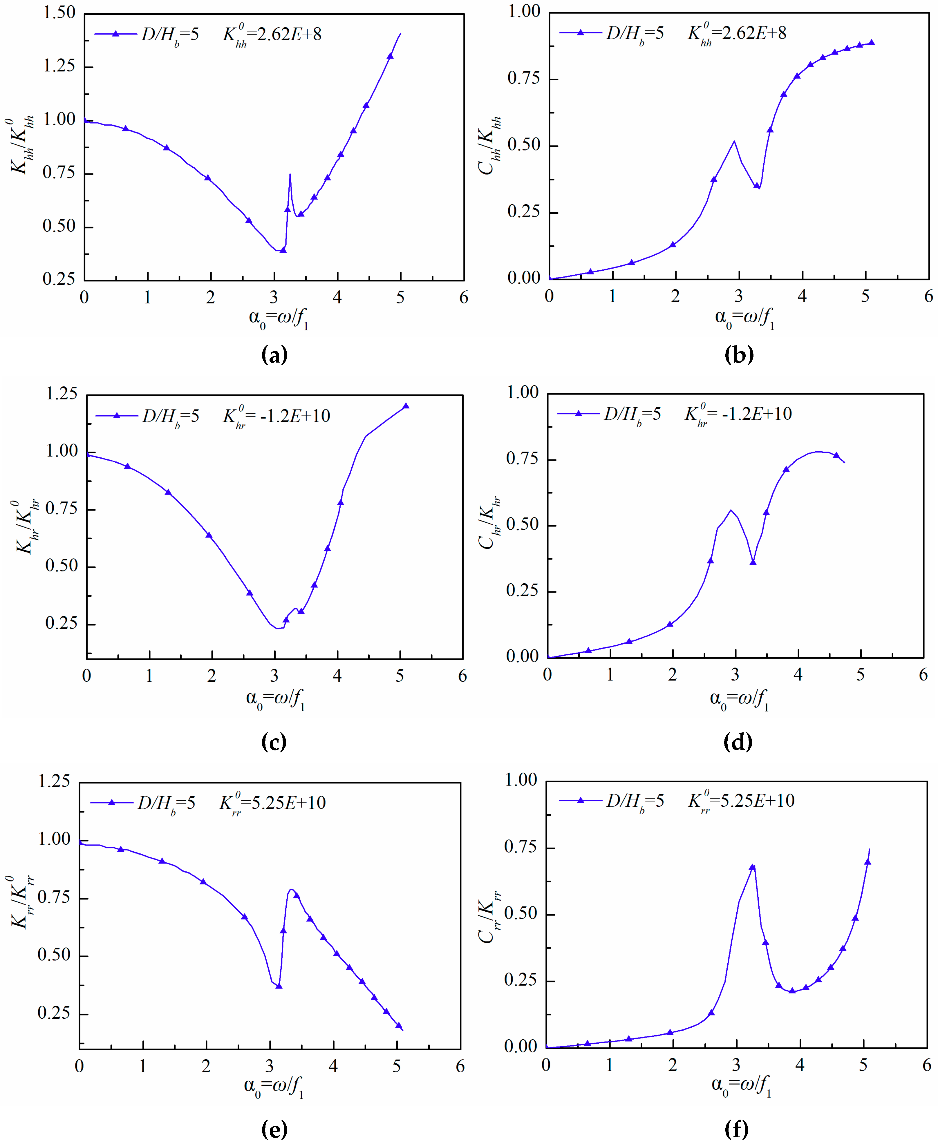
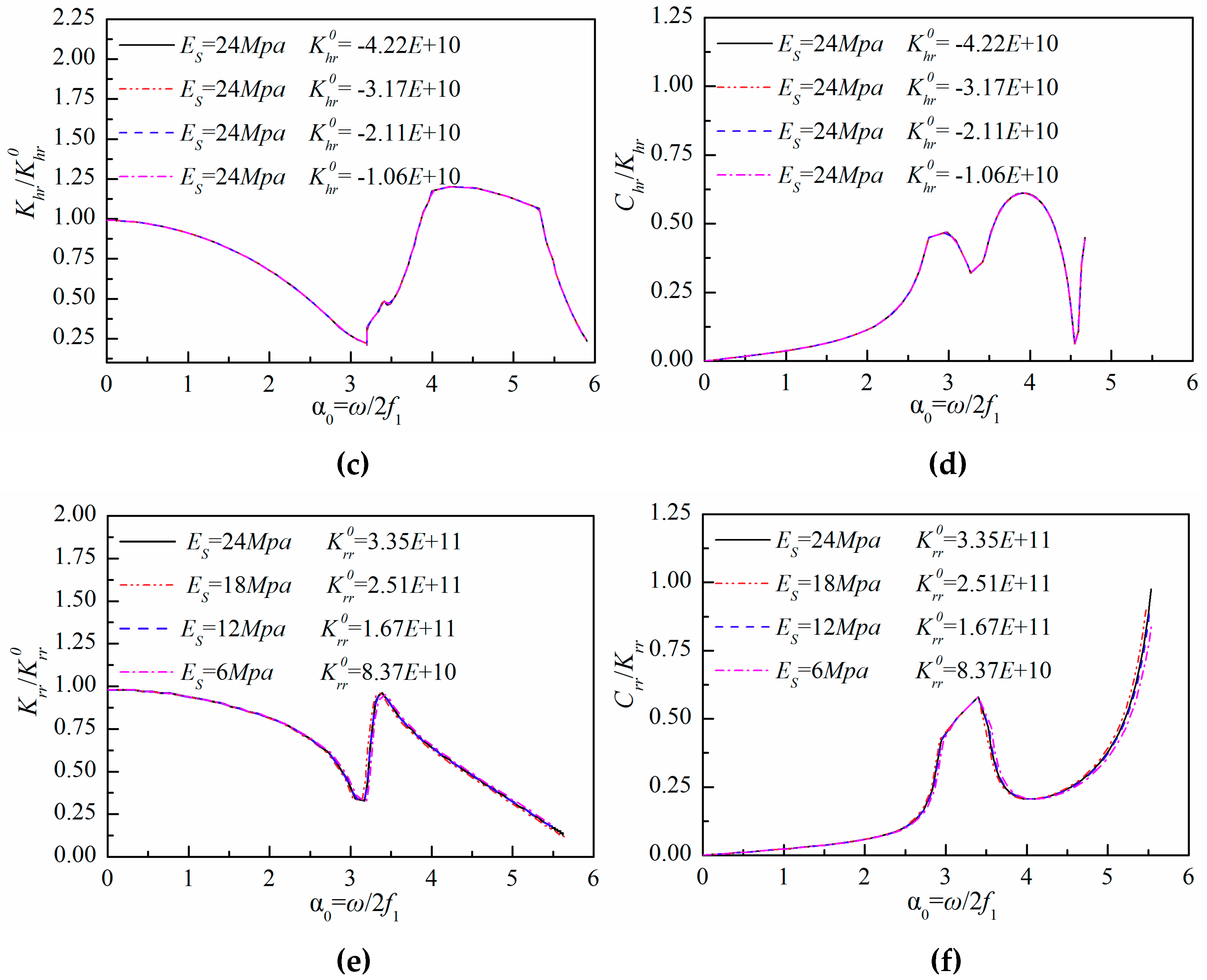
4.4. Influence of the Homogeneous Soil Stiffness

The trends of dynamic stiffness and damping coefficients with dimensionless excitation frequency under different stiffness of the homogeneous soil layer (profile A) with slenderness ratio D/Hb = 2.5 are depicted in Figure 13 (cases 4,14–16 listed in Table 1). The elastic modulus of the soil layer varies linearly from 6 MPa to 24 MPa. It is clear from Figure 13 that the dynamic impedances of the foundation have the same trends. This phenomenon shows that the dynamic impedance coefficients of WSBF are insensitive to the soil stiffness of homogeneous soil layers.

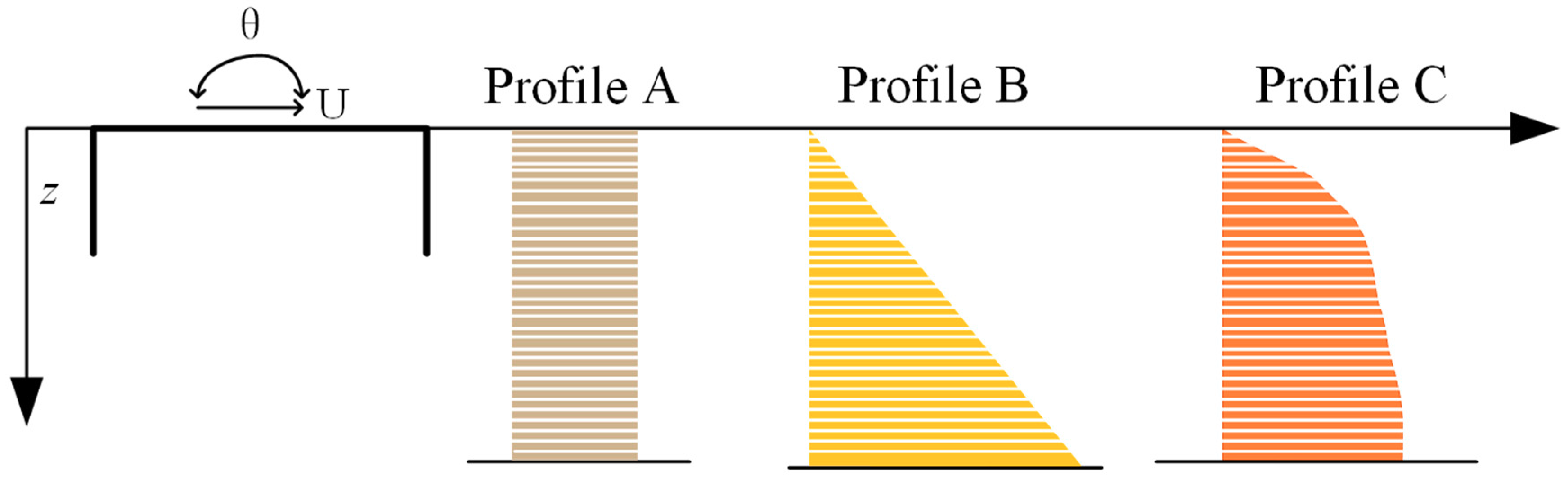
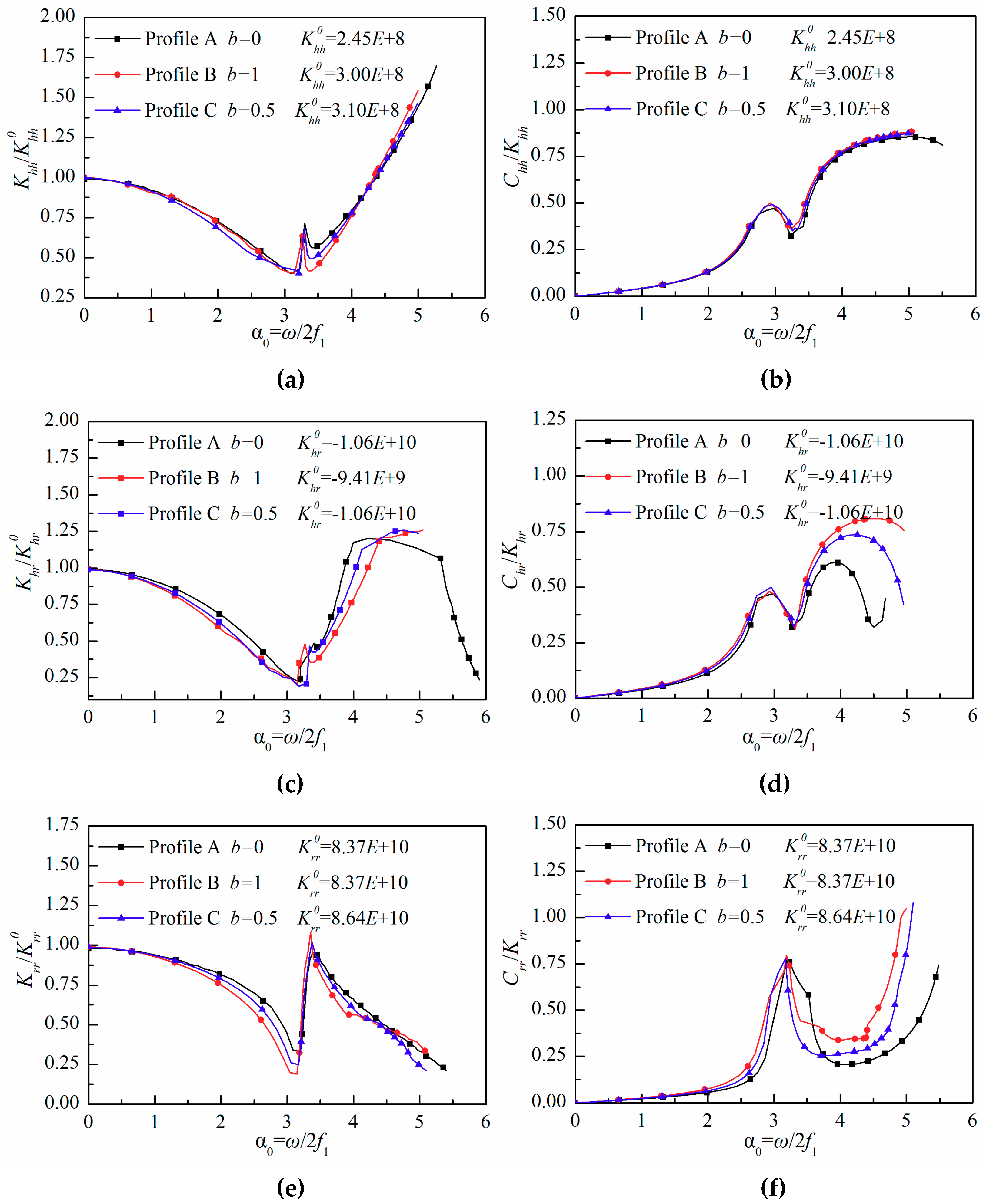
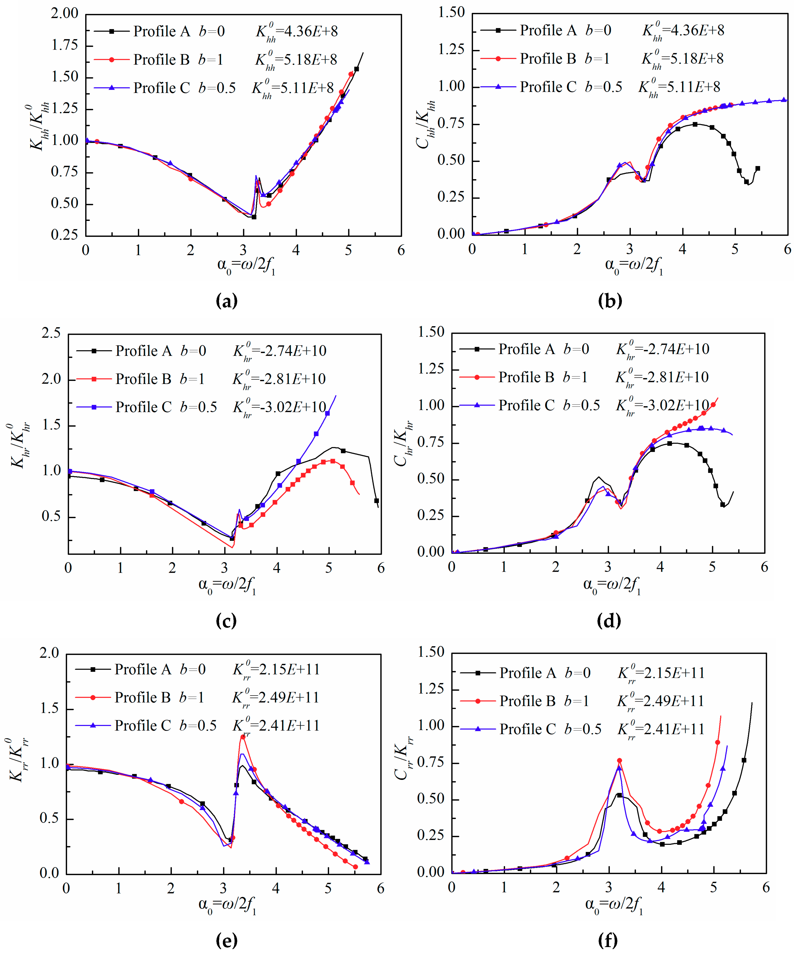
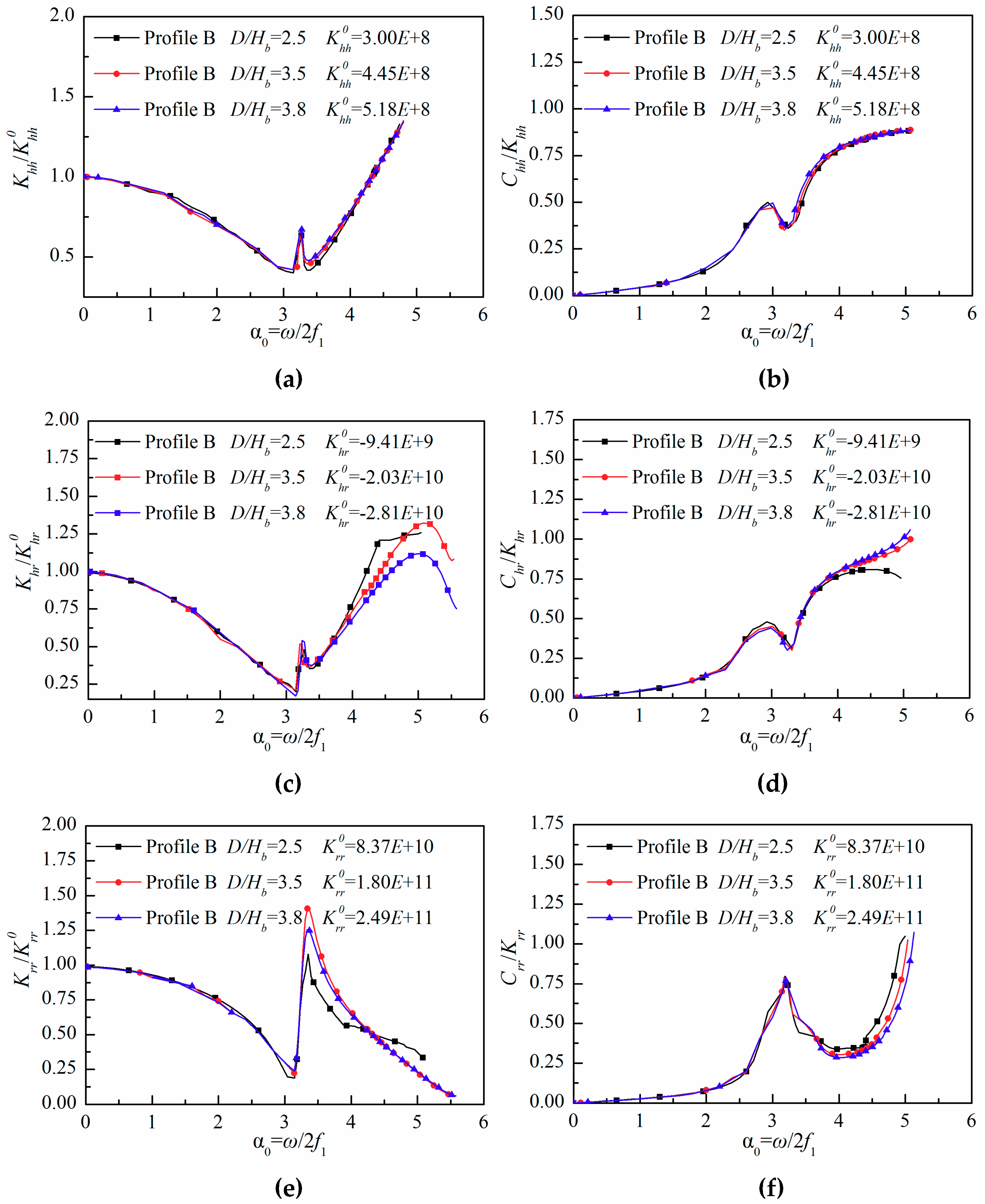
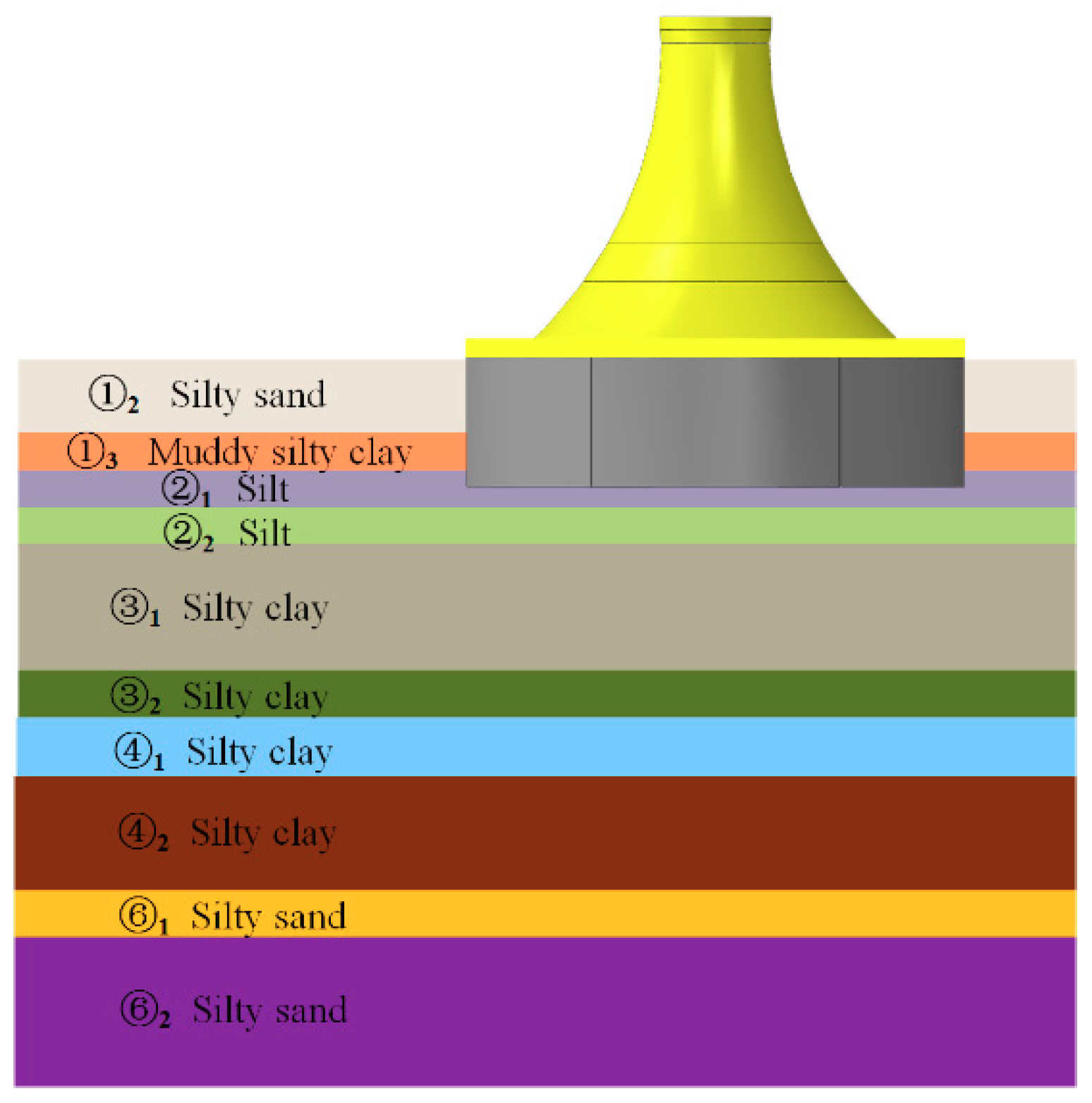
4.5. Influence of Multi-Layer Soil Stiffness

The effect of soil stiffness variation with depth in inhomogeneous soil layers on dynamic impedances of WSBF is depicted in Figure 14 (cases 3,17,20, listed in Table 1). The black lines plotted in Figure 14 indicate the dynamic impedances of WSBF embedded in profile A, red line and blue line represent the profile B and profile C, respectively. A common trend for all the dynamic stiffness coefficients was an observed drop before the first eigenfrequency. It can be seen that dropping in the rocking stiffness coefficient at the first eigenfrequency became more marked for profile B plotted in Figure 14e, while the coupling stiffness coefficient depicted in Figure 14c is characterized by a decreased slope for profile B. There is a suggestion that the increase of the soil stiffness in contact with the foundation would result in a higher stiffness coefficient.
For the imaginary part, the horizontal damping coefficient is not sensitive to the soil stiffness. The coupling and rocking damping coefficients are consistent with the real parts. For the higher frequency range (larger than α0 > 3.5), it shows that the increasing pattern of the damping coefficients is characterized by a higher slope for profile B after the first eigenfrequency. A possible explanation is that the dynamic impedances of foundation are mainly dependent on the soil stiffness where the foundation is embedded and the coupling and rocking coefficients are sensitive to the soil stiffness variation with depth.
Figure 15 plots the variations of three dynamic impedance coefficients under the effect of the multi-layer soil stiffness for WSBF with diameter 45 m (cases 10,19,22, listed in Table 1). The black, red, and blue lines depicted in Figure 15 represent, respectively, the dynamic impedances of WSBF embedded in profile A, profile B, and profile C. It can be seen that peaks of the rocking stiffness coefficients became more marked for profile B plotted in Figure 15e, while the coupling stiffness coefficients depicted in Figure 15c are characterized by a decreased slope for profile B after the first eigenfrequency. For the imaginary part, the coupling and rocking damping coefficients are sensitive to the multi-layer soil stiffness, while the horizontal damping coefficients are not. For the higher frequency range (larger than α0 > 3.5), it shows that the increasing pattern of the damping coefficients is characterized by a higher slope for profile B after the first eigenfrequency. The reason is that the dynamic impedances mainly depend on the multi-layer soil stiffness.
The effect of varying diameter is presented in Figure 16 (cases 17–19, listed in Table 1) and Figure 17 (cases 20–22, listed in Table 1), respectively, for profile B and profile C. The increasing of diameter affects marginally the horizontal dynamic impedance. The increasing of coupling stiffness coefficients depicted in Figure 16c is characterized by decreased slope as the diameter increases after the first eigenfrequency, and the coupling stiffness plotted in Figure 17c has the same trend. The rocking stiffness coefficients depicted in Figure 16e suggest that the decrease of the stiffness coefficients becomes more noticeable as the diameter increases, while the rocking stiffness plotted in Figure 17e is insensitive to the diameter. It indicates that the stiffness variation with depth is a more significant parameter than diameter in inhomogeneous soil.

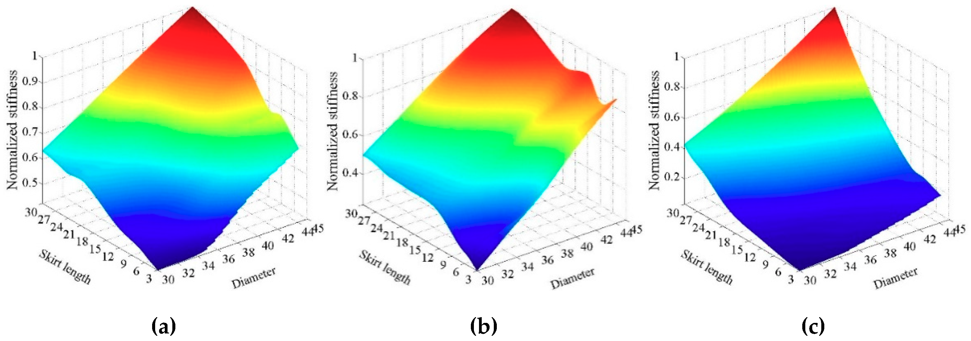
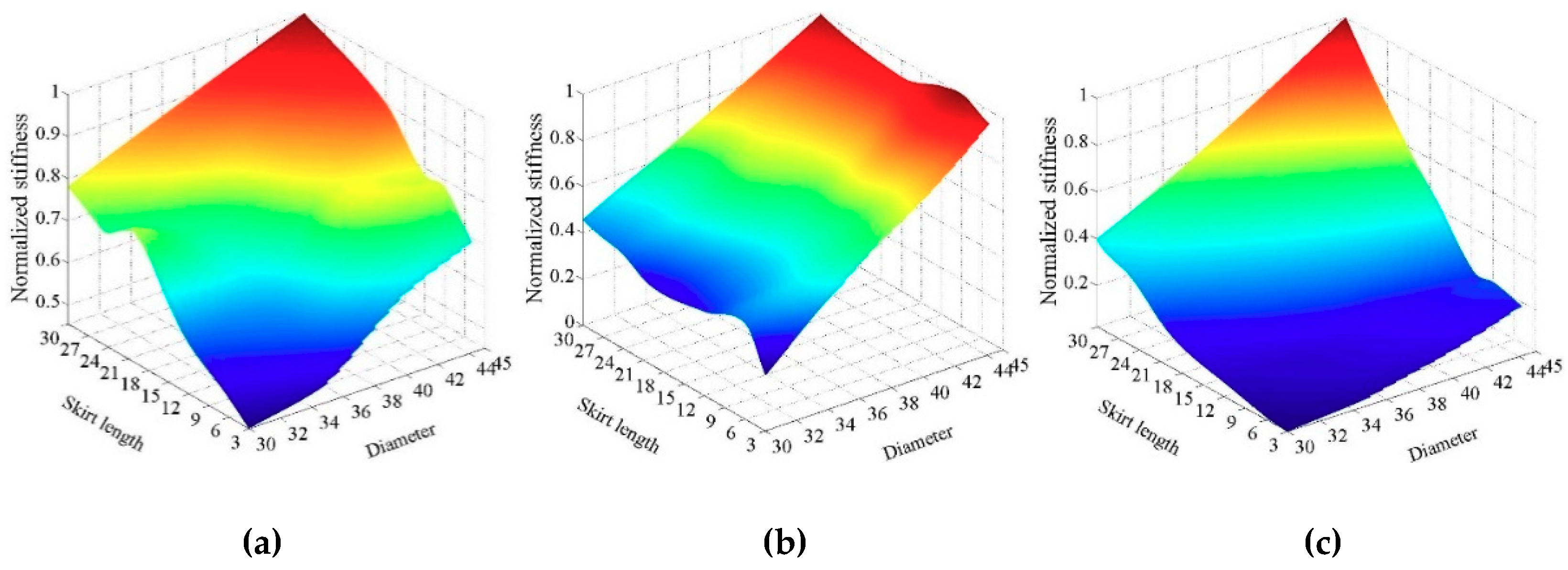
4.6. Multivariate Impact Analysis

Learning from above, the diameter and skirt length are the dominating factors for the design of OWT. The dynamic stiffness variation along with the different diameters and the skirt lengths under excitation load are discussed, to further illuminate the influence on the dynamic responses of WSBF. Firstly, the dimensionless excitation frequency of 0 was chosen as typical frequency because it states static stiffness variation along with the diameter and skirt length. Subsequently, the dynamic stiffness coefficients show an obvious decreasing trend before the first eigenfrequency (α0 < 3.0), so the dimensionless frequency of 2 away from resonance zone and static stiffness was also selected. Further, when the dimensionless frequency exceeds 3.5, the dimensionless frequency of 4 and 5 were both chosen to illustrate that the dynamic stiffness coefficients start to show different characteristics.
The variation of dynamic stiffness under a series of diameter and skirt length at the dimensionless excitation frequency 0 and 2 is displayed in Figure 18. The ordinate is normalized stiffness, which is foundation stiffness divided by the corresponding maximal stiffness. It can be seen from Figure 18a, the diameter is the main factor affecting the normalized horizontal stiffness, which increases with the diameter and skirt length. Figure 18b plots the coupling stiffness variation, the coupling stiffness decreases firstly and then increases against skirt increased, and the influence of the skirt length on the coupling stiffness is reduced as the diameter increases. Similarly, the rocking stiffness plotted in Figure 18c is also increased with the increase of the diameter and the skirt length, but the skirt length is the dominant factor.
The variation of dynamic stiffness with a series of diameter and skirt length excited by the dimensionless excitation frequency of 2 is depicted in Figure 19. It is shown that the variation trend of dynamic stiffness at dimensionless frequency of 2 is similar with the results at excitation frequency of 0. It is illustrated that the dynamic stiffness coefficients described in Figure 9 and Figure 10 have the same trend before the first eigenfrequency, so the dimensionless excitation frequency of 0 and 2 yield the similar normalized stiffness comparing Figure 18 with Figure 19.
The normalized horizontal stiffness variation under dimensionless frequency 4 is shown in Figure 20a, which increases with the diameter increasement when the diameter is larger than 36 m. According to Figure 20b, it can be seen that the skirt length has less influence on the coupling stiffness which is mainly governed by the diameter when the skirt length reaches 9 m. The normalized rocking stiffness is mainly controlled by the skirt length.
Different from the previous three typical frequencies, the horizontal stiffness showned in Figure 21a is affected profoundly by the skirt length, and the diameter infuences the stiffness only when it is larger than 36 m. It can be clearly observed from Figure 21b that coupling stiffness is mainly governed by the diameter. The rocking stiffness depicted in Figure 21c is still controlled by the skirt length, especially for the larger diameter.

5. Engineering Verification
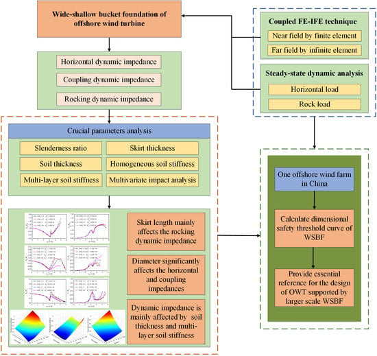
To illustrate the influence of soil-structure interaction on the foundation design, one offshore wind farm, which is approximately 45 km off the coast of the Yellow Sea in China, with the water depth of 8–15 m, was selected to be the research object. The installed capacity of the offshore wind farm is 300 MW, and 11 wind turbines with rated power of 3.3 MW supported by the WSBF were constructed. The serial numbers of wind turbines are 40#–43#, 45#–47# and 51#–54#.
The maximum allowable tilt of monopile at seabed level is ±0.5° as suggested in DNV-OS-J101 [3]. However, the control standard of WSBF should be considered as more stringent than monopole foundation with the maximum allowable tilt value as 0.25° because the typical construction tolerances always range from 0.2° to 0.25° [48]. Further, the geometrical safety threshold of the WSBF, which is located above the offshore wind farm, was calculated based on the maximum allowable tilt and control load in order to meet the design criteria. The control load can be obtained by the wind turbine manufacturer and the soil profile of the actual drill hole is presented in Figure 22. The main parameters of soil are shown in Table 2.
The calculated safety threshold curve of WSBF depicted in Figure 23 is built by coupling FE-IFE technique with the allowable tilt at the foundation head of 0.25°. The blue solid line and the red triangle symbols represent the safety threshold of the foundation geometric size and the dimensions of WSBF applied in offshore wind farm, respectively. The pink dotted lines are described to obtain the allowable minimum design value of the diameter and skirt length which are determined as 29 m and 7.5 m respectively. It is also clearly found that the increasing pattern of skirt length becomes less marked when the diameter exceeds 33 m, and the foundation stability has been mainly controlled by the diameter. The red triangle symbols indicate that the design geometries of WSBF all located above the blue threshold curve with the diameters ranging from 32 m to 36 m and the skirt lengths ranging from 9 m to 13 m. It is explained that the calculated dimensional safety threshold curve can be considered to be reasonable and correct and provide offshore wind turbine design with a reference to improve the design efficiency.

6. Conclusions

Given the importance of the frequency-dependent dynamic impedances, including horizontal, rocking, and coupling impedance, in accurate evaluation of the dynamic response of the WSBF, this study deploys the FE-IFE technique to conduct a parametric investigation, analyzing the influence of the slenderness ratio, the skirt thickness, the relative soil thickness, and the soil stiffness. The main conclusions can be summarized as follows:
(1)
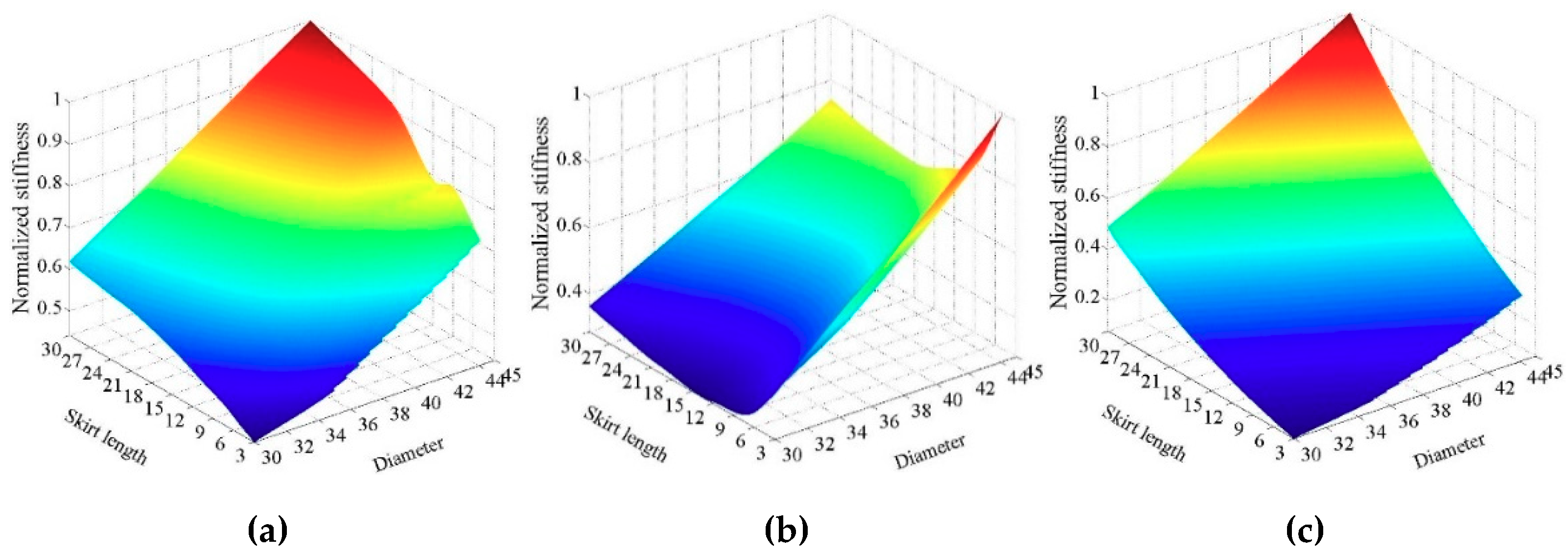
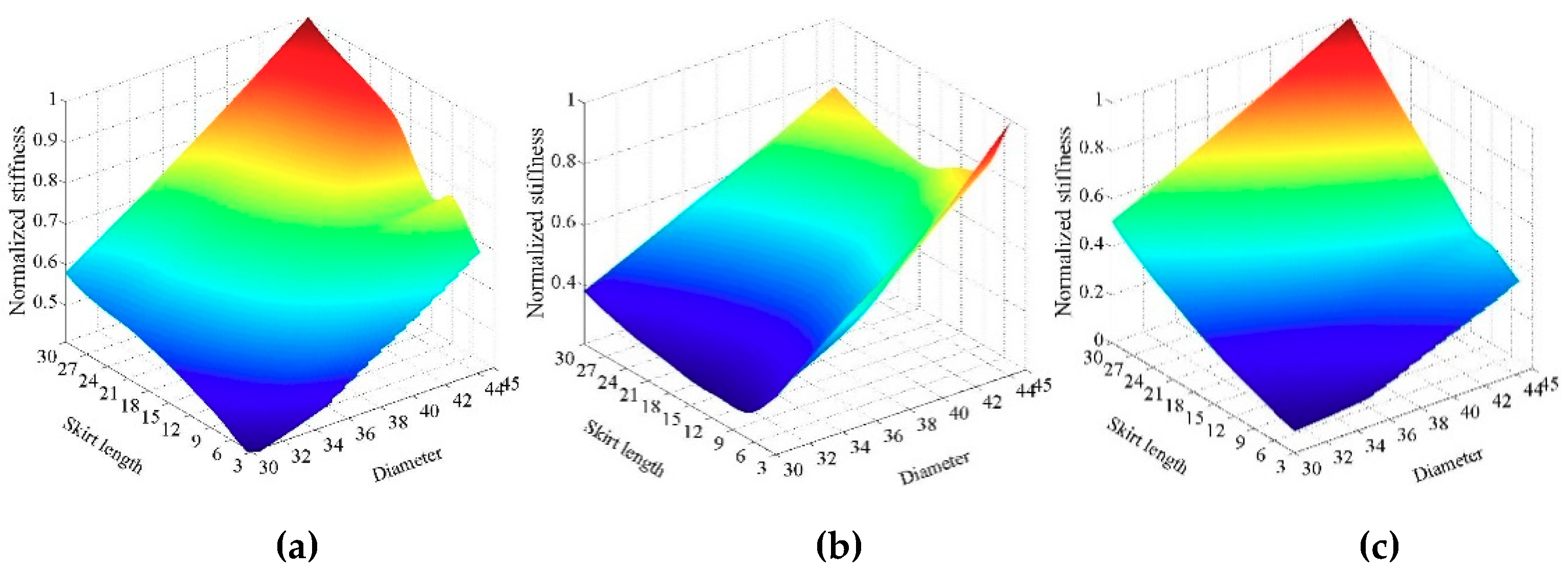
Firstly, the slenderness ratio significantly affects the dynamic impedances of WSBF. After the first eigenfrequency, the coupling stiffness increases sharply and the rocking stiffness decreases smoothly by increasing skirt length, as more rotation and less lateral contribute to the dynamic response. On the contrary, the horizontal stiffness coefficient grows remarkedly against diameter, because the horizontal vibration is mainly transmitted to the surrounding soil at relatively shallow area, enhancing the horizontal stiffness of the WSBF. As for the skirt thickness, when it is larger than 30 mm, its impact on the dynamic impedance of WSBF can be negligible.
(2)
Secondly, within the frequency range investigated, the dynamic impedances of the foundation are marginally affected by the relative stiffness of homogeneous soil, but more sensitive to the relative soil thickness. This can be explained by the fact that the larger the soil thickness is, the longer the vibration response transmits, and therefore the decay of the dynamic impedance is less noticeable. For the multi-layer soil profile, the coupling and rocking coefficients are more sensitive to the soil stiffness variation with depth because the dynamic impedances depend on the soil stiffness where the foundation is embedded.
(3)
Additionally, both the diameter and skirt length are found to be substantial parameters to the horizontal stiffness and coupling stiffness, while the rocking stiffness is mainly determined by the skirt length in the frequency range considered. The horizontal stiffness under the dimensionless frequency of 4 and 5 is governed by the diameter when it is greater than 36 m. The coupling stiffness under the dimensionless frequency of 0 and 2 decreases firstly and then increases with the skirt length increasing.
(4)
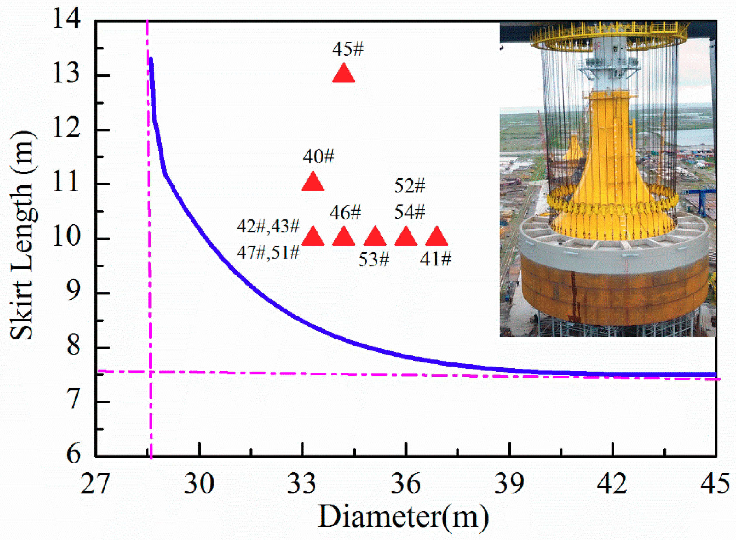
Lastly, taking one OWF in China as an example, the dimensional safety threshold curve is calculated based on the maximum allowable tilt of WSBF and corresponding design load. According to proposed curve, the minimum values of the diameter and skirt length are determined as 29 m and 7.5 m, respectively. The calculated dimensional safety threshold curve proves to be reasonable and correct because the actual design geometries of WSBF all locate above the threshold values.

Author Contributions

Conceptualization, J.L.; methodology, X.D., Q.J. and Y.Z.; formal analysis, Q.J., X.D. and H.Z.; software, Q.J. and H.Z; resources, X.D. and Q.J.; data curation, X.D.; writing—original draft preparation, Q.J.; writing—review and editing, X.D., H.Z. and Y.Z.; supervision, J.L.; validation, X.D.; funding acquisition, J.L. and X.D.

Funding

This research was supported by the Fund for National Natural Science Foundation of China (51709202) and Innovation Method Fund of China (Grant No. 2016IM030100).

Acknowledgments

All workers from the State Key Laboratory of Hydraulic Engineering Simulation and Safety of Tianjin University are acknowledged. The writers acknowledge the assistance of anonymous reviewers as well.

Conflicts of Interest

The authors declare no conflict of interest.

References

  1. Wang, X.Y.; Zeng, X.W.; Li, J.L.; Yang, X.; Wang, H.J. A review on recent advancements of substructures for offshore wind turbines. Energy Convers. Manag. 2018, 158, 103–119. [Google Scholar] [CrossRef]
  2. Lian, J.J.; Cai, O.; Dong, X.F.; Jiang, Q.; Zhao, Y. Health Monitoring and Safety Evaluation of the Offshore Wind Turbine Structure: A Review and Discussion of Future Development. Sustainability 2019, 11, 494. [Google Scholar] [CrossRef]
  3. Swagata, B.; Sumanta, H. Design of monopile supported offshore wind turbine in clay considering dynamic soil–structure-interaction. Soil Dyn. Earthq. Eng. 2015, 73, 103–117. [Google Scholar]
  4. Arany, L.; Bhattacharya, S.; Macdonald, J.; Hogan, S.J. Design of monopiles for offshore wind turbines in 10 steps. Soil Dyn. Earthq. Eng. 2017, 92, 126–152. [Google Scholar] [CrossRef]
  5. Bisoi, S.; Haldar, S. Dynamic analysis of offshore wind turbine in clay considering soil–monopile–tower interaction. Soil Dyn. Earthq. Eng. 2014, 63, 19–35. [Google Scholar] [CrossRef]
  6. Carswell, W.; Arwade, S.R.; DeGroot, D.J.; Lackner, M.A. Soil-structure reliability of offshore wind turbine monopile foundations. Wind Energy 2015, 18, 483–498. [Google Scholar] [CrossRef]
  7. Santangelo, F.; Failla, G.; Santini, A.; Arena, F. Time-domain uncoupled analyses for seismic assessment of land-based wind turbines. Eng. Struct. 2016, 123, 275–299. [Google Scholar] [CrossRef]
  8. Haciefendioglu, K. Stochastic seismic response analysis of offshore wind turbine including fluid-structure-soil-interaction. Struct. Des. Tall Spec. Build. 2012, 21, 867–878. [Google Scholar] [CrossRef]
  9. Alati, N.; Failla, G.; Arena, F. Seismic analysis of offshore wind turbines on bottom-fixed support structures. Philos. Trans. R. Soc. A 2015, 373, 20140086. [Google Scholar] [CrossRef]
  10. Jalbi, S.; Nikitas, G.; Bhattacharya, S.; Alexander, N. Dynamic design considerations for offshore wind turbine jackets supported on multiple foundations. Mar. Struct. 2019, 67, 102631. [Google Scholar] [CrossRef]
  11. Yang, J.; He, E.M.; Hu, Y.Q. Dynamic modeling and vibration suppression for an offshore wind turbine with a tuned mass damper in floating platform. Appl. Ocean Res. 2019, 83, 21–29. [Google Scholar] [CrossRef]
  12. Lian, J.J.; Chen, F.; Wang, H.J. Laboratory tests on soil-skirt interaction and penetration resistance of suction caissons during installation in sand. Ocean Eng. 2014, 84, 1–13. [Google Scholar] [CrossRef]
  13. Zhang, P.Y.; Ding, H.Y.; Le, C.H. Seismic response of large-scale prestressed concrete bucket foundation for offshore wind turbines. J. Renew. Sustain. Energy 2014, 6, 013127. [Google Scholar] [CrossRef]
  14. Dong, X.; Lian, J.; Wang, H.; Yu, T.; Zhao, Y. Structural vibration monitoring and operational modal analysis of offshore wind turbine structure. Ocean Eng. 2018, 150, 280–297. [Google Scholar] [CrossRef]
  15. Liu, M.; Lian, J.J.; Yang, M. Experimental and numerical studies on lateral bearing capacity of bucket foundation in saturated sand. Ocean Eng. 2017, 144, 14–20. [Google Scholar] [CrossRef]
  16. Wang, X.; Zhang, P.; Ding, H.; Liu, R. Experimental study of the accumulative deformation effect on wide-shallow composite bucket foundation for offshore wind turbines. J. Renew. Sustain. Energy 2017, 9, 063306. [Google Scholar] [CrossRef]
  17. Ibsen, L.B. Implementation of a new foundations concept for offshore wind farms. In Proceedings of the 15th Nordic Geotechnical Meeting, Sandefjord, Norway, 3–6 Septemner 2008; pp. 19–33. [Google Scholar]
  18. Dong, X.; Lian, J.; Yang, M.; Wang, H. Operational modal identification of offshore wind turbine structure based on modified stochastic subspace identification method considering harmonic interference. J. Renew. Sustain. Energy 2014, 6, 033128. [Google Scholar] [CrossRef]
  19. Lian, J.J.; Jiang, J.N.; Dong, X.F.; Wang, H.J.; Zhou, H.; Wang, P.W. Coupled Motion Characteristics of Offshore Wind Turbines during the Integrated Transportation Process. Energies 2019, 12, 2023. [Google Scholar] [CrossRef]
  20. Wolf, J.P.; Song, C. Some cornerstones of dynamic soil–structure interaction. Eng. Struct. 2002, 24, 13–28. [Google Scholar] [CrossRef]
  21. Novak, M.; Nogamit, T. Soil-pile interaction in horizontal vibration. Earthq. Eng. Struct. Dyn. 1977, 5, 263–281. [Google Scholar] [CrossRef]
  22. Torabi, H.; Rayhani, M.T. Equivalent-linear pile head impedance functions using a hybrid method. Earthq. Eng. Struct. Dyn. 2017, 101, 137–152. [Google Scholar] [CrossRef]
  23. Harte, M.; Basu, B.; Nielsen, S.R.K. Dynamic analysis of wind turbines including soil-structure interaction. Eng. Struct. 2012, 45, 509–518. [Google Scholar] [CrossRef]
  24. Latini, C.; Zania, V.; Johannesson, B. Dynamic stiffness and damping of foundation for jacket structures. In Proceedings of the 6th International Conference on Earthquake Geotechnical Engineering, Christchurch, New Zealand, 1–4 November 2015. [Google Scholar]
  25. Latini, C.; Zania, V.; Cisternino, M. Dynamic stiffness of horizontally vibrating suction caissons. In Proceedings of the 17th Nordic Geotechnical Meeting, Reykjavik, Icelan, 25–28 May 2016; pp. 973–982. [Google Scholar]
  26. Latini, C.; Zania, V. Dynamic lateral response of suction caissons. Soil Dyn. Earthq. Eng. 2017, 100, 59–71. [Google Scholar] [CrossRef]
  27. Gerolymos, N.; Gazetas, G. Static and dynamic response of massive caisson foundations with soil and interface nonlinearities-validation and results. Soil Dyn. Earthq. Eng. 2006, 26, 377–394. [Google Scholar] [CrossRef]
  28. Gerolymos, N.; Gazetas, G. Winkler model for lateral response of rigid caisson foundations in linear soil. Soil Dyn. Earthq. Eng. 2006, 26, 347–361. [Google Scholar] [CrossRef]
  29. Gerolymos, N.; Gazetas, G. Development of Winkler model for static and dynamic response of caisson foundations with soil and interface nonlinearities. Soil Dyn. Earthq. Eng. 2006, 26, 363–376. [Google Scholar] [CrossRef]
  30. Damgaard, M.; Andersen, L.V.; Ibsen, L.B. Assessment of dynamic substructuring of a wind turbine foundation applicable for aeroelastic simulations. Wind Energy 2015, 18, 1387–1401. [Google Scholar] [CrossRef]
  31. Damgaard, M.; Andersen, L.V.; Ibsen, L.B. Dynamic response sensitivity of an offshore wind turbine for varying subsoil conditions. Ocean Eng. 2015, 101, 227–234. [Google Scholar] [CrossRef]
  32. Andersen, L.; Ibse, L.B.; Liingaard, M.A. Impedance of Bucket Foundations-Torsional, Horizontal and Rocking Motion. In Proceedings of the Sixth International Conference on Engineering Computational Technology, Stirlingshire, UK, 2–5 September 2008; pp. 2–5. [Google Scholar]
  33. Wang, H.; Liu, W.; Zhou, D.; Wang, S.; Du, D. Lumped-parameter model of foundations based on complex Chebyshev polynomial fraction. Soil Dyn. Earthq. Eng. 2013, 50, 192–203. [Google Scholar] [CrossRef]
  34. Liingaard, M.; Andersen, L.; Ibsen, L.B. Impedance of flexible suction caissons. Earthq. Eng. Struct. Dyn. 2007, 36, 2249–2271. [Google Scholar] [CrossRef]
  35. Liingaard, M. Dynamic Behaviour of Suction Caissons. Ph.D. Thesis, Aalborg University, Aalborg, Denmark, 19 October 2006. [Google Scholar]
  36. He, R.; Zhang, J.; Chen, W. Using the Elastic Vertical Vibration of a Rigid Caisson at Low Frequencies to Stabilize the Foundation of Coastal Engineering Structures. J. Coastal Res. 2017, 33, 989–996. [Google Scholar] [CrossRef]
  37. He, R.; Pak, R.Y.S.; Wang, L.Z. Elastic lateral dynamic impedance functions for a rigid cylindrical shell type foundation. Int. J. Numer. Anal. Method. Geomech. 2017, 41, 508–526. [Google Scholar] [CrossRef]
  38. Doherty, J.P.; Houlsby, G.T.; Deeks, A.J. Stiffness of Flexible Caisson Foundations Embedded in Nonhomogeneous Elastic Soil. J. Geotech. Geoenviron. Eng. 2005, 131, 1498–1508. [Google Scholar] [CrossRef]
  39. Ba, Z.; Liang, J.; Lee, V.W.; Kang, Z. Dynamic impedance functions for a rigid strip footing resting on a multi-layered transversely isotropic saturated half-space. Eng. Anal. Bound. Elem. 2018, 86, 31–44. [Google Scholar] [CrossRef]
  40. Liu, M.; Yang, M.; Wang, H. Bearing behavior of wide-shallow bucket foundation for offshore wind turbines in drained silty sand. Ocean Eng. 2014, 82, 169–179. [Google Scholar] [CrossRef]
  41. Veritas. DNV-OS-J101-Design of Offshore Wind Turbine Structures; Det Norske Veritas: Oslo, Norway, 2004. [Google Scholar]
  42. IEC 61400-3. Wind Turbines-Part 3: Design Requirements for Offshore Wind Turbines; International Electrotechnical Commission: Geneva, Switzerland, 2009. [Google Scholar]
  43. Yang, Y.B.; Hung, H.H. A 2.5D finite/infinite element approach for modelling visco-elastic bodies subjected to moving loads. Int. J. Numer. Method. Eng. 2001, 51, 1317–1336. [Google Scholar] [CrossRef]
  44. Wang, G.; Chen, L.; Song, C. Finite–infinite element for dynamic analysis of axisymmetrically saturated composite foundations. Int. J. Numer. Method. Eng. 2006, 67, 916–932. [Google Scholar] [CrossRef]
  45. Versteijlen, W.G.; Van Dalen, K.N.; Metrikine, A.V.; Hamre, L. Assessing the small-strain soil stiffness for offshore wind turbines based on in situ seismic measurements. J. Phys. Conf. Ser. 2014, 524, 012088. [Google Scholar] [CrossRef] [Green Version]
  46. Kuhlemeyer, R.L.; Lysmer, J. Finite element method accuracy for wave propagation problems. J. Soil Mech. Found. Div. 1973, 99, 421–427. [Google Scholar]
  47. Doherty, J.P.; Deeks, A.J. Elastic response of circular footings embedded in a non-homogeneous half-space. Geotechnique 2003, 8, 703–714. [Google Scholar] [CrossRef]
  48. Jung, S.; Kim, S.R.; Patil, A.; Hung, L.C. Effect of monopile foundation modeling on the structural response of a 5-MW offshore wind turbine tower. Ocean Eng. 2015, 109, 479–488. [Google Scholar] [CrossRef] [Green Version]
Figure 1. The prototypes of wide-shallow bucket foundation: (a) Frederikshavn, Denmark [17]; (b) Xiangshui, China.
Energies 12 04370 g001
Figure 2. Illustration of four different foundation types: (a) End pile; (b) floating piles; (c) suction caisson; (d) wide-shallow bucket foundations (WSBF). Note: Hs denotes thickness of soil layer, Hp denotes skirt length of pile and suction caisson, Hb denotes skirt length of WSBF.
Energies 12 04370 g002
Figure 3. Schematic of the WSBF under horizontal force and moment action: (a) Force and moment (b) displacement and rotation.
Energies 12 04370 g003
Figure 4. Two-dimensional coupling numerical model of WSBF in the finite and infinite element domains.
Energies 12 04370 g004
Figure 5. Coupling model combined finite element with an infinite element domain.
Energies 12 04370 g005
Figure 6. The finite-infinite element (FE-IFE) model of WSBF.
Energies 12 04370 g006
Figure 7. Variation of three dynamic impedance coefficients with respect to the dimensionless frequency: (a) Horizontal stiffness coefficient; (b) horizontal damping coefficient; (c) coupling stiffness coefficient; (d) coupling damping coefficient; (e) rocking stiffness coefficient; (f) rocking damping coefficient.
Energies 12 04370 g007
Figure 8. Soil profiles considered for dynamic impedances of WSBF.
Energies 12 04370 g008
Figure 9. Variation of three dynamic impedance coefficients with respect to the dimensionless frequency under effect of the slenderness ratio by varying the skirt length: (a) Horizontal stiffness coefficient; (b) horizontal damping coefficient; (c) coupling stiffness coefficient; (d) coupling damping coefficient; (e) rocking stiffness coefficient; (f) rocking damping coefficient.
Energies 12 04370 g009
Figure 10. Variation of three dynamic impedance coefficients with respect to the dimensionless frequency under different diameter of WSBF: (a) Horizontal stiffness coefficient; (b) horizontal damping coefficient; (c) coupling stiffness coefficient; (d) coupling damping coefficient; (e) rocking stiffness coefficient; (f) rocking damping coefficient.
Energies 12 04370 g010
Figure 11. Variation of three dynamic impedance coefficients with respect to the dimensionless frequency under different skirt thickness: (a) Horizontal stiffness coefficient; (b) horizontal damping coefficient; (c) coupling stiffness coefficient; (d) coupling damping coefficient; (e) rocking stiffness coefficient; (f) rocking damping coefficient.
Energies 12 04370 g011
Figure 12. Variation of three dynamic impedance coefficients with respect to the dimensionless frequency under the effect of the relative thickness of the soil layer: (a) Horizontal stiffness coefficient; (b) horizontal damping coefficient; (c) coupling stiffness coefficient; (d) coupling damping coefficient; (e) rocking stiffness coefficient; (f) rocking damping coefficient.
Energies 12 04370 g012aEnergies 12 04370 g012b
Figure 13. Variation of three dynamic impedance coefficients with respect to the dimensionless frequency under the effect of the relative homogeneous soil stiffness: (a) Horizontal stiffness coefficient; (b) horizontal damping coefficient; (c) coupling stiffness coefficient; (d) coupling damping coefficient; (e) rocking stiffness coefficient; (f) rocking damping coefficient.
Energies 12 04370 g013aEnergies 12 04370 g013b
Figure 14. Variation of three dynamic stiffness coefficients with respect to the dimensionless frequency under the effect of the multi-layer soil stiffness: (a) Horizontal stiffness coefficient; (b) horizontal damping coefficient; (c) coupling stiffness coefficient; (d) coupling damping coefficient; (e) rocking stiffness coefficient; (f) rocking damping coefficient.
Energies 12 04370 g014
Figure 15. Variation of three dynamic stiffness coefficients with respect to the dimensionless frequency under the effect of the multi-layer soil stiffness for WSBF with diameter 45 m: (a) Horizontal stiffness coefficient; (b) horizontal damping coefficient; (c) coupling stiffness coefficient; (d) coupling damping coefficient; (e) rocking stiffness coefficient; (f) rocking damping coefficient.
Energies 12 04370 g015
Figure 16. Variation of three dynamic impedance coefficients with respect to the dimensionless frequency under different diameter of WSBF embedded in Profile B: (a) Horizontal stiffness coefficient; (b) horizontal damping coefficient; (c) coupling stiffness coefficient; (d) coupling damping coefficient; (e) rocking stiffness coefficient; (f) rocking damping coefficient.
Energies 12 04370 g016
Figure 17. Variation of three dynamic impedance coefficients with respect to the dimensionless frequency under different diameter of WSBF embedded in Profile C: (a) Horizontal stiffness coefficient; (b) horizontal damping coefficient; (c) coupling stiffness coefficient; (d) coupling damping coefficient; (e) rocking stiffness coefficient; (f) rocking damping coefficient.
Energies 12 04370 g017aEnergies 12 04370 g017b
Figure 18. Variation of three dynamic stiffness coefficients at dimensionless excitation frequency of 0 and 2: (a) Horizontal stiffness; (b) coupling stiffness; (c) rocking stiffness.
Energies 12 04370 g018
Figure 19. Variation of three dynamic stiffness coefficients at dimensionless excitation frequency of 2: (a) Horizontal stiffness; (b) coupling stiffness; (c) rocking stiffness.
Energies 12 04370 g019
Figure 20. Variation of three dynamic stiffness coefficients at dimensionless excitation frequency of 4: (a) Horizontal stiffness; (b) coupling stiffness; (c) rocking stiffness.
Energies 12 04370 g020
Figure 21. Variation of three dynamic stiffness coefficients at dimensionless excitation frequency of 5: (a) Horizontal stiffness; (b) coupling stiffness; (c) rocking stiffness.
Energies 12 04370 g021
Figure 22. Soil profile parameters and WSBF.
Energies 12 04370 g022
Figure 23. The dimensional safety threshold curve of WSBF.
Energies 12 04370 g023
Table 1. Parameters and cases selected in the parametric analysis.
CasesD (m)Hb (m)D/HbHs (m)Hs/Dt (mm)t/DSoil ProfileEs (MPa)
13031060220/A6
2306560220/A6
330122.5602200.0007A6
430201.560220/A6
535123.0601.720/A6
640123.3601.520/A6
745123.75601.320/A6
8306530120/A6
930122.530120/A6
1045123.75300.720/A6
1130122.5602300.0010A6
1230122.5602400.0013A6
1330122.5602500.0016A6
1430122.560220/A12
1530122.560220/A18
1630122.560220/A24
1730122.560220/Bb = 1
1840123.560220/Bb = 1
1945123.860220/Bb = 1
2030122.560220/Cb = 0.5
2140123.560220/Cb = 0.5
2245123.860220/Cb = 0.5
Note: D denotes diameter of WSBF, Hb denotes skirt length, Hs denotes the thickness of soil profile, t is skirt thickness, D/Hb is slenderness ratio, Hs/D is relative soil layer thickness, t/D is relative skirt thickness, Es is soil modulus of elasticity.
Table 2. The characteristic parameters of the soil layer.
Soil Layer NumberSoil CategoryThickness of Soil/mDensity/g·cm3Modulus of Elasticity/MPaCohesion/KPaFrictional Angle/°
①2Silty sand6.01.974.05.033.8
①3Muddy silty clay3.01.874.822.011.9
②1Silt 2.51.927.417.032.4
②2Silt 2.02.05.53.533.4
③1Silty clay 11.51.876.4423.912.7
③2Silty clay4.01.8312.018.711.0
④1Silty clay4.72.016.556.518.7
④2Silty clay 9.31.8712.625.010
⑥1Silty sand 4.01.979.05.033.8
⑥3Silty sand 6.01.899.525.012.0

