Voltage Security-Constrained Optimal Generation Rescheduling for Available Transfer Capacity Enhancement in Deregulated Electricity Markets

Abstract

Modern utilities are forced to operate very close to their loadable limits (maximum capacity) due to geographical, economical and some technical reasons. The deregulation of the power industry, the competitive nature of modern electricity markets and the continuous quest for modernization of cities and hamlets all over the world has also led to fast increase in the load demand. The stability of power systems all over the world are threatened with recurrent occurrences of voltage stability issues. Hence, Inter-zonal energy transactions between willing supplier and buyers need to be done with adequate consideration for power system security. In this work, a voltage security-constrained optimal generator active and reactive power rescheduling is carried out using the IEEE 30 and IEEE 57 bus systems. The simultaneous maximization of available transfer capacity (ATC) and voltage stability margin (VSM), using the weighted sum approach, is the objective function. Credible optimal power flow and power system security constraints are considered. Three variants of particle swarm optimization in MATLAB^® are used in this work for analyzing the results for objectivity. The technical and economic benefits of the optimal generator rescheduling on the system’s ATC, VSM, line losses, line flow and voltage profile are adequately analyzed.

1. Introduction

Credible actions that are directed towards promoting techno-political restructuring have been taken by electric utilities all over the world. These actions are essentially for promoting quality service-driven competitions among major participants in the electricity market [1]. Hence in recent time, the need for adequate planning and scheduling of large interconnected power system is increasingly becoming intense due to the need for better returns on investment for energy investors and quality service delivery to customers [2]. The dynamism of the electricity network makes it one of the most complex machine to operate despite the increasing sophistication of the power system monitoring and control technologies [3]. The scope of electricity market interactions has increased; it is no longer a monopolistic/one way dealings of a sole power producer/supplier or a group of power producers working for the common self-interest of profit maximization at the expense of the less fortunate downstream market participants. The liberalization of the energy industry has brought about regulated access to the electricity infrastructures by willing and qualified investors [4]. Private power generation on both small-, medium- and large-scales are increasing through renewable energy investment and other forms of alternative energy production to cope with the limited energy of both the developed and rapidly developing economies. Hence, the choices of electricity end-users are increasing and with this increase comes more stress on the available power transmission infrastructures. One of the associate problems of the modern power system, especially in today’s deregulated environment, voltage instability.

Voltage stability issues have increased in recent time due to the limited capacity of existing transmission infrastructures [5]. Hence, power system security measures need to be factored into the calculation of system ATC with adequate consideration for voltage stability margin [6,7]. Voltage stability condition of a power system is specifically a reflection of customer load demand, total supplied power and the available transmission capacity; hence it is defined as the ability of power systems to remain within a satisfactory voltage range for all buses at all conditions of operation (fault and loading conditions) [8]. The operation of the voltage-controlled buses (system generators) is a crucial aspect of the power suppliers actions for economic and efficient energy service delivery, especially in a network that involves multiple power generating plants. The properties of each generator such as the nature of fuel, costs of operation, starting up and shutting down cost and time, distance from the load centers/energy buyers $etc.$, differs significantly [9]. Hence, optimal rescheduling of generator output power is necessary to enhance power system operation such as ATC and voltage stability margin [10,11]. In [12], combined economic emission dispatch (CEED) problem is solved as ATC is estimated for different inter area transactions on both the IEEE 30 and IEEE 118 bus systems. A similar solution for ATC under the CEED environment is reported in [13] using the trade off approach. ATC calculation with enhancement of bifurcation criteria (closely related to voltage stability analysis) is discussed in [14]. The determination of ATC within a reasonable range of capacity benefit margin (CBM) using IEEE 24 bus reliability system is discussed in [15].

In this work, a voltage stability-constrained OPF (VSC-OPF) formulation for enhanced ATC calculation is solved using direct voltage stability margin estimation. The VSC-OPF formulation involves the incorporation of voltage stability margin maximization into the ATC calculation. Simultaneous maximization of VSM with ATC calculation can ensure better power system performance by maintaining a safe voltage stability condition. Particle swarm optimization using MATLAB^® is deployed as the solution algorithm due to its flexibility, easy adaptability and performance for global solution point explorability [16,17].

2. Electricity Market Deregulation and Available Transfer Capacity (ATC) Conceptualization

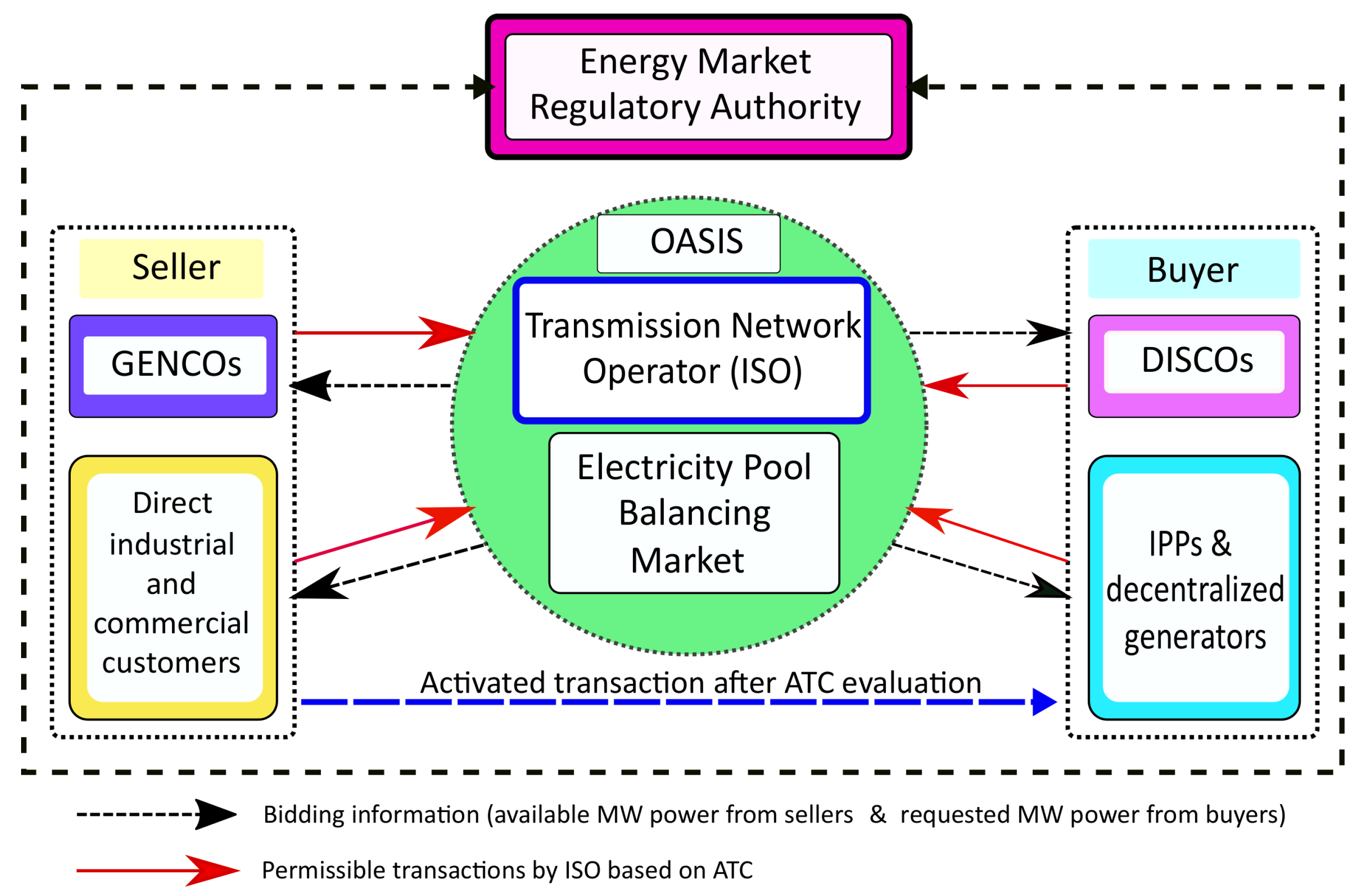
With power system deregulation comes the introduction of energy auction market and hourly energy bidding in real-time power system operation [18]. The market players are connected to the power system control hub to place bids and enter into energy delivery contracts under the monitoring of the ISO, who acts as the transaction evaluator. The information of a specified amount of electrical power (in MW) at a known price will be supply by power producers (generation companies, GENCOs) and the power auctioneer (ISO) will match it with the bids of qualified customers (distribution companies, DISCOs) based on the information they have on their energy management system. In order to prevent power system congestion, the approval of any transaction between a GENCO and a DISCO is subject to the available transfer capability of the grid. Hence, to avoid system overload the ATC is updated regularly on the ISO open access same-time (real-time) information system (OASIS) for all market participants to check and validate the security of their planned transactions as illustrated in Figure 1 [6].

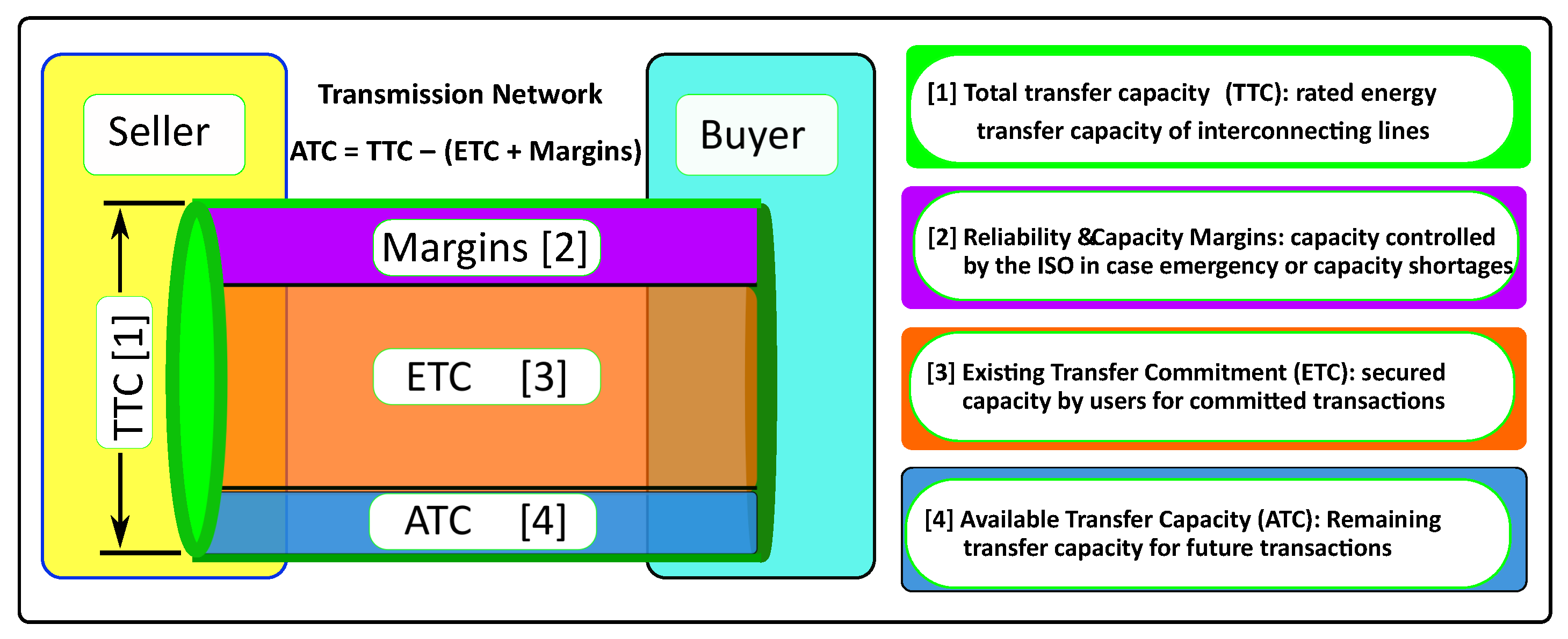
For an economic and reliable supply of electricity, long distance transmission is necessary, especially for inter-area power transactions. The available transmission infrastructure is used by multiple generations and load entities under the competitive bilateral or multilateral transactions [19]. Hence, the ability to allocate a sufficient MW power on transmission lines without violating system’s stability condition is so crucial to the safe and reliable operation of modern power systems. The ATC gives a physical interpretation of these crucial transmission network bottleneck. The ATC is the measure of the yet to be utilized transfer capability of the transmission network which places a limit on the possible amount of additional generation and load increase. It is always calculated as the estimate of the available transmission capacity that will keep the power system within the safe techno-economic operation zones at the nearest future; with adequate consideration for current commercial uses/commitments of the grid facility [20]. Hence, ATC can be calculated as the total transmission capacity less the sum of the ISO-controlled operation margins and the sum of the exiting transmission commitments based on already activated transactions, as illustrated in Figure 2.

Lots of existing research publications have reported the calculation of ATC using several approaches. The commonly adopted approach involves the estimation of some sensitivity factors based on the steady-state operating condition of the power system [21]. The sensitivity factors approach is recognized as being easier and time-efficient. The sensitivity factor gives the relationship between the quantity of active power transaction between two or more buses and the actual power flow along each line. This index is often referred to as the power transfer distribution factor, PTDF. It can either be calculated approximately by using DC power flow as DCPTDF or more accurately using the AC power flow as ACPTDF [22,23]. In this work, the calculation of the ATC for strategic inter-area bilateral transactions is assessed using the voltage stability-based AC-OPF approach.

The performance of the power system in steady-state operating condition based on Newton-Raphson power flow solution is represented by the Jacobian matrix connection between the change in bus power and voltage parameters as given below [24]:

$$\begin{array}{c}\hfill \left[\begin{array}{c}\Delta \delta \\ \Delta V\end{array}\right]={\left[J_T\right]}^{-1}\left[\begin{array}{c}\Delta P\\ \Delta Q\end{array}\right]\end{array}$$

(1)

where the matrix $J_T$ is the Jacobian matrix as described below:

$$J_T=\left[\begin{array}{cc}\frac{\partial P}{\partial \delta }& \frac{\partial P}{\partial V}\\ \frac{\partial Q}{\partial \delta }& \frac{\partial Q}{\partial V}\end{array}\right]$$

(2)

The MW power flow along the transmission line connecting buses i and k in polar form and rectangular form can be written as Equations (3) and (4), respectively:

$$\begin{array}{c}\hfill P_{ik}=V_i{V}_k{Y}_{ik}cos({\theta }_{ik}+{\delta }_k-{\delta }_i)-V_i^2{Y}_{ik}cos{\theta }_{ik}\end{array}$$

(3)

$$\begin{array}{c}\hfill P_{ik}=V_i^2{G}_{ik}-V_i{V}_k{G}_{ik}cos{\delta }_{ik}-V_i{V}_k{B}_{ik}sin{\delta }_{ik}\end{array}$$

(4)

where, $Y_{ik}$ and ${\theta }_{ik}$ are the magnitude and angle of the element in the ith row and kth column of the admittance bus/matrix, $Y_{bus}$. $G_{ik}$ and $B_{ik}$ are the corresponding real part (conductance) and imaginary part (susceptance), respectively. The Taylor’s series expansion (neglecting the higher order terms) of the change (sensitivity dynamics) in active power flow along the line connecting buses i and k, for any inter-bus power delivery, is obtained as:

$$\Delta P_{ik}=\frac{\partial P_{ik}}{\partial {\delta }_i}\Delta {\delta }_i+\frac{\partial P_{ik}}{\partial {\delta }_k}\Delta {\delta }_k+\frac{\partial P_{ik}}{\partial V_i}\Delta V_i+\frac{\partial P_{ik}}{\partial V_k}\Delta V_k$$

(5)

Equation (5) can be re-written in compact matrix form as given below:

$$\Delta P_{ik}=\left[\frac{\partial P_{ik}}{\partial {\delta }_i}\cdots \frac{\partial P_{ik}}{\partial {\delta }_k},\frac{\partial P_{ik}}{\partial V_i}\cdots \frac{\partial P_{ik}}{\partial V_k}\right]\left[\begin{array}{c}\Delta {\delta }_i\\ ⋮\\ \Delta {\delta }_k\\ \Delta V_i\\ ⋮\\ \Delta V_k\end{array}\right]$$

(6)

The sensitivity coefficients in Equations (5) and (6) are obtained from the partial derivative of Equation (4) as defined below [23]:

$$\begin{array}{c}\hfill \frac{\partial P_{ik}}{\partial {\delta }_i}=V_i{V}_k{Y}_{ik}sin({\theta }_{ik}+{\delta }_k-{\delta }_i)\end{array}$$

(7)

$$\begin{array}{c}\hfill \frac{\partial P_{ik}}{\partial {\delta }_k}=-V_i{V}_k{Y}_{ik}sin({\theta }_{ik}+{\delta }_k-{\delta }_i)\end{array}$$

(8)

$$\begin{array}{c}\hfill \frac{\partial P_{ik}}{\partial V_i}=V_k{Y}_{ik}cos({\theta }_{ik}+{\delta }_k-{\delta }_i)-2V_i{Y}_{ik}cos{\theta }_{ik}\end{array}$$

(9)

$$\begin{array}{c}\hfill \frac{\partial P_{ik}}{\partial V_k}=V_i{Y}_{ik}cos({\theta }_{ik}+{\delta }_k-{\delta }_i)\end{array}$$

(10)

According to Equation (1), Equation (6) can be re-written to capture the actual change in power injection as:

$$\Delta P_{ik}=\left[\frac{\partial P_{ik}}{\partial {\delta }_i}\cdots \frac{\partial P_{ik}}{\partial {\delta }_k},\frac{\partial P_{ik}}{\partial V_i}\cdots \frac{\partial P_{ik}}{\partial V_k}\right]{\left[J\right]}^{-1}\left[\begin{array}{c}\Delta P_i\\ ⋮\\ \Delta P_k\\ \Delta Q_i\\ ⋮\\ \Delta Q_k\end{array}\right]$$

(11)

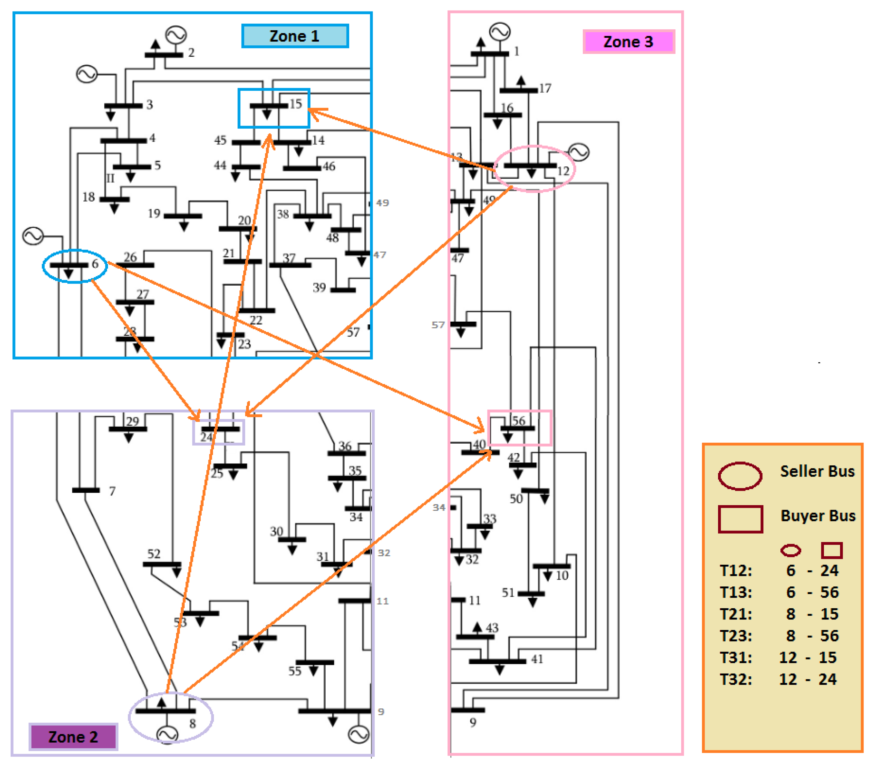
The row vector that contains the sensitivity coefficients is actually sparsely filled with all the coefficients strategically positioned based on the considered line and the total number of load buses [6]. The same situation is realized with the column vector that contains the change in power; for a bilateral transaction between a seller bus p and a buyer bus q, the portion of the transacted power is carried by line connecting any two buses i and k. For a change in MW transaction, $\Delta P_{BTr}$, between transacting buses, the change in the MW flow on the line connecting buses i and k is $\Delta P_{ik}$ and the change in injected power at all buses except the two transacting buses is zero. The change in injected power at buses p and q becomes $+\Delta P_{BTr}$ and $-\Delta P_{BTr}$, respectively.

$$\Delta P_p=+\Delta P_{BTr};\Delta P_q=-\Delta P_{BTr}$$

(12)

This new power mismatch is taken into consideration in Equation (1), for calculating the new system’s operating states from which the change in the power flow in each transmission lines, $\Delta P_{ik}$ can be calculated. Hence, the corresponding AC power transfer distribution factor, $ACPTDF$ for each of the transmission lines is calculated according to Equation (13) [25]:

$$ACPTD{F}_{ik-pq}=\frac{\Delta P_{ik}}{\Delta P_{BTr}}$$

(13)

To compute the $ATC$ from the estimated $ACPTDF$, we first find the maximum allowable MW power flow along all the transmission lines considering their thermal limits and the base case power flow as given below:

$$P_{ik-pq}=\left\{\begin{array}{cc}{P}_{ik}^{max}-P_{ik};& ACPTD{F}_{ik-pq}>0\\ \infty ;& ACPTD{F}_{ik-pq}=0\\ -P_{ik}^{max}-P_{ik};& ACPTD{F}_{ik-pq}<0\end{array}\right\}$$

(14)

where $P_{ik}^{max}$ and $P_{ik}$ are line flow limit and MW power flow along each line for the change in transaction $\Delta P_{BTr}$. Finally, the $ATC$ is specified as the minimum $P_{ik-pq}$ and the corresponding line is the limiting transmission line. The ATC is to be maximized according to Equation (15).

$$\mathrm{maximize}(AT{C}_{pq}=min\left\{\begin{array}{c}{P}_{ik-pq}\end{array}\right\};\forall i,k\in n_b)$$

(15)

3. Voltage Stability Margin Calculation Using Critical Boundary Concept

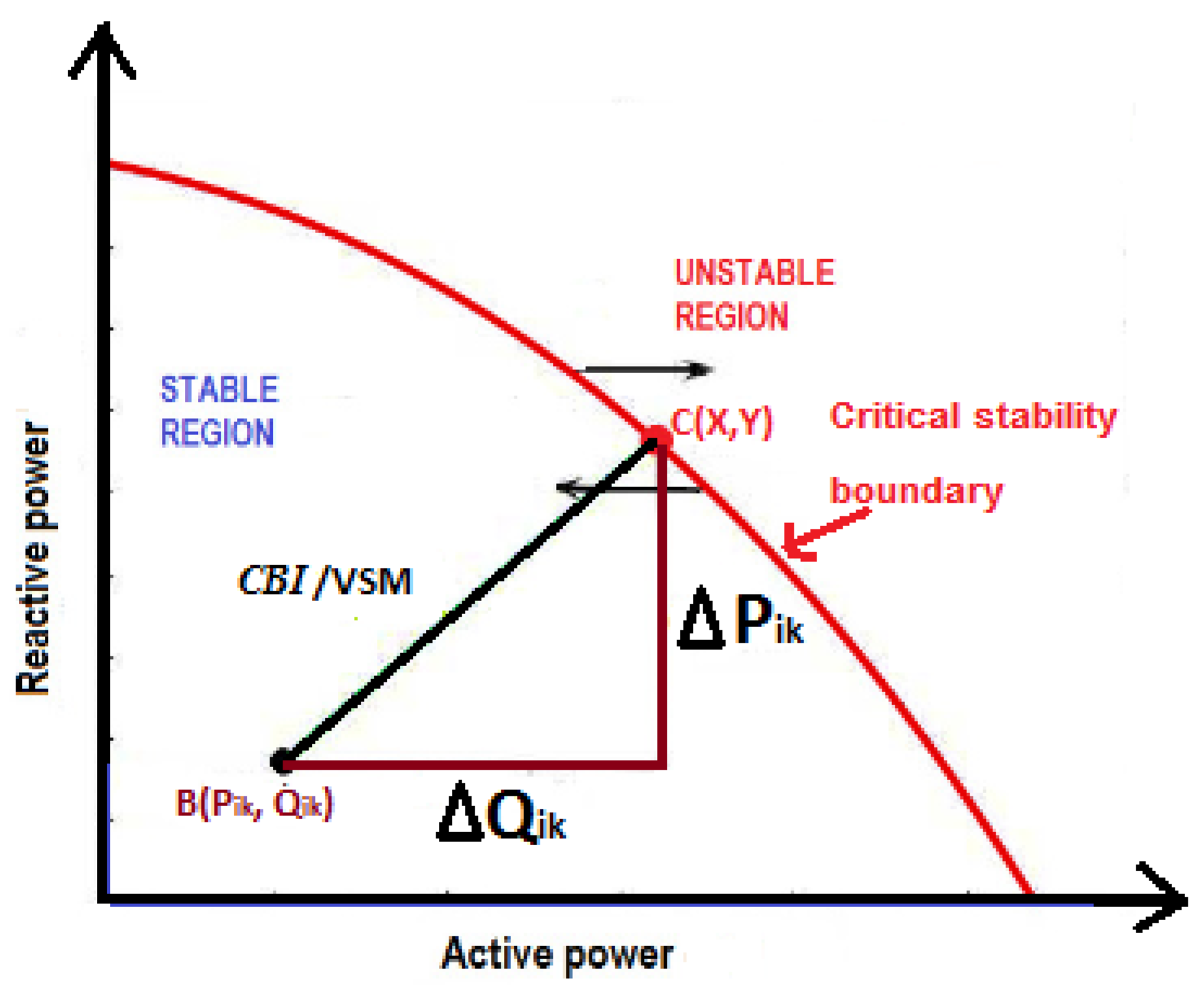
The VSM calculation approach that is used in this study is expressed in terms of the maximum load increase that each transmission line can withstand without violating the system stability limits as illustrated in Figure 3. The details of this optimal stability margin calculation approach are discussed in [26]. The limit for voltage stability of the power system steady-state operation is the boundary curve whose locus is described by Equation (16).

$$\begin{array}{c}\hfill \begin{array}{c}C(X,Y)={\left(r_{ik}X+x_{ik}Y-\frac{V_i^2}{2}\right)}^2-\left(r_{ik}^2+x_{ik}^2\right)\left(X^2+Y^2\right).\hfill \end{array}\end{array}$$

(16)

The VSM, also called the critical boundary index (CBI), is a function of the active and reactive loading as illustrated in Figure 3 and can be obtained by the simultaneous solution of the set of equations obtained from the partial derivatives of Equation (17) with respect to X, Y and $\lambda$:

$$F(X,Y,\lambda )=[{\left(X-P_{ik}\right)}^2+{\left(Y-Q_{ik}\right)}^2]-\lambda C(X,Y)$$

(17)

X and Y are the critical active and reactive loading points, which are nearest to the voltage collapse point, respectively and $\lambda$ is the Lagrangian multiplier for incorporating the stability constraint. The distance between the current operating point, $B(P_{ik},Q_{ik})$ to the point, $C(X,Y)$ on the static critical boundary is calculated and the minimum CBI value (for the most critical line) is to be maximized according to Equation (21).

$$\begin{array}{c}\hfill \Delta P_{ik}=X-P_{ik}^{*}\end{array}$$

(18)

$$\begin{array}{c}\hfill \Delta Q_{ik}=Y-Q_{ik}^{*}\end{array}$$

(19)

$$\begin{array}{c}\hfill CB{I}_{ik}=\sqrt{{(\Delta P_{ik})}^2+{(\Delta Q_{ik})}^2}\end{array}$$

(20)

$$\begin{array}{c}\hfill \mathrm{maximize}\left(CB{I}^{min}\right)\end{array}$$

(21)

$\Delta P_{ik}^{*}$ and $\Delta Q_{ik}^{*}$ are the active (MW) and reactive (MVAR) power flow along each transmission line considering the change in transaction $\Delta P_{BTr}$ between the seller bus and buyer bus without violating the voltage stability margin constraint.

4. Proposed VSC-OPF ATC Enhancement Problem Formulation

In this study, combined ATC and voltage stability margin (VSM) maximization is considered as the objective function using weighted sum approach (WSA). WSA as described in [27] involves merging two or more objective functions together to yield a single objective as given by Equation (22) below. If $\overrightarrow{F}\left(\overrightarrow{x}\right)$ consists of n objective functions each with m decision variables, then the multiobjective problem can be defined as finding the vector ${\overrightarrow{x}}^{*}={[x_1^{*},x_2^{*},\dots ,x_m^{*}]}^T$ which minimizes $\overrightarrow{F}\left(\overrightarrow{x}\right)$ as shown:

$$U=\sum _{i=1}^n{\overrightarrow{W}}_i{\overrightarrow{F}}_i\left(\overrightarrow{x}\right)$$

(22)

${\overrightarrow{W}}_i$ contains the scalar weighting components for each objective function. Based on the above described approach, the objective function in this work is thus described as:

$$\mathrm{maximize}(F=w_1·ATC+w_2·CB{I}^{min})$$

(23)

where:

$$\begin{array}{c}\hfill w_1=1.0\end{array}$$

(24)

$$\begin{array}{c}\hfill w_2=\frac{AT{C}_{base}}{CB{I}_{base}^{min}}\end{array}$$

(25)

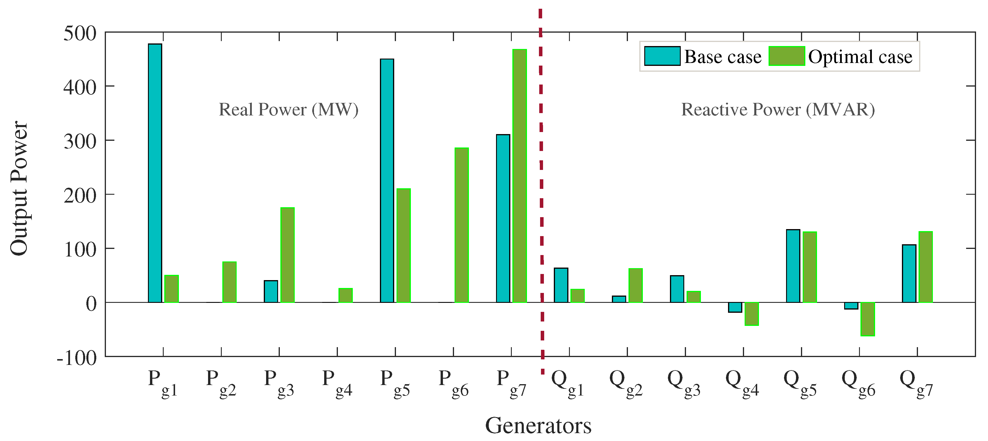
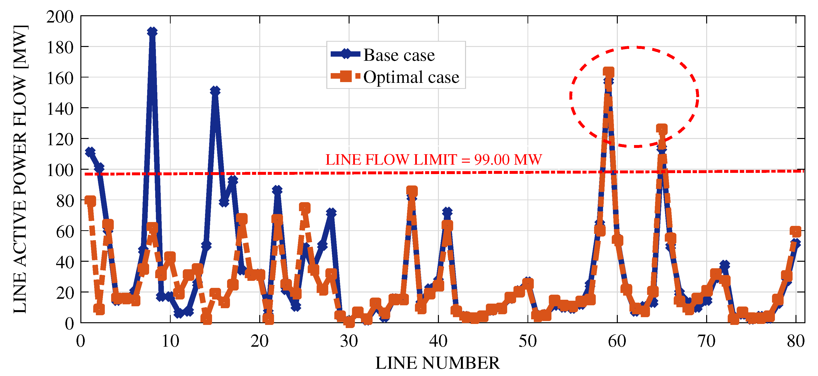
The decision variables are the active and reactive power output, $P_{gen}$ and $Q_{gen}$, of the system generators. $AT{C}_{base}$ and $CB{I}_{base}^{min}$ are the obtained ATC and CBI values at base (non-optimal) case. The system constraints are the power balance equations, generators output ($P_g$ and $Q_g$) limits, bus voltage magnitude (V) limits, line flow limit ($S_L$) and steady-state voltage stability margin ($CBI$) limit as given by Equations (26)–(32) [28,29].

$$\begin{array}{c}\hfill P_{g_i}-P_{d_i}-P_{in{j}_i}=0\forall i;i\in n_b\end{array}$$

(26)

$$\begin{array}{c}\hfill Q_{g_i}-Q_{d_i}-P_{in{j}_i}=0\forall i;i\in n_b\end{array}$$

(27)

$$\begin{array}{c}\hfill P_{g_i}^{min}\le P_{g_i}\le P_{g_i}^{max}\forall i;i\in n_g\end{array}$$

(28)

$$\begin{array}{c}\hfill Q_{g_i}^{min}\le Q_{g_k}\le Q_{g_k}^{max}\forall i;i\in n_g\end{array}$$

(29)

$$\begin{array}{c}\hfill V_i^{min}\le V_i\le V_i^{max}\forall i;i\in n_b\end{array}$$

(30)

$$\begin{array}{c}\hfill |S_{L_{ik}}|\le S_{L_{ik}}^{max}\forall (i,k);(i,k)\in n_b\end{array}$$

(31)

$$\begin{array}{c}\hfill CB{I}_{ik}\ge CB{I}_{ik}^{lim}.\forall (i,k);(i,k)\in n_b\end{array}$$

(32)

Subscript g, d and $inj$ stands for the generation, demand and injected power at each bus. $n_g$ and $n_b$ represents the total number of system generators and buses, respectively. The constraint (minimum limit) of the stability margin of each transmission line is set at 20% of the line’s thermal limit $S_{L_{ik}}^{max}$ [30]:

$$CB{I}_{ik}^{lim}=0.2·S_{L_{ik}}^{max}\forall (i,k);(i,k)\in n_b$$

(33)

The violation of any of the constraints is added to the objective function using the quadratic penalty function approach for constrained optimization [31].

$$F^{*}=F+{\lambda }_{x_i}{(x_i-x_i^{lim})}^2+{\beta }_{u_i}\left(\sum _{i=1}^{N_i}{(u_i-u_i^{lim})}^2\right)$$

(34)

where ${\lambda }_{x_i}$ and ${\beta }_{u_i}$ are the penalty function for the decision variables and parameter limits, respectively. $x_i$ and $u_i$ are the sets of decision variables and constraints.

5. Particle Swarm Optimization Techniques Overview and Variants

PSO algorithm mimicks the behavior of swarm of birds; the behavior of each bird within the swarm is regarded as personal best and the interaction of each bird within the swarm, is considered as global best [32]. The optimal solution is achieved by coordinating the movement of each particle towards its own personal best location, in such a way that the it reinforces the strength of the entire swarm at each generation. The trajectory of each particle is dynamically calculated as the absolute velocity of each particle with reference to its nearest neighbours and the corresponding position in the search space is updated to yield the personal best [33] as illustrated below.

Let: $X_i=[x_{i1},x_{i2},\dots ,x_{id}]$ and $V_i=[v_{i1},v_{i2},\dots ,v_{id}]$, represent the position and velocity vectors of the ith particle in the search space with d-dimension, respectively; the value of the fitness function will be evaluated at each iteration count and the best position of each particle at a particular time (known as the local best) is obtained and stored as $Pbes{t}_i=(p_{i1},p_{i2},\dots ,p_{id})$. The best position out of all the local bests is stored separately as the global best, $Pbes{t}_g=gbest=(p_{g1},p_{g2},\dots ,p_{gd})$. At the succeeding iteration steps, the procedure is repeated, the best out of the local best is selected and compared with the existing global best, if the new best among the local bests performs better it replaces the global best, if not the previous global best is maintained.

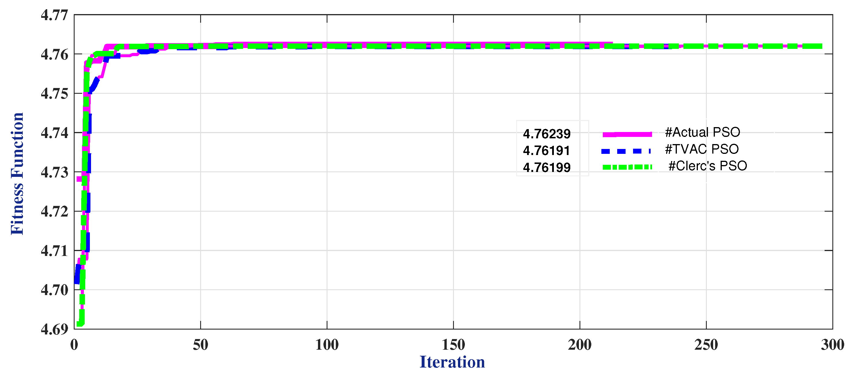
5.1. Classical (Actual) PSO

The velocity and position update dynamics for the fitness function evaluation for a classical PSO are described by Equations (35) and (36):

$$\begin{array}{c}\hfill \begin{array}{cc}\hfill V_{id}^{t+1}& =w·v_{id}^k+c_1·ran{d}_1·(Pbes{t}_{id}-X_{id})\hfill \\ & +c_2·ran{d}_2·(gbes{t}_d-X_{id})\hfill \end{array}\end{array}$$

(35)

$$X_{id}^{k+1}=X_{id}^k+V_{id}^{k+1}$$

(36)

w is the inertia weight that is linearly varying over the generation (iteration).

$$w=(w_f-w_i)·\frac{ite{r}_{max}-iter}{ite{r}_{max}}+w_i$$

(37)

$iter$ is the current iteration count, $ite{r}_{max}$ is the maximum number of iterations. $w_i$ and $w_f$ are the lower and upper boundary values of the inertia weight, respectively. $c_1$ and $c_2$ are the cognitive (personal) and social (global) factors for the swarm interactions, respectively.

5.2. PSO with Time-Varying Acceleration Coefficient (TVAC)

In the classical PSO, $c_1$ and $c_2$ are both chosen to be constant (usually 2.0). However, the social and cognitive factors can be made to be vary linearly with the iteration counts instead of being constant. This is based on a variant of PSO known as PSO with time-varying acceleration coefficients, PSO-TVAC described in [34,35]. This is modelled after the approach of the linearly varying inertia weight as shown below.

$$\begin{array}{c}\hfill c_1=(c_{1f}-c_{1i})·\frac{iter}{ite{r}_{max}}+c_{1i}\end{array}$$

(38)

$$\begin{array}{c}\hfill c_2=(c_{2f}-c_{2i})·\frac{iter}{ite{r}_{max}}+c_{2i}\end{array}$$

(39)

$c_{1i}$, $c_{1f}$, $c_{2i}$ and $c_{2f}$ denotes the start and end limits of the cognitive factor, $c_1$ and the social factor, $c_2$, respectively. The goal is to help to prevent premature convergence and it also helps to achieve better speed of convergence.

5.3. PSO with (Clerc’s) Constricted Weighting Factor

Another PSO convergence improvement approach involves introducing a weighting coefficient, $\chi$ known as the clerc’s constricted factor to the velocity dynamic as defined below [36].

$$\chi =\frac{2}{\left|2-\phi -\sqrt{{\phi }^2-4\phi }\right|}$$

(40)

$$\begin{array}{c}\hfill \begin{array}{cc}\hfill V_{id}^{t+1}& =\chi (w·v_{id}^k+c_1·ran{d}_1·(Pbes{t}_{id}-X_{id})\hfill \\ & +c_2·ran{d}_2·(gbes{t}_d-X_{id}))\hfill \end{array}\end{array}$$

(41)

where ($\phi$ = $c_1$ + $c_2$ and $\phi \ge 4$).

The considered PSO parameters used in this study are provided on

Table 1. PSO Parameters.

Parameter	Values
	Actual PSO	TVAC-PSO	Clerc’s PSO
Population size	150	150	150
Repository Particles	150	150	150
Number of Iterations	300	300	300
Cognitive factor, $C_1$	2.00	2.50–0.50	2.05
Social factor, $C_2$	2.00	0.50–2.50	2.05
Inertia weight, w	0.9–0.4	0.9–0.4	0.9–0.4

.

6. Simulation, Results and Discussion

IEEE 30 and IEEE 57 bus systems are considered as the test cases in this work and the two systems are divided into zones based on available approach in the literature. Several inter-zone bilateral transactions are initiated and the corresponding ATC, CBI and the respective limiting transmission lines are calculated at the base (non-optimal) case. The transaction with the least ATC was selected as the critical transaction for each of the test system. The ATC alongside the CBI are set as the objective function to be maximized using the weighted sum approach as earlier described.

6.1. IEEE 30 Bus System

The result of the ATC calculation for the considered bilateral transactions for IEEE 30 bus system, as shown in Figure 4 is presented in

Table 2. Considered inter-zone bilateral transactions.

Transaction	ATC (MW)	ATC Limiting Line	CBI (MW)	CBI Limiting Line
T1 (2–28)	1.4956	L14 (B6–B28 )	32.97	L37 (B25–B27)
T3 (5–23)	1.5945	L37 (B25–B27)
T2 (13–27)	3.7240	L39 (B27–B30)

. The most critical transactions is T1 (2-28) with the least ATC value of 1.4956 MW and the ATC limiting line is L14 (B6–B28) connecting bus 6 and bus 28. The corresponding minimum CBI for IEEE 30 bus system is calculated as 0.3297 pu (32.97 MW) for CBI limiting line L37 (B25–B27). The optimization procedure is initiated to obtain the simultaneous maximization of the ATC and CBI using the weighted sum approach earlier described. The convergence characteristics of the optimization procedure using the three variants of PSO described in Section 4 is shown in Figure 5 and the analysis of the optimal solution points is presented in

Table 3. Analysis of optimal solution for T1: 2–28.

Variable	Unit	Base	Actual PSO	TVAC-PSO	Clerc’s PSO
$P_{g1}$	MW	98.8705	133.1479	127.9481	130.0155
$P_{g1}$	MW	80.0000	33.7777	46.8005	44.1209
$P_{g1}$	MW	50.0000	40.8118	33.4253	34.0673
$P_{g1}$	MW	20.0000	35.0000	35.0000	35.0000
$P_{g1}$	MW	20.0000	30.0000	30.0000	30.0000
$P_{g1}$	MW	20.0000	16.6168	16.4032	16.3973
$Q_{g1}$	MVAR	18.6928	8.6475	10.1566	9.5948
$Q_{g1}$	MVAR	12.9699	28.2181	24.7707	25.6357
$Q_{g1}$	MVAR	16.4498	19.5664	22.2481	22.0150
$Q_{g1}$	MVAR	21.4739	15.0490	15.1852	15.1750
$Q_{g1}$	MVAR	21.3059	21.4815	21.4976	21.4965
$Q_{g1}$	MVAR	13.5326	13.7317	13.7568	13.7559
$P_{LOSS}$	MW	5.2512	5.3207	5.2574	5.3309
$Q_{LOSS}$	MVAR	19.3021	18.7301	19.0155	18.8952
$V_{min}$	pu	0.9856	0.9832	0.9865	0.9851
$V_{max}$	pu	1.0802	1.0718	1.0668	1.0729
$V_{mean}$	pu	1.0026	1.0013	0.9968	1.0019
ATC	MW	1.4956	1.6894	1.6893	1.6894
CBImin	pu	0.3297	0.3301	0.3300	0.3300

.

The important criteria for comparative analysis of the base (non-optimal) and the optimal cases are the ATC, minimum CBI values (voltage stability margin), the line losses and the voltage profile. The ATC improves from a base value of 1.4956 MW to a value of about 1.69 MW according to the three PSO variants considered. The minimum CBI value, which is the constraining voltage stability margin requirements, improves from the initial value of 0.3297 pu (32.97 MW) to a value of about 0.3300 pu (33.00 MW) for all the considered PSO variants. The line losses are within the same range for both the non-optimal and the optimal cases. There is no significant reduction since line loss minimization is not part of our objective function; however, the fact that there is no outrageous increase in the active and reactive line losses gives more credibility to the optimization problem solved in this work. The voltage profile parameters are consistent with the voltage range for a transmission network set between 0.95 pu minimum and 1.10 pu maximum. The optimal effects on the line flow is shown in Figure 6; the line flows are within the specified line flow limits obtained from the IEEE 30 bus system line data.

One crucial aspect of this work is to ensure the rescheduling of the system generators to ensure an improve system condition for favorable inter-zone transactions and improve system security. Hence, the effect on the ten most critical lines considering VSM is presented in

Table 4. Ten critical lines considering voltage stability limit (CBI) for T1: 2–28.

RANK	Base		Actual PSO		TVAC-PSO		Clerc’s PSO
	CBI [MW]	Line	CBI [MW]	Line	CBI [MW]	Line	CBI [MW]	Line
1	32.97	L39	33.01	L39	33.00	L39	33.00	L39
2	46.02	L41	46.07	L41	46.06	L41	46.06	L41
3	47.31	L13	47.66	L13	47.66	L13	47.66	L13
4	50.49	L38	50.54	L38	50.54	L38	50.54	L38
5	51.29	L36	51.35	L36	51.35	L36	51.35	L36
6	64.15	L40	64.22	L40	64.21	L40	64.21	L40
7	66.95	L35	66.99	L35	66.99	L35	66.99	L35
8	81.35	L34	81.52	L34	81.51	L34	81.51	L34
9	87.72	L26	87.82	L26	87.81	L26	87.81	L26
10	91.29	L23	91.26	L23	91.25	L23	91.25	L23

. The top critical lines (and their corresponding sending end and receiving end buses) are L39 (B27–B30), L41 (B29–B30), L13 (B6–B10), L38 (B27–B29), L36 (B25–B26), L40 (B27–B28), L35 (B24–B25), L34 (B23–B24), L26 (B14–B15) and L23 (B12–B14), respectively. It is observed that there is a credible improvement in the CBI values of each of the lines except for the L23. The reduction is not an aberration since the optimization procedure (with constraints) enforce a power flow re-routing in order to improve the critical portion of the power system.

6.2. IEEE 57 Bus System

The inter-zone bilateral transactions considered for IEEE 57 bus system is shown in Figure 7. The critical transactions, corresponding ATC limiting lines, CBI and CBI limiting line are presented in

Table 5. Considered inter-zone bilateral transactions.

Transaction	ATC (MW)	ATC Limiting Line	CBI (MW)	CBI Limiting Line
T12 (6–24)	0.0118	L62 (B48–B49)	11.36	L36 (B24–B25)
T13 (6–56)	0.0507	L62 (B48–B49)
T21 (8–15)	0.0451	L62 (B48–B49)
T23 (8–56)	0.0306	L62 (B48–B49
T31 (12–15)	0.0529	L62 (B48–B49
T32 (12–24)	0.0099	L62 (B48–B49)

. The most critical transactions is T32 (12–24) with the least ATC value of 0.0099 MW, the ATC limiting line is L62 (B48–B49), and the minimum CBI value is 0.1136 pu (11.36 MW) for the CBI limiting line L36 (B24–B25). The optimization procedure is initiated for the simultaneous maximization of the least ATC and least CBI using the weighted sum approach using TVAC-PSO and the convergence characteristics is shown in Figure 8. The corresponding result for the generator rescheduling is shown in Figure 9. The analysis of the optimal solution point is shown in

Table 6. Analysis of optimal solution point for T32: 12–24.

Variable	Unit	Base	Optimal
$P_{LOSS}$	MW	20.2937	12.1747
$Q_{LOSS}$	MWAR	112.7731	84.9965
$V_{min}$	pu	0.9346	0.9574
$V_{max}$	pu	1.0045	1.0086
$V_{mean}$	pu	1.0016	1.0022
ATC	MW	0.0099	0.0148
CBI	pu	0.1136	0.1244

.

The ATC improves from 0.0099 MW to 0.0148 MW after optimization and the minimum CBI (voltage stability margin) improve from 0.1136 pu (11.36 MW) to 0.1244 pu (12.44 MW) after the optimal generator output rescheduling. There is also a credible reduction in the line losses from 20.2937 MW to 12.1747 MW and 112.7731 MVAR to 84.9965 MVAR for active and reactive power loss, respectively. The line loss reduction translates to credible economic benefit for the system operator since active line loss is directly proportional to cost of operation and reactive line loss is directly proportional to the cost of additional voltage support facilities. The voltage parameters are improved significantly to within the set limit of 0.95 pu minimum and 1.10 pu maximum. The line flow is shown in Figure 10; the active line flow along all the lines are brought within the 99 MW specified limit except for two lines L59 (B14–B46) and L62 (B48–B49). Hence, it yields a credible performance for the transmission line flow and this can be improved upon with the selection of better optimization parameter and fine-tuning. The voltage stability margin as monitored using the critical boundary index improved for all the ten most critical lines i.e., L36(B24–B25), L35(B24–B25), L76(B39–B57), L73(B40–B56), L46(B32–B34), L44(B31–B32), L29(B18–B19), L31(B20–B21), L74(B41–B56) and L43(B30–B31) as depicted in

Table 7. Ten critical lines considering CBI ranking for T32: 12–24.

RANK	Base		Optimal
	CBI [MW]	Line	CBI [MW]	Line
1	0.1136	L36	0.1244	L36
2	0.1229	L35	0.1339	L35
3	0.1723	L76	0.1805	L76
4	0.2039	L73	0.2137	L73
5	0.2233	L46	0.2356	L46
6	0.2280	L44	0.2382	L44
7	0.2759	L29	0.2891	L29
8	0.2802	L31	0.2916	L31
9	0.2966	L74	0.3080	L74
10	0.3512	L43	0.3709	L43

.

7. Conclusions

Voltage stability analysis remains a critical aspect of power system operation and control due to the enormous economical and technical challenges that the collapse of power system can cause. Voltage stability margin can limit the available transfer capacity of transmission network for energy transactions within the power system. Hence, in a bid to maximize profit, curtail grid transfer capacity wastage and ensure overall safety of the power system, output of each of the system’s generators can be constrained-ly rescheduled to ensure that a sufficient voltage stability margin of the power system is maintained. This will have a credible effect on the overall transfer capacity of the power system under bilateral and multilateral energy transactions between the energy producer and buyers. In this work, a voltage-stability constrained optimal power flow (VSC-OPF) problem that involves the joint maximization of available transfer capacity and voltage stability margin for strategically selected bilateral transactions has been investigated. The IEEE 30 bus and IEEE 57 bus systems are used as the test systems and the weighted sum approach is used to achieve a single objective function that was solved using the particle swarm optimization algorithm. From the simulation results obtained, we can conclude that the formulated VSC-OPF approach is sufficient to maintain safe operation and utilization of existing transmission facilities under the considered bilateral transactions. However, the real-time deployment of this approach is limited by the computational time requirement which is comparatively high due to the mathematical procedures involved; thus, the above discussed methodology is more suitable for offline power system security analysis and planning.

References

1. Zhao, J.; Lo, K.L.; Lu, J. Variously worldwide types of deregulated electricity markets and their respective transmission congestion management schemes. In Proceedings of the 2016 51st International Universities Power Engineering Conference (UPEC), Coimbra, Portugal, 6–9 September 2016; pp. 1–6. [Google Scholar] [CrossRef]
2. Ahmadi, M.; Lotfy, M.E.; Shigenobu, R.; Howlader, A.M.; Senjyu, T. Optimal Sizing of Multiple Renewable Energy Resources and PV Inverter Reactive Power Control Encompassing Environmental, Technical, and Economic Issues. IEEE Syst. J. 2019, 13, 3026–3037. [Google Scholar] [CrossRef]
3. Monti, A.; Ponci, F. Electric power systems. In Intelligent Monitoring, Control, and Security of Critical Infrastructure Systems, 1st ed.; Kyriakides, E., Polycarpou, M., Eds.; Springer: Berlin/Heidelberg, Germany, 2015. [Google Scholar]
4. Clements, A.; Hurn, A.; Li, Z. Strategic bidding and rebidding in electricity markets. Energy Econ. 2016, 59, 24–36. [Google Scholar] [CrossRef]
5. Cutsem, T.V.; Vournas, C. Voltage Stability of Electric Power Systems, 3rd ed.; Kluver: Norwell, MA, USA, 2003. [Google Scholar]
6. Gupta, S.K. Power System Operation Control and Restructuring, 1st ed.; I.K. I K International Publishing House: New Delhi, India, 2015. [Google Scholar]
7. Leonardi, B.; Ajjarapu, V. An approach for real time voltage stability margin control via reactive power reserve sensitivities. IEEE Trans. Power Syst. 2013, 28, 615–625. [Google Scholar] [CrossRef]
8. Taylor, C.W. Power System Voltage Stability, 1st ed.; McGraw-Hill: Palo Alto, CA, USA, 1994. [Google Scholar]
9. Seifi, H.; Sepasian, M.S. Electric Power System Planning: Issues, Algorithms and Solutions, 1st ed.; Springer: Berlin/Heidelberg, Germany, 2011. [Google Scholar] [CrossRef]
10. Frank, S.; Rebennack, S. An introduction to optimal power flow: Theory, formulation, and examples. IIE Trans. 2016, 48, 1172–1197. [Google Scholar] [CrossRef]
11. Bhaskar, M.A.; Jimoh, A.A. Available transfer capability calculation using PTDF and implementation of optimal power flow in power markets. In Proceedings of the 2016 IEEE International Conference on Renewable Energy Research and Applications (ICRERA), Birmingham, UK, 20–23 November 2016; pp. 219–223. [Google Scholar] [CrossRef]
12. Manikandan, B.V.; Raja, C.; Venkatesh, P.; Kannan, P.S. Available Transfer Capability Determination in the Restructured Electricity Market. Electr. Power Components Syst. 2008, 36, 941–959. [Google Scholar] [CrossRef]
13. Glazunova, A.M.; Aksaeva, E.S. Available transfer capability determination on the basis of a trade-off approach. In Proceedings of the 2017 IEEE Manchester PowerTech, Manchester, UK, 18–22 June 2017; pp. 1–6. [Google Scholar] [CrossRef]
14. Kumar, A.; Srivastava, S.C.; Singh, S.N. Available transfer capability assessment in a competitive electricity market using a bifurcation approach. IEE Proc. Gener. Transm. Distrib. 2004, 151, 133–140. [Google Scholar] [CrossRef]
15. Othman, M.; Mohamed, A.; Hussain, A. Available transfer capability assessment using evolutionary programming based capacity benefit margin. Int. J. Electr. Power Energy Syst. 2006, 28, 166–176. [Google Scholar] [CrossRef]
16. Abido, M. Optimal power flow using particle swarm optimization. Int. J. Electr. Power Energy Syst. 2002, 24, 563–571. [Google Scholar] [CrossRef]
17. Farahmand, H.; Rashidinejad, M.; Mousavi, A.; Gharaveisi, A.; Irving, M.; Taylor, G. Hybrid Mutation Particle Swarm Optimisation method for Available Transfer Capability enhancement. Int. J. Electr. Power Energy Syst. 2012, 42, 240–249. [Google Scholar] [CrossRef]
18. Karthikeyan, S.P.; Raglend, I.J.; Kothari, D. A review on market power in deregulated electricity market. Int. J. Electr. Power Energy Syst. 2013, 48, 139–147. [Google Scholar] [CrossRef]
19. Rubin, O.D.; Babcock, B.A. A novel approach for modeling deregulated electricity markets. Energy Policy 2011, 39, 2711–2721. [Google Scholar] [CrossRef]
20. Nireekshana, T.; Rao, G.K.; Raju, S.S.N. Enhancement of ATC with FACTS devices using Real-code Genetic Algorithm. Int. J. Electr. Power Energy Syst. 2012, 43, 1276–1284. [Google Scholar] [CrossRef]
21. Mohammed, O.O.; Mustafa, M.W.; Mohammed, D.S.S.; Otuoze, A.O. Available transfer capability calculation methods: A comprehensive review. Int. Trans. Electr. Energy Syst. 2019, 29, e2846. [Google Scholar] [CrossRef]
22. Venkatesh, P.; Gnanadass, R.; Prasad Padhy, D. Available Transfer Capability Determination Using Power Transfer Distribution Factors. Int. J. Emerg. Electr. Power Syst. 2004, 1. [Google Scholar] [CrossRef]
23. Hojabri, M.; Hizam, H. Available Transfer Capability Calculation. In Applications of MATLAB in Science and Engineering, 1st ed.; Michatowski, T., Ed.; IntechOpen: London, UK, 2011. [Google Scholar]
24. Adewuyi, O.B.; Shigenobu, R.; Senjyu, T.; Lotfy, M.E.; Howlader, A.M. Multiobjective mix generation planning considering utility-scale solar PV system and voltage stability: Nigerian case study. Electr. Power Syst. Res. 2019, 168, 269–282. [Google Scholar] [CrossRef]
25. Rao, M.V.; Sivanagaraju, S.; Suresh, C.V. Available transfer capability evaluation and enhancement using various FACTS controllers: Special focus on system security. Ain Shams Eng. J. 2016, 7, 191–207. [Google Scholar] [CrossRef]
26. Furukakoi, M.; Adewuyi, O.B.; Danish, M.S.S.; Howlader, A.M.; Senjyu, T.; Funabashi, T. Critical Boundary Index (CBI) Based on Active and Reactive Power Deviations. Int. J. Electr. Power Energy Syst. 2018, 100, 50–57. [Google Scholar] [CrossRef]
27. Marler, R.T.; Arora, J.S. The weighted sum method for multi-objective optimization: New insights. Struct. Multidiscip. Optim. 2010, 41, 853–862. [Google Scholar] [CrossRef]
28. Adewuyi, O.B.; Lotfy, M.E.; Akinloye, B.O.; Howlader, H.O.R.; Senjyu, T.; Narayanan, K. Security-constrained optimal utility-scale solar PV investment planning for weak grids: Short reviews and techno-economic analysis. Appl. Energy 2019, 245, 16–30. [Google Scholar] [CrossRef]
29. Ahmadi, M.; Lotfy, M.; Howlader, A.; Yona, A.; Senjyu, T. Centralized Multi-Objective Integration of Wind Farm and Battery Energy Storage System in Real Distribution Network Considering Environmental, Technical and Economic Perspective. IET Gener. Transm. Distrib. 2019, 13, 5207–5217. [Google Scholar] [CrossRef]
30. Power Delivery Consultants, Inc. What Limits Power Flow Through an Overhead Transmission Line? Power Delivery Consultants, Inc.: Ballston Lake, NY, USA, 2013. [Google Scholar]
31. McDonnell, J.R.; Reynolds, R.G.; Fogel, D.B. A Survey of Constraint Handling Techniques in Evolutionary Computation Methods. Evol. Program. 1995, 4, 135–155. [Google Scholar]
32. Clerc, M.; Kennedy, J. The particle swarm-explosion, stability, and convergence in a multidimensional complex space. IEEE Trans. Evol. Comput. 2002, 6, 58–73. [Google Scholar] [CrossRef]
33. Valle, Y.D.; Venayagamoorthy, G.K.; Mohagheghi, S.; Hernandez, J.C.; Harley, R.G. Particle swarm optimization: Basic concepts, variants and applications in power systems. IEEE Trans. Evol. Comput. 2008, 12, 171–195. [Google Scholar] [CrossRef]
34. Cui, Z.; Zeng, J.; Yin, Y. An Improved PSO with Time-Varying Accelerator Coefficients. In Proceedings of the 2008 Eighth International Conference on Intelligent Systems Design and Applications, Kaohsiung, Taiwan, 26–28 November 2008; Volume 2, pp. 638–643. [Google Scholar] [CrossRef]
35. Mohammadi-Ivatloo, B.; Rabiee, A.; Soroudi, A.; Ehsan, M. Iteration PSO with time varying acceleration coefficients for solving non-convex economic dispatch problems. Int. J. Electr. Power Energy Syst. 2012, 42, 508–516. [Google Scholar] [CrossRef]
36. Raha, S.; Som, T.; Chakraborty, N. Constriction factor based particle swarm optimization applied to reactive power dispatch in transmission system. In Proceedings of the International Conference on Sustainable Energy and Intelligent Systems (SEISCON 2011), Chennai, India, 20–22 July 2011; pp. 335–339. [Google Scholar] [CrossRef]
37. Bhuyan, S.; Hazarika, S.; Bardalai, A. Power flow analysis on IEEE 57 bus system using MATLAB. Int. J. Eng. Res. Technol. 2014, 3, 1161–1171. [Google Scholar]
Figure 1. Deregulated electricity market.
Energies 12 04371 g001
Figure 2. Illustration and basic estimation of ATC.
Energies 12 04371 g002
Figure 3. P-Q curve showing the transmission line voltage stability margin.
Energies 12 04371 g003
Figure 4. IEEE 30-Single line diagram and investigated inter-zone transactions [23].
Energies 12 04371 g004
Figure 5. Convergence characteristics for T1: 2–28.
Energies 12 04371 g005
Figure 6. Line power flow for T1:2–28.
Energies 12 04371 g006
Figure 7. IEEE 57-Single line diagram and investigated inter-zone transactions [37].
Energies 12 04371 g007
Figure 8. IEEE 57-Convergence characteristics for T32: 12–24.
Energies 12 04371 g008
Figure 9. IEEE 57-System generators’ outputs for T32: 12–24.
Energies 12 04371 g009
Figure 10. IEEE 57-Line power flow for T32: 12–24.
Energies 12 04371 g010