Abstract
In the paper, a modified coyote optimization algorithm (MCOA) is proposed for finding highly effective solutions for the optimal power flow (OPF) problem. In the OPF problem, total active power losses in all transmission lines and total electric generation cost of all available thermal units are considered to be reduced as much as possible meanwhile all constraints of transmission power systems such as generation and voltage limits of generators, generation limits of capacitors, secondary voltage limits of transformers, and limit of transmission lines are required to be exactly satisfied. MCOA is an improved version of the original coyote optimization algorithm (OCOA) with two modifications in two new solution generation techniques and one modification in the solution exchange technique. As compared to OCOA, the proposed MCOA has high contributions as follows: (i) finding more promising optimal solutions with a faster manner, (ii) shortening computation steps, and (iii) reaching higher success rate. Three IEEE transmission power networks are used for comparing MCOA with OCOA and other existing conventional methods, improved versions of these conventional methods, and hybrid methods. About the constraint handling ability, the success rate of MCOA is, respectively, 100%, 96%, and 52% meanwhile those of OCOA is, respectively, 88%, 74%, and 16%. About the obtained solutions, the improvement level of MCOA over OCOA can be up to 30.21% whereas the improvement level over other existing methods is up to 43.88%. Furthermore, these two methods are also executed for determining the best location of a photovoltaic system (PVS) with rated power of 2.0 MW in an IEEE 30-bus system. As a result, MCOA can reduce fuel cost and power loss by 0.5% and 24.36%. Therefore, MCOA can be recommended to be a powerful method for optimal power flow study on transmission power networks with considering the presence of renewable energies.
1. Introduction
Optimal power flow (OPF) is a very important optimization problem in power system operation due to its huge contribution to economy and stable operation issues. The task in the problem is to determine the most appropriate values for parameters of electric components in transmission power networks so that all operation limitations of the power system are always in the allowable ranges and predetermined objectives are also optimized [1,2]. Basically, single objective functions considered in the OPF problem are fuel cost of generators, power losses of all branches, deviation of load voltage, and index of voltage stability while taking into account operation constraints of all components such as active and reactive power output limitations of generators, tap limitation of transformers, reactive power output limitations of switchable capacitor banks, load bus voltage limitations, and transmission line capacity limits. In the OPF problem, there are many parameters corresponding to working parameters of electric components in transmission power networks. The parameters are divided into two variable types, control variables and dependent variables. The former includes active power of generators excluding the generator with the highest capacity located at the slack bus, voltage of generators, reactive power generation of shunt capacitors, and tap position of transformers. The latter includes other remaining parameters such as active power of the generator located at the slack bus, reactive power of generators, apparent power of all conductors, and voltage of all load buses. In summary, the key work in the OPF problem is to select control parameters of power networks in order to satisfy all constraints and optimize predetermined objectives.
In the past, the mathematical model of the OPF problem did not consider non-differentiable objectives as well as complicated constraints of generators. Therefore, the OPF problem was easily solved by conventional deterministic optimization algorithms, which were mainly based on derivatives and gradient techniques. Nowadays, the OPF problem becomes a complex problem under considering non-convex or non-smooth objectives, and a high number of branches and generators. Therefore, the applications of the deterministic optimization algorithms must be stopped and replaced with other powerful algorithms. This issue boosts big motivations from researchers to propose new methods with the main purpose of tackling such shortcomings. Metaheuristic algorithms comprising of standard methods, improved methods, and hybrid methods were applied for coping with the OPF problem. Modified evolutionary programming (MEP) has been proposed for solving the OPF problem [3]. MEP was the combination of conventional evolutionary programming (EP) and conventional simulated annealing algorithm (SA). In the method, the mutation technique was established by using both Gaussian and Cauchy distributions whilst the selection technique was done by using the probabilistic updating technique of SA. MEP was compared to EP in solving the IEEE 30-bus transmission power network. Fuel cost comparison indicated that MEP was more effective than EP in terms of the optimal solution. However, MEP had a longer execution time, although the two methods have been run by setting the same values for population size and the number of iterations. Differential evolution variants, such as conventional differential evolution (DE) [4,5], differential evolution with augmented Lagrange multiplier method (DE-ALM) [6], improved differential evolution (IDE) [7,8], were employed for dealing with OPF problem. In [4], the search ability of DE has been tested on the OPF problem with two power systems considering single objective function and multi-objective function. In addition, the Grey Wolf algorithm has been implemented for the same study cases with the intent to demonstrate the high performance of DE for the OPF problem. DE has been evaluated to be more effective than GWOA and other existing methods such as PSO, TLO, and GSA; however, the authors have forgot convergence speed comparison, which is the most important factor for leading the conclusion of real performance. As reported in [4], both DE and GWOA were run by setting 300 and 1000 to the highest number of iterations for IEEE 30-bus system and IEEE 118-bus system, but population size was not shown for the two methods. Clearly, the execution of DE was only for good results rather than the demonstration of a high performance of DE. In [5], the authors have also tried to show the effectiveness of DE by running DE on an IEEE 30-bus system with different objective functions. The study has set different values for the number of iterations although only the IEEE 30-bus system was the test case. For the case with the good result, the number of iterations was set to 200, but for the case with worse results it was increased to 500 iterations. The settings in [5] obtained good results, but for the demonstration of a real performance of DE. In [6], the authors have stated DE was not effective for the OPF problem because mutation factor was set to a fixed value and its ability for handling inequality constraint was not highly effective. Therefore, in DE-ALM, mutation factor and crossover factor have been considered as control variables. Additionally, augmented Lagrange multiplier method (ALM) was applied for dealing with inequality constraints. DE-ALM has been compared to other metaheuristic algorithms but the comparisons with DE have been ignored. Clearly, the proposed modifications in [6] could not lead to any conclusions of the improved performance of DE-ALM. In contrast with DE-ALM, IDE methods [7,8] have only focused on improvements of mutation stage by employing dissimilar models for updated step size. In [7], IDE and conventional DE have been tested on IEEE 6-bus and IEEE 30-bus systems for comparisons. In [8], larger systems with 30 buses and 57 buses have been used as study cases for proving the effectiveness of IDE. The two studies in [7,8] have focused on the minimum fitness function but ignored the comparison of population size and the maximum iterations. Therefore, the conclusion of high performance of IDE was not persuasive. In addition to DE variants, particle swarm optimization (PSO) variants were also successfully applied for the OPF problem considering different objectives and complicated constraints. These methods consist of PSO with chaos queues and self-adaptive mechanisms (IPSO) [9], evolving ant direction particle swarm optimization (EADPSO) [10], PSO with Pseudo-Gradient theory (PG-PSO) [11], graphics processing unit based PSO (GPUA-PSO) [12], and PSO with canonical differential evolution (CDE-PSO) [13]. In [9], the authors proved the outstanding performance of IPSO over conventional PSO through an IEEE 30-bus system considering multi-objective function. These authors have found a set of non-dominated solutions and chosen one out of the solutions to be the best compromise solution. There was no report of control parameters for search speed comparison. The shortcoming in [9] was tackled in [10] since the demonstration of search speed was carried out. EADPSO and PSO have been run in the same setting of control parameters and in different settings for further comparisons. However, the study cases were two systems with 39 buses and 57 buses. Furthermore, the comparisons between EADPSO and previous methods were carried out based on objective functions only. Among these methods, PG-PSO in [11] was the most promising optimization tool thanks to the applications of the pseudo-gradient approach and constriction factor. In PG-PSO, pseudo-gradient was in charge of finding the best direction for each particle in order to speed up its convergence process. In addition, the constriction factor could support finding a reasonable distance between the old solution and new solution. Via the test results from benchmark functions and standard IEEE transmission power networks with 14, 30, 57, and 118 buses, the proposed method has been stated to be more effective than the conventional PSO. The studies in [12,13] have also tried to prove the real effectiveness of the applied methods by showing less fuel cost and less total power loss than other methods; however, the setting of iterations has not been considered for comparisons. In fact, the number of iterations was set to 3000 in [12] and 1000 in [13] for an IEEE 30-bus system whereas the settings for other remaining systems were not reported. Aside from DE and PSO variants, genetic algorithm (GA) variants were thoroughly exploited for the OPF problem by testing the conventional genetic algorithm and analyzing its shortcomings. Different modified versions of GA have been employed such as genetic algorithm (GA) with fuzzy system (FS-GA) [14], enhanced GA with new decoupled quadratic load flow (DQLF-EGA) [15], efficient GA with incremental power flow model (EGA-IPL) [16], and efficient GA with boundary method (EGA-BM) [17]. In [14], FS-GA has been compared to GA via three test systems with 6, 26, and 30 buses. The study has demonstrated the real effectiveness of the combination of GA and fuzzy mechanism, but it has ignored the comparison between FS-GA and other methods. In [15], DQLF-EGA and several PSO methods have been implemented for only the IEEE 30-bus system whereas the comparisons with other methods have not been considered. However, both FS-GA and DQLF-EGA have been considered as favorable methods for the OPF problem in [14,15]. In the GA method group, HEGA-BM was the most complicated method because it was created by combining HEGA [16] and a proposed boundary method. The strong point of such method was to solve all violations of upper and lower boundaries of OPF easily and successfully. HEGA-BM has provided better solutions than EGA-IPL for systems with 30 and 118 buses. However, the main limitation in [16] was that the comparisons with other existing methods were few. In fact, just conventional methods like PSO, GA, and DE were compared to HEGA-BM. In addition to above popular methods, a huge number of methods consisting of original methods, improved methods, and hybrid methods have also been suggested to cope with big challenges from the OPF problem [18,19,20,21,22,23,24,25,26,27,28,29,30,31,32,33,34,35,36,37,38]. IHBMO [20] was proposed in 2011 based on the honey bee mating optimization algorithm (HBMO) by using the mutation mechanism. The method could effectively handle some drawbacks of HBMO such as high probability of finding local optima and converging to global optima with long simulation time. Unlikely, ISSO [38] was the latest tool and formed from the social spider optimization (SSO) by suggesting some improvements such as employing a new movement method of female and male spiders and proposing a suitable ratio of female spiders to male spiders. With the use of the proposed improvements, ISSO has found more impressive solutions than SSO and other methods. Among the studies, multi-objective function consisting of two single objectives such as fuel cost and power loss, power loss and voltage deviation, and fuel cost and voltage deviation were considered in [18,19,21,23,24,27,30,33]. The main limitation in the studies was the trade-off between two objectives since one objective was better but another was worse. Furthermore, the set of non-dominated solutions was not high enough to determine the best compromise solution. Almost all methods were run on an IEEE 30-bus system whereas few methods were run on an IEEE 118-bus system. For leading to a conclusion of performance for the multi-objective problem, these studies have only focused on fuel cost, power loss, and voltage deviation but convergence speed reflected via the setting of control parameters. Clearly, the real performance of methods for the OPF problem was not demonstrated persuasively and their key shortcomings were as follows:
- 1
- They have compared a proposed method with other existing methods shown in other studies meanwhile they have forgot to demonstrate the improvement of the proposed method over the standard method.
- 2
- They have compared a proposed method with standard method, but they have forgot to compare the method with other methods.
- 3
- For the studies that compare the proposed method to both standard method and other existing methods, the comparisons were only about objective functions not about convergence speed.
In the paper, we have tackled the disadvantages by comparing the proposed method (MCOA) with the standard method (OCOA) and other existing methods. In addition, the conclusion of real performance of MCOA was established by taking into account the comparison of obtained results and the setting of control parameters.
In recent years, many metaheuristic algorithms have been developed for the purpose of solving complicated optimization problems. Among these methods, original Coyote optimization algorithm (OCOA) in [39] is one of the most interesting methods with strange structure and very high performance as compared to many metaheuristic algorithms. Forty functions with different dimensions corresponding to 92 study cases have been employed to implement OCOA and six popular metaheuristic algorithms such as PSO, ABCA, SOSA, BA, GWOA, and FA. OCOA could improve the result over these six methods significantly once OCOA has found a better average fitness function for many test cases, especially for hybrid benchmark functions with high dimensions, which were representatives of complicated optimization problems. Recently, OCOA has been successfully applied for different optimization problems in these studies [40,41,42,43]. In [40], OCOA has been applied for finding main parameters of three-diode based photovoltaic modules under different environment conditions consisting of the change of temperature and the change of irradiation. Thanks to the high performance of OCOA, the three-diode photovoltaic model could be established and it could work as effectively as other commercial Photovoltaic modules in the market. In [41], OCOA has been applied for reducing gas consumption of turbines in combined cycle power plants in Brazil while satisfying pollutant emission regulations and physical limitations of turbines. OCOA has been evaluated to be more effective than ABCA, BSA, SaDE, GWOA, PSO and the Symbiotic Organisms Search (SOS). In [42], OCOA together with GA and PSO have been implemented for solving the economic dispatch problem with the integration of wind turbines and thermal power plants. The first system with five thermal power plants and one wind turbine and the second system with 10 thermal power plants and two wind turbines have been studied for comparisons. The target of the work was to minimize total cost of thermal power plants and total cost of wind turbines. OCOA has reached less cost than GA and PSO for the two systems. In [43], OCOA was applied for solving the reactive power dispatch problem in power system optimization operation; however, OCOA was less effective than other compared methods since quality of voltage of load buses and total power losses in transmission lines were worse than those of other methods. Although OCOA has been applied successfully for different problems, its real performance is still not demonstrated persuasively. Among the studies in [39,40,41,42,43], only optimal reactive power dispatch problem in [43] is a real challenge for evaluating the effectiveness of OCOA. The result comparisons in [43] indicated that OCOA could not reach good results as other methods, even the success rate of OCOA was very low. As observing results from the first application of OCOA on benchmark function in [39], the most optimal solutions of the considered function set had “zero” value whereas OCOA has used a center solution in the first new solution generation technique. The center solution approximately owns variables with middle point of upper bound and lower bound. Therefore, the center solution is very effective for OCOA in finding new solutions as solving benchmark functions. This regard is completely not effective for the OPF problem. In the second new solution generation technique, OCOA has used three random variables where two ones are taken from two randomly chosen existing solutions and another one is randomly produced within the upper and lower bounds. At the end of each iteration, OCOA performs solution exchange action among available groups. The action is useful for avoiding lumping solutions in each group; however, it cannot happen certainly due to the comparison condition between a random number and a predetermined number. Clearly, randomizations are existing in OCOA. Due to the existing shortcomings of the two new solution generation techniques and the solution exchange technique, OCOA cannot be a promising method for the OPF problem. It cannot find high quality solutions effectively and it must use a high number of computation steps. For avoiding these disadvantages of OCOA, we propose modified coyote optimization algorithm (MCOA) by applying three modifications on the two new solution generation techniques and the solution exchange technique. In the first modification, we suggest replacing the center solution with the best solution. In the second modification, we cancel randomizations of the second technique by searching nearby the best solutions. In the third modification, the action of exchanging solutions among available groups is certainly performed by canceling the comparison condition. Consequently, the proposed modifications can bring the contributions to the proposed MCOA method as follows:
- 1
- The replacement of the center solution is useful in reducing computation steps and shortening simulation time,
- 2
- The replacement of randomizations in the second new solution technique can reduce the negative impact of randomizations and give more chances for finding more promising solutions,
- 3
- Quitting condition of the solution exchange to make certainty of solution exchange among groups. This can avoid all solutions a group falling into local optimal zones and also reduce computation steps.
In order to test the effectiveness and robustness of the proposed MCOA, three IEEE transmission power systems with 30 buses, 57 buses, and 118 buses are utilized as main study cases. The main task of the methods is to determine control parameter of transmission power networks meanwhile the objective is to minimize total fuel cost of all thermal generating units and total power losses in all transmission lines. Furthermore, for the case of the IEEE 30-bus system, one photovoltaic system with rated power of 2.0 MW is proposed to be installed in order to reduce fuel cost of all thermal generating units and power loss in all transmission lines. As comparing obtained results, the main contributions of the study are as follows:
- 1
- MCOA can reach a higher success rate than OCOA as solving the OPF problem, especially for the largest scale system with 118 buses,
- 2
- MCOA can find better optimal solutions than OCOA for all study cases,
- 3
- OCOA and MCOA methods are successfully applied for the OPF problem with the presence of a photovoltaic system,
- 4
- The best site of photovoltaic system (PVS) in the transmission power network found by MCOA can result in much smaller fuel cost and power loss,
- 5
- MCOA is superior to other compared methods.
In addition to the introduction section, the other parts of the paper are organized as follows: the mathematical formulation of OPF problem with the presence of objective functions and power system constraints is given in Section 2. The entire search procedure of OCOA is expressed and then the proposed MCOA is clarified in Section 3. All computation steps of using the proposed MCOA for the OPF problem are described in detail in Section 4. Simulation results and discussion of three IEEE transmission power networks are presented in Section 5. Conclusions are added in Section 6.
2. Mathematical Formulation of the OPF Problem
In this part, the considered OPF problem is expressed in terms of mathematical formulations with the presence of single objective functions and constraints. Two single objectives are considered to be reduction of electric generation cost and reduction of power losses. All constraints in transmission grids must be satisfied such as operating limits of all electric components and power balance at all load buses. The objective functions and constraints are presented in detail as follows.
2.1. Single Objective Functions
2.1.1. Electric Generation Fuel Cost Reduction
In the OPF problem, power sources are thermal power plants using fossil fuels for producing electric and supplying to loads. Therefore, the target of reducing electric generation fuel cost is equivalent to the target of optimizing the generation of all thermal power plants. Basically, thermal power plants’ characteristics are represented as the relationship of power output and electric generation fuel cost. The operating efficiency of these thermal power plants can be evaluated by the total fuel cost for the generated power. The target of reducing fuel cost can be mathematically formulated by the following Equation (1) [5]:
where a1k, a2k, a3k, a4k, a5k are coefficients in electric generation fuel cost function of the kth thermal power plant; EGFCk is the electric generation fuel cost of the kth thermal power plant; NoG is the number of thermal power plants in the considered transmission grid; Pk is the generated power of the kth thermal power plant. In the OPF problem, control variables and dependent variables of each solution are as follows:
where CVari and DVari are the control and dependent variable sets of the ith solution. Corresponding to each variable in the two sets, the definitions are as follows:
- 1
- k = 2, …, NoG for Pk,i,
- 2
- k = 1, …, NoG for Vk,i,
- 3
- t = 1, …, NoT for Tt,i,
- 4
- c = 1, …, NoSVC for SVCc,i,
- 5
- l = 1, …, NoL for VLl,i,
- 6
- k = 1, …, NoG for Qk,i,
- 7
- br = 1, …, NoBR for MVAbr,i.
2.1.2. Total Active Power Losses (TAPL) Reduction
Total power generated by all generators is supplied to loads via transmission lines. With the presence of resistance and reactance, transmission lines cause active and reactive power losses in which active power loss is considered as a major objective in the OPF problem. In fact, the transmission lines account for a high rate in all electric components in the power systems. Therefore, the active power losses in all transmission lines must be optimized as an objective. The objective can be expressed by the mathematical model below [4]:
2.2. Constraints of the OPF Problem
The constraints of the OPF problem are similar to the constraints of control variables and dependent variables together with the constraint of power balance at all buses. The constraint of variables is the limits of electric components in the considered transmission grid such as generator of thermal power plants, static VAR compensator, tap changer of transformers, loads, and transmission branches. Among the components, the generator of thermal power plants is the most complicated due to the consideration of active power, reactive power, and voltage. With respect to mathematical formulation, the constraint of electric components can be expressed in terms of inequalities whereas the constraint of power balance at all load buses can be expressed in terms of equalities. All the constraints are shown as follows.
2.2.1. Constraints of all Electric Components
The generator of thermal power plants is constrained by upper and lower bounds of voltage, active, and reactive power as follows [11]:
In addition, transformers, static VAR compensators, load, and transmission branches are constrained by upper and lower bounds as follows [10]:
2.2.2. Constraints of Active and Reactive Power Balance
Two equality constraints are considered in the considered OPF problem to be the active power balance and the reactive power balance at each bus in the transmission grid. The two constraints are shown as follows [23]:
As seen from the two equalities above, generated power Pj must be equal to the sum of the load demand PLj and the power supplying to the branch connecting bus j and bus i.
In this paper, we consider three benchmark power systems with 30, 57, and 118 buses that have the same characteristics of a real system. In fact, the systems are comprised of transformers, capacitors, conductors, generators, loads, and buses. These components are represented by important parts and included in the OPF problem. For instance, transformers are represented as the tap changer and limitations of the tap changer are considered in Equation (8). Capacitors are also concerned and installed at some buses with the intent to supplement reactive power to loads and control voltage of load buses. Limitations of reactive power from the capacitors are shown in Equation (9). Important parameters of loads are active power, reactive power, and working voltage limitations. Voltage limitations of loads are shown in Equation (10) meanwhile the balances of active and reactive power are shown in Equations (12) and (13). Conductors or transmission lines are taken into account by the presence of apparent power limits shown in Equation (11). In dealing with optimization problems in power systems, the most difficult task is to collect parameters of electric components in real systems. Therefore, the solution is to use these benchmark systems that have the same characteristics of real systems.
3. The Proposed Method
3.1. Original Coyote Optimization Algorithm
OCOA was inspired from the natural behaviors of coyotes. The strange characteristics of OCOA are two new solution generation techniques and one more technique for exchanging solutions among groups. OCOA is totally different from other metaheuristic algorithms since the whole population is divided into a number of groups (NoGr) and there is a number of members in each groups (NoCoy). Each coyote is represented by its social condition and quality of the social condition. Between the two factors, the former is corresponding to the optimal solution and the latter is corresponding to the fitness function value of the optimal solution. OCOA executes two techniques for producing two new solution times. OCOA produces (NoGr × NoCoy) solutions in the first time but OCOA produces NoGr solutions in the second time. It is noted that the result of (NoGr × NoCoy) is also population size. All solutions in each group are newly updated in the first technique while only one solution in each group is newly updated in the second technique. At the last step of OCOA, two randomly picked solutions in two randomly chosen groups can be exchanged based on a predetermined condition. Therefore, it seems to be that OCOA is a promising method for the considered OPF problem. For better understanding of OCOA, the whole computation steps of OCOA method are described in detail as follows [39]:
Similar to other existing meta-heuristic algorithms, the first stage in the search process of OCOA is initialization with the target of producing the initial solutions. Each coyote in each group is a solution of the optimization problem and it is represented as Coym,g where m is the mth coyote in each group and g is the gth group. Each solution is randomly produced based on the following model:
where LB and UB are respectively lower and upper bounds of solutions. In addition, each solution contains NoCV control variables.
Each solution Coym,g is evaluated by calculating fitness function FTm,g and the best solution of each group is determined and set to Coybest,g.
3.2. Two New Solution Generations
Unlike PSO, which has one new solution generation, OCOA is provided with two techniques of generating new solutions for each iteration. Each group produces NoCoy solutions for the first generation but produces only one new solution for the second generation. The first technique is performed by the meaning of the following equation:
In Equation (15), Coym,g on the left hand side is the newly updated solution meanwhile Coym,g on the right hand side is the old solution. In case that Coym,g on the left hand side and Coym,g on the right hand side are the same, it means the solution is not newly updated. However, the possibility of the situation is very low or nearly equal to zero. In order to determine the center solution Coycen,g, one by one variable in the gth group is sorted in descending order of values and then the middle value is selected for the considered variable.
For the second generation, OCOA selects one out of three ways for taking control variables for the sole solution. Each group produces one solution Coyg, which is represented as follows:
where varn,g is determined by the following rule:
where varn,pr1,g and varn,pr2,g are two variables that are taken from the first randomly picked solution and the second randomly picked solution, respectively. If the first condition, , is true, varn,pr1,g is selected but if the second condition, , is true, varn,pr2,g is selected. In the case that both of the conditions are incorrect, varn,rd is randomly produced within the lower and upper bounds.
3.3. Correction of New Solutions
New solutions Coym,g and Coyg in Equations (15) and (16) need verification and correction before evaluating quality. The verification and correction can be carried out by the function of the following models:
3.4. Solution Exchange among Available Groups
OCOA terminates each iteration by performing solution exchange among available groups. However, the action is not always performed and dependent on the condition below:
If the condition in Equation (20) occurs, two randomly picked solutions in two random groups are exchanged together. Otherwise, all solutions are retained in their current position.
3.5. Modified Coyote Optimization Algorithm (MCOA)
3.5.1. The First Proposed Modification
In the first proposed modification, we suggest changing Equation (15) by replacing Coycen,g with CoyGbest and replacing Coypr1,g and Coypr2,g with Coym,g. As a result, all solutions in the gth group are produced by the following formula:
In Equation (21), the center solution was removed due to its negative impacts on the quality of new solutions of the OPF problem. The OCOA in [39] was applied for benchmark optimization functions, meanwhile approximately all functions had an optimal solution with zero values. Thus, the center solution was highly effective for generating updated steps and new solutions for OCOA with benchmark functions. In the paper, optimal solutions of the OPF problem has a set of control variables with different values. For instance, power output of generators is in the range of higher than 0 and can be up to 1000 MW, meanwhile reactive power of static VAR compensators can be up to tens of MVAR. Unlikely, the tap changer of transformers and load bus voltage have values around 1.0 Pu. Consequently, center solutions can negatively influence the performance of OCOA for optimal solutions of the OPF problem. In addition, Equation (21) has employed the old solution Coym,g instead of two randomly picked solutions Coypr1,g and Coypr2,g like Equation (15). The modification can assure that all solutions in the considered group are used to generate updated steps and new solutions.
3.5.2. The Second Proposed Modification
In the second improvement, Equation (17) is suggested to be modified due to its low effectiveness of randomization in producing control variables of the sole new solution. The first control variable is selected by the comparison between a random number and (1/NoCV) while the second control variable is determined based on the comparison between the random number and (1/NoCV + 0.5). If the first two conditions are not met, a random control variable is produced within upper and lower bounds. Clearly, the combination of the three randomizations cannot lead to a good solution with high quality excluding the diversification of generated control variables. For avoiding missing a promising solution, we suggest Equations (16) and (17) should be canceled and replaced with a new one that can support generating a more favorable solution. The new formula is as follows:
3.5.3. The Third Proposed Modification
In the third improvement, we suggest ignoring the comparison condition for exchanging solutions shown in Equation (20). Regarding the review on the action of exchanging solutions among groups, the action can diversify the solutions in each group. Thus, we select two random groups and exchange two randomly picked solutions in the groups.
4. Implementation of the Proposed Method for the OPF Problem
4.1. Population Initialization
OPF is a nonlinear problem with a high number of control variables and it needs to solve the problem simply and easily. In the study, we used the proposed MCOA method to find good control parameters of transmission power networks and then the found control parameters were added into the Matpower program where Newton-Graphson was run to find remaining dependent parameters of transmission power networks consisting of generation of slack bus, voltage of all load buses, reactive power of generators, and branch currents. Each solution of MCOA contains a set of control variables that are parameters in transmission power network such as voltage and active power of generators, working reactive power of compensators, and secondary voltage of transformers. For evaluating the quality of each solution, the sum of the considered objective function and the violation of all dependent parameters is calculated. In the first step, the set of control variables consisting of Pk,i (k = 2, …, NoG), Vk,i (k = 1, …, NoG), Tt,i (t = 1, …, NoT) and SVCc,i (c = 1, …, NoSVC) is randomly produced as follows:
4.2. Solution Quality Evaluation
After determining all control variables as shown in Equations (23)–(26), such control variables are sent to input data of the Matpower program for execution and obtaining other dependent variables such as P1,i, VLl,i, Qk,i, and MVAbr,i. As a result, quality evaluation of the ith solution is completed by calculating the fitness function. In the paper, two independent optimization cases are considered to be reduction of electricity generation fuel cost and the reduction of total active power losses. According to the two cases, the fitness function is mathematically modeled as follows:
where C1, C2, C3, and C4 are penalty factors and selected by experiment. The factors are set to 103, 104, and 105 for IEEE 30, 57, and 118-bus systems, respectively; and , , , and are penalty terms corresponding to violations of dependent variables. The penalty terms are obtained by using the formulas below:
4.3. Produce and Fix New Solutions
As shown in Equations (21) and (22), MCOA experiences two generations of new solutions. Therefore, there have to be two times for checking the violation of new solutions and correcting new solutions. Each new solution is comprised of Pk,i (k = 2, …, NoG), Vk,i (k = 1, …, NoG), Tt,i (t = 1, …, NoT), and SVCc,i (c = 1, …, NoSVC). Therefore, these variables must be checked and corrected by using the following formulas:
4.4. The Whole Procedure of Solving the OPF Problem
MCOA is a population based metaheuristic algorithm. Therefore, MCOA stops searching new solutions if the current iteration can reach the maximum value. The whole search process of using the proposed MCOA method for solving the OPF problem can be described as the following steps.
- Step 1: Select control variables and set values to the variables for the current population.
- Step 2: Run Matpower program to find dependent variables.
- Step 3: Calculate fitness function to determine the global best solution for all group and the local best solution for each group.
- Step 4: Produce new solutions for all groups and fix new solutions if the solutions violate lower or upper bounds.
- Step 5: Run Matpower program to find dependent variables.
- Step 6: Calculate fitness function of new solutions. Compare new and old solutions to retain better ones.
- Step 7: Produce one new solution for each solution and fix it if it violates lower or upper bounds.
- Step 8: Choose the worst solution for each group.
- Step 9: Run Matpower program to find dependent variables.
- Step 10: Calculate fitness function of the new solution. Compare the new solution and the worst solution in each group to retain the better one.
- Step 11: Exchange solutions among the available groups.
- Step 12: Determine the best solution of the whole population.
The process with 12 steps above is included in one iteration in the iterative algorithm of solving the OPF problem by using the MCOA method, meanwhile the detail of application for the whole search of one trial run can be implemented as shown in Figure 1.
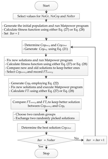
Figure 1.
The iterative algorithm of solving the optimal power flow (OPF) problem by using the modified coyote optimization algorithm (MCOA) method.
5. Simulation Results and Discussions
This section presents the simulation results from solving three transmission power systems with 30, 57, and 118 buses by using OCOA and the proposed MCOA. The whole data of the systems can be reached by referring to [11], meanwhile the coefficients of electric generation fuel cost function of IEEE 30-bus system are taken from [5]. In addition, the whole data are also supplemented together with the paper. For each considered objective, 50 successful runs were performed for obtaining 50 fitness functions corresponding to 50 optimal solutions. Then, main factors consisting of minimum, mean, and maximum of fitness function are reported for comparison. The implementation of the OCOA and the proposed MCOA was executed on the Matlab program language with version R2016a and personal computer with CPU: Intel Core i7-2.4GHz-RAM 4GB, GPU: Intel HD Graphics 5500, and operating system version: Windows 8.1 Pro-64-bit.
5.1. Result Comparisons between OCOA and MCOA for IEEE 30-Bus Transmission Power Network
5.1.1. Comparisons between OCOA and MCOA Methods for the Case without PVS
In this section, we compare the real performance of the proposed MCOA method with OCOA and other existing methods in finding optimal solutions for the IEEE 30-bus transmission power network with the two optimization cases consisting of power losses and fuel cost. For pair comparisons between the proposed method and OCOA, we set control parameters to the same values. However, the fair comparisons between the proposed method and other ones are based on the number of solution quality evaluations as well as the best fitness function values. Basically, the number of fitness evaluations for each trial run is also equivalent to the number of times that Matpower program had to be run. In the OPF problem, all dependent variables of each solution must be found and then both dependent variables and control variables are used to calculate the fitness function.
For the best observation of the performance comparisons between OCOA and MCOA, we executed OCOA and MCOA by setting different values to NoGr, NoCoy but fixing NoIter = 100. Table 1 and Table 2 report the results with three different settings for the cases of minimizing total fuel cost and total active power losses. Fitness function values of 50 successful runs are summarized by using minimum fitness, mean fitness, maximum fitness, and standard deviation. In addition to the results, the improvement of minimum fitness (IoMF) from the proposed method over OCOA and success rate (SR) in percent from the two methods are also calculated by using the following equations:

Table 1.
Results obtained by the original coyote optimization algorithm (OCOA) and MCOA for the EGFC objective of the IEEE 30-bus transmission power network with different settings of control parameters.
Table 2.
Result obtained by OCOA and MCOA for the total active power losses (TAPL) objective of the IEEE 30-bus transmission power network with different settings of control parameters.
Thus, improvement of minimum fitness and SR are also seen in the tables for a better view of performance comparison. The values of minimum fitness indicate that MCOA can find a much better optimal solution than OCOA for the different settings. For the cost objective, the best fitness of OCOA and MCOA are, respectively, $842.871 and $818.330 for the setting of NoGr = 3, NoCoy = 3, NoIter = 100, $829.244 and $799.899 for the setting of NoGr = 3, NoCoy = 4, NoIter = 100, and $801.643 and $798.916 for the setting of NoGr = 4, NoCoy = 4, NoIter = 100. Clearly, the proposed MCOA method can reach a better solution than OCOA for all the setting cases. The outstanding solutions can be evaluated by observing the improvement of minimum fitness that are 2.91%, 3.54%, and 0.34% corresponding to the three setting cases. Similarly, the proposed MCOA method also gets better mean fitness, maximum fitness, and standard deviation than OCOA for the three setting cases. Table 2 also indicates high performance of the proposed method over OCOA once the proposed method can reach much smaller values of total active power losses and the improvement of the minimum fitness is up to 29.45%, 30.21%, and 28.05% for three setting cases. Other values from the proposed method such as mean fitness, maximum fitness, and standard deviation are also less than those from OCOA. In the two tables, SR from MCOA is always higher than that from OCOA. In fact, MCOA can reach SR with 100% for the settings of NoGr = 3, NoCoy = 4, NoIter = 100 and NoGr = 4, NoCoy = 4, NoIter = 100 while the best SR from OCOA is 88% for the setting of NoGr = 4, NoCoy = 4, NoIter = 100. Therefore, MCOA outperforms OCOA in terms of constraint handling ability.
For a better view of outstanding performance of the proposed method over OCOA, 50 fitness function values of 50 successful runs and the convergence characteristic of the best run are plotted in Figure 2 and Figure 3 for the cost objective and in Figure 4 and Figure 5 for the loss objective. The figures are results from the setting of NoGr = 4, NoCoy = 4 and NoIter = 100. Figure 2 and Figure 4 show that the red curve has very tiny fluctuations and many red points have the same fitness as the best red point, while the blue curve has very high fluctuations and few blue points have smaller fitness than the worst red point. Figure 3 and Figure 5 point out the significantly faster search speed of the proposed method whereas OCOA is very slow. It can be seen that the fitness of the proposed method at the 20th iteration is much smaller than that of OCOA at the final iteration. Therefore, it can be stated that the proposed MCOA method is superior to OCOA in terms of:
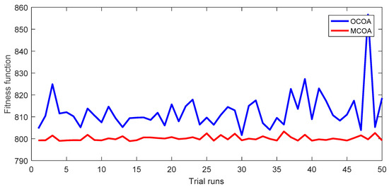
Figure 2.
The fitness function values of 50 successful runs obtained by OCOA and MCOA for the EGFC objective of the IEEE 30-bus transmission power network.
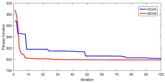
Figure 3.
Fitness function iteration characteristic of the best run from OCOA and MCOA for the EGFC objective of the IEEE 30-bus transmission power network.
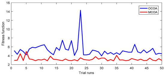
Figure 4.
The fitness function values of 50 successful runs obtained by OCOA and MCOA for the TAPL objective of the IEEE 30-bus transmission power network.
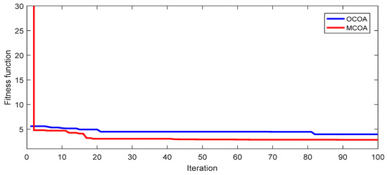
Figure 5.
Fitness function iteration characteristic of the best run from OCOA and MCOA for TAPL objective of the IEEE 30-bus transmission power network.
- 1
- Finding much better optimal solutions.
- 2
- Reaching more stable search ability.
- 3
- Converging to high quality solutions with significantly faster manner.
5.1.2. Comparisons between OCOA and MCOA Methods for the Case with PVS
In this section, we survey the real performance of OCOA and MCOA on a more complicated case of IEEE 30-bus system. A photovoltaic system with rated power of 2.0 MW was decided to be installed in the system. We suppose that geographical location of buses 3, 7, 8, 15, 18, 19, 20, 21, 22, 24, 26, 29, and 30 is appropriate for installing the PVS with power of 2.0 MW. We suppose the PVS uses an inverter to convert DC into AC without battery storage systems. Therefore, environment issue is not a problem in the installation of PV system. Thus, the duty of OCOA and MCOA in this studied case is to determine the location of installed PVS and other control variables of the conventional OPF problem. As a result, the control variable set for this studied case consists of SPi, Pk,i, Vk,i, Tt,i, and SVCc,i.
For implementing OCOA and MCOA for minimizing total power losses, we used the best setting of Section 5.1.1, i.e., NoGr = 4, NoCoy = 4, and NoIter = 100. The obtained results from the two methods over 50 successful runs including minimum, mean, and maximum power losses are compared. Results of total fuel cost are plotted in Figure 6, Figure 7 and Figure 8 meanwhile those of total power losses are plotted in Figure 9, Figure 10 and Figure 11. Figure 6 and Figure 7 indicate that OCOA and MCOA can reduce total fuel cost due to installing PVS. Namely, OCOA and MCOA can improve fuel cost by 0.7% and 0.88%. Similarly, Figure 9 and Figure 10 also show less power losses from OCOA and MCOA with PVS. Namely, OCOA and MCOA can improve power loss by 8.5% and 3.8%. As comparing results from OCOA and MCOA for the case of installing PVS, Figure 8 and Figure 11 show better cost and better loss of MCOA, respectively. As compared to OCOA, MCOA can improve fuel cost up to 0.51% and power loss up to 24.36%. Clearly, installing PVS can support OCOA and MCOA find better solutions with less total cost and less power losses.
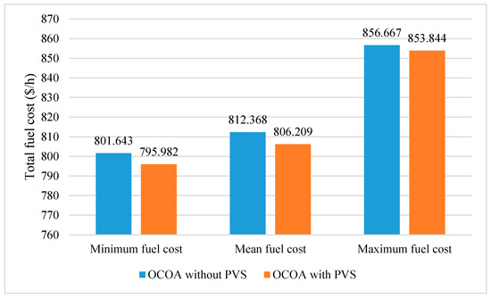
Figure 6.
Comparison of total fuel cost obtained by OCOA for the cases with and without PVS.
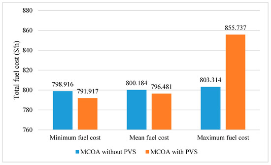
Figure 7.
Comparison of total fuel cost obtained by MCOA for the cases with and without PVS.
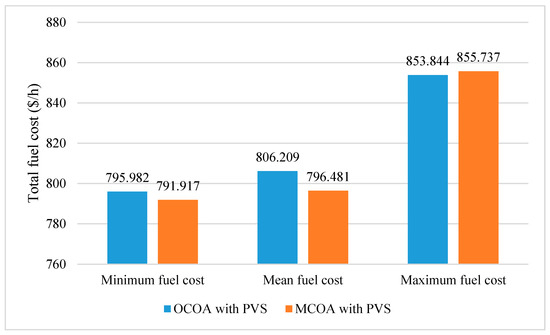
Figure 8.
Comparison of total fuel cost obtained by OCOA and MCOA for the case with PVS.
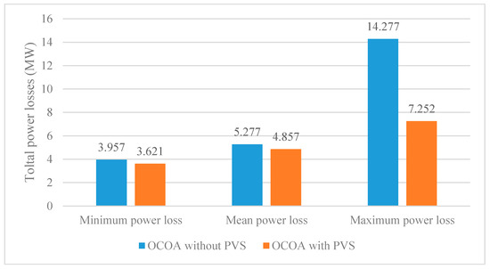
Figure 9.
Comparison of total power losses obtained by OCOA for the cases with and without PVS.
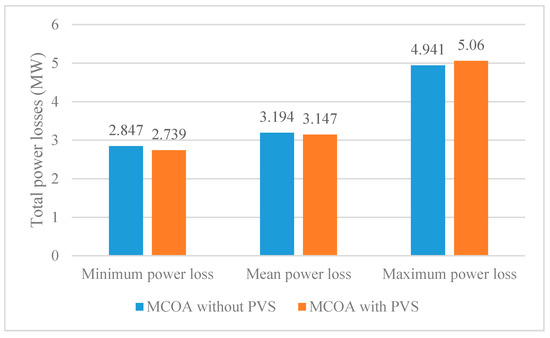
Figure 10.
Comparison of total power losses obtained by MCOA for the cases with and without PVS.
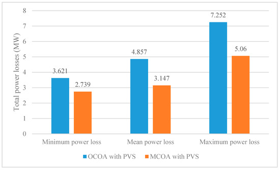
Figure 11.
Comparison of total power losses obtained by OCOA and MCOA for the case with PVS.
The best location of PVS found by OCOA and MCOA is, respectively, at buses 30 and 15 for fuel cost objective, and at buses 22 and 30 for power loss objective. Figure 12 and Figure 13 show the IEEE 30-bus system with the installation of PVS found by MCOA.
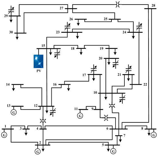
Figure 12.
The best location of PVS found by MCOA for the case of reducing total fuel cost.
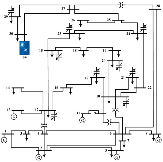
Figure 13.
The best location of PVS found by MCOA for the case of reducing total power losses.
5.2. Comparisons of Result from MCOA and Other Method for the IEEE 30-Bus Power System
Comparisons of total fuel cost and total power losses from MCOA and other methods are shown in Table 3 and Table 4, respectively. In addition to the best, mean, and worst values of cost and loss, three other factors including population size, the maximum number of iterations, and the number of solution quality evaluations are also mentioned for performance comparisons. Among the factors, population size and the number of solution quality evaluations of the proposed method are calculated by using the following equations:
Table 3.
Comparison of EGFC obtained by MCOA and other methods for the IEEE 30-bus transmission power network.
Table 4.
Comparison of TAPL obtained by MCOA and other methods for the IEEE 30-bus transmission power network.
Although the population size of other methods is a known factor, the number of solution quality evaluations must be calculated [38]. The best cost reported in Table 3 and the best power loss reported in Table 4 can reveal that the proposed method is more effective than other compared methods in finding higher quality solutions since its best cost and loss are less than those of others. In fact, the proposed method can reduce the cost from $0.0776 to $3.342 and the loss from 0.006 to 2.22 MW corresponding to the improvement level from 0.01% to 0.417% for the cost and from 0.21% to 43.88% for the loss. The mean and the maximum cost indicate that the proposed method and other ones have approximately equal stabilization because the deviation is not high. The mean and the maximum power loss of other methods have not been reported for comparison. In addition, the number of solution quality evaluations between the proposed and other ones should be mentioned. NoSqe of the proposed method is 2000 while that of others is much higher, from 4500 to 25,000 excluding SSO and ISSO with NoSqe = 690. However, the best cost and the best loss from SSO and ISSO are higher than those of the proposed method. Consequently, it can be concluded that the proposed method is more effective than other ones for the IEEE 30-bus transmission power network.
5.3. Result Comparisons for the IEEE 57-Bus Transmission Power Network
In the section, the proposed method is compared to OCOA and other methods based on results from minimizing fuel cost and power losses of the IEEE 57-bus transmission power system. OCOA and MCOA are executed by setting NoGr = 4, NoCoy = 4, and NoIter = 250. Comparisons of cost and loss for the system are shown in Table 5 and Table 6, while fitness function values of 50 runs and the best convergence characteristic of OCOA and MCOA are shown in Figure 14, Figure 15, Figure 16 and Figure 17. Comparisons between OCOA and MCOA show that MCOA can find less cost and less power loss than OCOA by $360.38 and 2.03 MW. These better results are corresponding to the improvement level of 0.86% and 17.3%. In addition, the mean and the maximum cost and loss of MCOA are also less than those of OCOA. For the network, MCOA and OCOA can reach SR with 96% and 74%, respectively. Therefore, MCOA still gets better ability of handling constraints than OCOA. With respect to graphic comparisons shown in Figure 14, Figure 15, Figure 16 and Figure 17 for 50 successful runs and the best convergence characteristic, MCOA also shows smaller fluctuations, high number of better solutions, and faster convergence speed. Therefore, the proposed MCOA method is really more robust than OCOA in finding the best solutions, reaching higher success rate, having better stabilization of the search process, and converging to a solution faster.
Table 5.
Comparison of EGFC obtained by MCOA and other methods for the IEEE 57-bus transmission power network.
Table 6.
Comparison of TAPL obtained by MCOA and other methods for the IEEE 57-bus transmission power network.
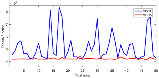
Figure 14.
The fitness function values of 50 successful runs obtained by OCOA and MCOA for the EGFC objective of the IEEE 57-bus transmission power network.
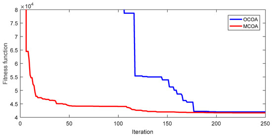
Figure 15.
Fitness function iteration characteristic of the best run from OCOA and MCOA for the EGFC objective of the IEEE 57-bus transmission power network.
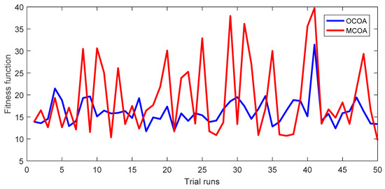
Figure 16.
The fitness function values of 50 successful runs obtained by OCOA and MCOA for the TAPL objective of the IEEE 57-bus transmission power network.
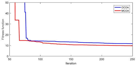
Figure 17.
Fitness function iteration characteristic of the best run from OCOA and MCOA for the TAPL objective of the IEEE 57-bus transmission power network.
The comparisons between the proposed MCOA and other ones emphasize that the proposed method is more effective than other ones since it can find less cost and less loss than all methods. As compared to the second best method and the worst method, the proposed MCOA can find less cost by $6.63 and $450.81, and less power loss by 2.81 MW and 2.77 MW. The results were converted to improvement level and this is 0.02% and 1.07% for cost, and 2.82% and 22.2% for power loss. Furthermore, the proposed method is also faster than nearly all methods because NoSqe of the proposed method is 5000 while that of other is from 5000 to 110,000 excluding SSO and ISSO with NoSqe = 1700. Therefore, it can be concluded that the proposed method is really effective for the IEEE 57-bus transmission power network.
5.4. Result Comparisons for the IEEE 118-Bus Transmission Power Network
In the section, the IEEE 118-bus transmission power network is employed as the most complicated study case with 118 buses and 130 control variables. NoGr, NoCoy and NoIter were, respectively, set to 5, 5, and 300. From these settings, Npop and NoSqe from OCOA and MCOA are calculated to be 25 and 9000. Result comparisons are shown in Table 7. For the test system, both MCOA and OCOA cannot reach SR of 100% due to the impact of the large scale system. However, the success rate of the proposed MCOA is much higher than that of OCOA since SR of OCOA and MCOA is, respectively, 16% and 52%. SR from other compared methods in Table 7 was not reported in previous studies, so we cannot compare the constraint handling ability of the proposed method and these ones. For comparison of the best cost, the proposed method can find less cost than OCOA by $2469.78 corresponding to the improvement of 1.87%. As observing minimum cost of all methods, the proposed method can reach a better optimal solution than all methods with less cost by $168.91 to $9098.85, corresponding to the improvement from 0.13% to 6.55%. The reported values are not compared to GPUA-PSO because study [12] did not report control variables for checking. The mean cost and the worst cost of the proposed method are less than those of all methods. Furthermore, NoSqe of the proposed method is 9000 while that of others is from 9000 to 225,000. Therefore, the proposed method is superior to all compared methods and it is really powerful for the IEEE 118-bus transmission power network.
Table 7.
Comparison of EGFC obtained by MCOA and other methods for the IEEE 118-bus transmission power network.
In the Appendix A, optimal control variables reached by the proposed MCOA are presented in Table A1, Table A2, Table A3 and Table A4.
5.5. Discussion
OCOA and MCOA are meta-heuristic algorithms based on randomizations similarly to other meta-heuristic algorithms such as GA, PSO, DE, etc. In the structure of search process, OCOA is particularly dependent on randomizations, especially the second generation in Equation (17) with three variable selection choices, varn,pr1,g, varn,pr2,g, and varn,rd. Furthermore, the selection of one out of the three variables is decided by another randomization condition. That is either or . In addition, in the step of exchanging solutions, OCOA is also based on one more randomization condition of . The randomizations are not effective, but they are time consuming. Therefore, we modified Equation (17) and canceled using the condition for exchanging solutions. The task can reduce ineffective computation steps as well as shorten execution time. As a result, MCOA can avoid the ineffective randomizations. However, MCOA cannot eliminate randomizations completely as shown in Equation (21) and (22) and the task of exchanging solutions. The randomization in Equations (21) and (22) are the characteristic of meta-heuristic algorithms because the randomizations can support production of different solutions similarly to PSO, DE, etc. The randomization in exchanging solutions is also useful for avoiding lumping all solutions in each group, leading to a very low possibility of converging local optimum. Consequently, MCOA solved the OPF problem more effectively than OCOA. In Section 5.1.1 and Section 5.1.2, we ran OCOA and MCOA by setting different values to the number of groups and the number of coyotes in each group. The result comparisons indicated that MCOA was completely more effective than OCOA. For each study case, we ran the two methods, and 50 trials and results in terms of minimum, mean, and maximum fitness are reported in Table 1 and Table 2 and Figure 6, Figure 7, Figure 8, Figure 9, Figure 10 and Figure 11. The result comparisons indicate that MCOA can reach better solutions than OCOA with less fuel cost and less power losses.
For solving the three systems, the proposed MCOA tackled several disadvantages that its original method suffered such as slowly finding high quality solutions, having a high impact on randomizations, owning a high number of computation steps, and using a long simulation time. As shown in sections above, the proposed method could reach better results than OCOA such as
- 1
- Finding higher quality solutions: the best fuel cost and the best total power loss of MCOA are less than those from OCOA for all study cases,
- 2
- Having more stable search ability: figures showing fitness function of 50 trial runs indicated that approximately all runs of MCOA had lower fitness function than those of OCOA,
- 3
- Reducing simulation time: MCOA can reduce a number of computation steps by canceling randomizations in the first and the second generations. Furthermore, the fast search speed can reduce the number of iterations and shorten simulation time.
However, we had to cope with several difficulties to reach high performance for the search process of the proposed MCOA in dealing with the OPF problem, especially for a large scale system with 118 buses and a high number of control variable cases such as the case with installation of PVS for the IEEE 30-bus system. As we knew, the proposed MCOA method has three basic control parameters including the number of coyotes in each group NoCoy, the number of groups NoGr, and the number of iterations NoIter. The population size of the proposed MCOA method is equal to (NoGr × NoCoy) meanwhile the number of new solutions produced for each iteration and for one run is, respectively, (NoGr × NoCoy + NoGr) and (NoGr × NoCoy + NoGr) × NoIter. Therefore, the task of tuning the most appropriate values for NoCoy, NoGr, and NoIter is not easy. In fact, during the implementation of the proposed MCOA we considered the comparison criterion, which is the number of solution quality evaluations NoSqe shown in Equation (40). As shown in Table 1 and Table 2, we set different values for NoCoy and NoGr but fixed NoIter = 100. However, it is just one setting of the trial settings for reaching the best results of MCOA. During the implementation, we also reduced NoIter and increased the result of (NoGr × NoCoy). For the setting of (NoGr × NoCoy), we also increased NoGr or NoCoy and decreased the remaining one. As a result, we concluded the most appropriate setting for the parameters and we applied the settings for all study cases of the considered system. Results shown in sections above indicated that four was the best value for both NoGr and NoCoy for the IEEE 30-bus system and IEEE 57-bus system but five was the best value for both NoGr and NoCoy for the IEEE 118-bus system. It is clear that the setting of the control parameters of MCOA is not an easy task and it must take long simulation time. The difficulty will become more serious if the selection of control variables is not certain and there are many choices of control variables. Fortunately, the OPF problem is complicated but the selection of control variables is predetermined by using the MatPower program. As using the Matpower program, input data must be active power output of all generators excluding generator at slack bus, voltage of all generators, reactive power output of capacitors, and tap changer of transformers. Therefore, all the variables are predetermined as control variables and there is no difficulty for the selection of control variables. For the case of installing PVS, the position of one load bus must be selected for providing 2.0 MW to the load and reducing 2.0 MW supplied from the transmission lines. Therefore, the selection of control variables was also an easy task for the more complicated case of installing PVS. In the future, we will consider other clean power sources such as wind turbines and hydropower plants as a real power system. In addition, a multi-period problem will be studied instead of single period problem in this study. In daytime hours, PVS together with other sources will supply electricity to the load but the presence of PVS will not be taken into account at night. The task of the new problem is to determine the best location for installing PVS and wind turbines meanwhile the location of hydropower plants and thermal power plants is known.
6. Conclusions
In this paper, a novel coyote optimization algorithm was proposed for solving the OPF problem. The proposed method was developed by modifying two techniques of generating new solutions and one technique of exchanging solutions among available groups. By testing on IEEE 30, 57, and 118-bus transmission power networks with two cases of minimizing electric generation fuel cost and total active power losses, the proposed method was demonstrated to be more effective and robust than OCOA in terms of better quality of the best solution, better stabilization of search process, faster convergence, and higher success rate. The result comparisons are as follows:
- 1
- The best success rate of the proposed method the three systems was, respectively, 100%, 96%, and 52%, meanwhile that of OCOA was, respectively, 88%, 74%, and 16%.
- 2
- The improvement level of cost from MCOA over OCOA could be up to 3.54% while the improvement level for power loss could be up to 30.21%.
As compared to other methods, the method could be more effective in finding better solutions with a faster manner. The result comparisons can be summarized as follows:
- The proposed method could obtain improvement levels of cost and loss as 0.417% and 43.88% for the IEEE 30-bus transmission power network, and 1.07% and 22.2% for the IEEE 57-bus transmission power network, while the improvement level of cost for IEEE 118-bus transmission power network was 6.55%.
- The proposed method used either an equal or smaller number of solution quality evaluations.
For further investigation of the performance, OCOA and MCOA were run to install a PVS in the IEEE 30-bus system. The results were promising as follows:
- 1
- Both OCOA and MCOA could reduce the cost by 0.7%–8.5% and the power loss by 8.5% and 3.8%.
- 2
- As compared to OCOA, MCOA could reduce fuel cost and power loss by 0.5% and 24.36%, respectively.
Consequently, it is recommended that MCOA is a favorable optimization tool for solving the OPF problem and for more complicated studies with the presence of renewable energies.
Author Contributions
Z.L. and Y.C. simulated results and wrote important parts of the article. L.V.D. and X.Y. selected references, formatted the whole paper, summarized results in Tables, and wrote the introduction. T.T.N. edited the whole paper.
Funding
This research was funded by the National Natural Science Foundation of China (NSFC) under project No. 51520105011.
Conflicts of Interest
The authors declare that there is no conflict of interests regarding the publication of this paper.
Abbreviations
| ABCA | Artificial bee colony algorithm |
| ACO | Ant colony optimization |
| AGSO | Adaptive group search optimization |
| BA | Bat Algorithm |
| BSA | Backtracking Search algorithm |
| COA | Cuckoo optimization algorithm |
| DSM | Differential search method |
| EACO | Enhanced ant colony optimization |
| FA | Firefly algorithm |
| GBBICM | Gaussian bare-bones imperialist competitive method |
| GSA | Gravitational search algorithm |
| GWOA | Grey Wolf Optimization algorithm |
| IBA | Improved bat algorithm |
| IEEE | Institute of Electrical and Electronics Engineers |
| IHBMO | Improved honey bee mating optimization |
| IICM | Improved imperialist competitive method |
| ISSO | Improved social spider optimization |
| ITLBO | Improved teaching learning based optimization |
| MCBOM | Modified Colliding Bodies Optimization method |
| MELMM | Modified electromagnetism-like Mechanism method |
| MFO | Moth-flame Optimizer |
| MPM | Mathematical programming method |
| MSCA | Modified Sine-Cosine algorithm |
| MSM | Moth swarm method |
| SaDE | Self-adaptive Differential Evolution |
| SCA | Sine-Cosine algorithm |
| SKHM | Stud krill herd method |
| SOSA | Symbiotic Organism Search algorithm |
| SSO | Social spider optimization |
| TSA | Tree-seed algorithm |
| Nomenclature | |
| Susceptance and conductance of the feeder connecting bus j and bus i | |
| C1, C2, C3, C4 | Penalty factors |
| Coycen,g | The center solution of the gth group |
| Coym,g | The mth solution in the gth group |
| Coypr1,g, Coypr2,g | Two randomly picked solutions from the gth group |
| Coyworst,g | The worst solution in the gth group |
| CoyGbest | The best solution in the whole population |
| CVari | The control variable set of the ith solution |
| ∆MVAbr,i | The penalty term for the violation of apparent power of the brth feeder corresponding to the ith solution |
| ∆P1,i | The penalty term for the violation of active power at slack bus corresponding to the ith solution |
| ∆Qk,i | The penalty term for the violation of reactive power at the kth generator bus corresponding to the ith solution |
| ∆VLl,i | The penalty term for the violation of voltage at the lth load bus corresponding to the ith solution |
| EGFC | The total electric generation fuel cost of all thermal power plants |
| EGFCk,i | The electric generation fuel cost of the kth thermal power plant corresponding to the ith solution |
| FTi | Fitness function of the ith solution |
| Phase angles of voltage at the jth bus and the ith bus | |
| FTworst,g | Fitness value of the worst solution in the gth group |
| Iter | Current iteration |
| λ1, λ2, λ3, λ4, λ5, λ6, λ7, λ8, λ9, λ10, λ11 | Randomly generated numbers in the range from 0 to 1 |
| The apparent power flowing through the brth transmission of the ith solution | |
| The highest apparent power of the brth feeder | |
| NoB | The number of buses in the considered transmission power network |
| NoBR | The number of transmission branches in the considered transmission grid |
| NoCV | The number of control variables included in each solution |
| NoCoy | The number of solutions in each group |
| NoGr | The number of groups |
| NoIter | The maximum number of iterations |
| NoL | The number of load buses in the considered transmission grid |
| NoSqe | The number of solution quality evaluations |
| NoS | The number of solutions or population size |
| NoSVC | The number of static VAR compensators in the considered transmission grid |
| NoT | The number of transformers |
| Npop | Population size |
| P1,i | Active power of the thermal power plant at slack bus corresponding to the ith solution |
| Pj, Qj | Active and reactive power generated at the jth bus |
| Pk,i, Qk,i, Vk,i | Active power, reactive power and voltage of the kth thermal power plant corresponding to the ith solution |
| The smallest and highest active power output of the kth thermal power plant | |
| The smallest and highest active power output of the thermal power plant at slack bus | |
| PLj | Active power demand of the load at the jth bus |
| PLk | The active power demand at the kth bus |
| The smallest and highest reactive power output of the kth thermal power plant | |
| SP | Site of photovoltaic system |
| SPi | Site of photovoltaic system corresponding to the ith solution |
| SVCc,i | The reactive power of the cth static VAR compensator corresponding to the ith solution |
| SVCj | The reactive power of static VAR compensator generated at the jth bus |
| Lower bound and upper bound of the cth static VAR compensator | |
| Tt,i | Tap changer of the tth transformer corresponding to the ith solution |
| Tmin, Tmax | The smallest tap changer and the highest tap changer of transformers |
| Lower bound and upper bound of voltage of thermal power plant generators | |
| Vi, Vj | Magnitude of voltage at the ith bus and the jth bus |
| Varn,g | The nth control variable of the solution in the gth group |
| VLl,i | Voltage of load at the lth load bus corresponding to the ith solution |
| VLmin, VLmax | Lower bound and upper bound of load bus voltage |
Appendix A
Table A1.
Control variables obtained by the proposed MCOA method for the IEEE 30-bus transmission power network.
Table A1.
Control variables obtained by the proposed MCOA method for the IEEE 30-bus transmission power network.
| Variable | EGFC Objective | TAPL Objective |
|---|---|---|
| PG1 | 177.2642 | 51.2489 |
| PG2 | 48.7616 | 80.0000 |
| PG5 | 21.1802 | 50.0000 |
| PG8 | 20.6942 | 35.0000 |
| PG11 | 12.0994 | 30.0000 |
| PG13 | 12.0066 | 39.9980 |
| VG1 | 1.1000 | 1.1000 |
| VG2 | 1.0879 | 1.1000 |
| VG5 | 1.0608 | 1.0820 |
| VG8 | 1.0682 | 1.0899 |
| VG11 | 1.0999 | 1.1000 |
| VG13 | 1.1000 | 1.1000 |
| Qc1 | 5.0000 | 4.3753 |
| Qc2 | 4.7782 | 0.0001 |
| Qc3 | 4.3765 | 4.9727 |
| Qc4 | 4.5808 | 5.0000 |
| Qc5 | 4.8757 | 5.0000 |
| Qc6 | 5.0000 | 5.0000 |
| Qc7 | 3.3788 | 1.0161 |
| Qc8 | 4.9352 | 5.0000 |
| Qc9 | 2.7671 | 1.2002 |
| T11 | 1.0389 | 1.0598 |
| T12 | 0.9000 | 0.9066 |
| T15 | 0.9827 | 0.9758 |
| T36 | 0.9658 | 0.9667 |
Table A2.
Optimal solutions obtained by MCOA for the case with PVS in the IEEE 30-bus system.
Table A2.
Optimal solutions obtained by MCOA for the case with PVS in the IEEE 30-bus system.
| Variable | Optimize Total Power Losses | Optimize Total Fuel Cost |
|---|---|---|
| PG1 | 50.1323 | 177.3232 |
| PG2 | 79.0242 | 47.7038 |
| PG5 | 50 | 21.0492 |
| PG8 | 34.9821 | 21.3667 |
| PG11 | 30 | 10.5512 |
| PG13 | 40 | 12.0120 |
| VG1 | 1.1 | 1.1000 |
| VG2 | 1.096 | 1.0862 |
| VG5 | 1.0806 | 1.0533 |
| VG8 | 1.0888 | 1.0649 |
| VG11 | 1.1 | 1.1000 |
| VG13 | 1.1 | 1.0984 |
| Qc1 | 0 | 4.9479 |
| Qc2 | 4.7165 | 4.8779 |
| Qc3 | 5 | 4.8243 |
| Qc4 | 5 | 3.9381 |
| Qc5 | 5 | 2.6789 |
| Qc6 | 4.2267 | 4.6555 |
| Qc7 | 1.2101 | 3.0685 |
| Qc8 | 4.9853 | 3.9158 |
| Qc9 | 3.5789 | 4.9469 |
| T11 | 0.9434 | 0.9508 |
| T12 | 1.1 | 0.9977 |
| T15 | 1.0115 | 0.9883 |
| T36 | 1.0037 | 0.9762 |
| SP | 30 | 15 |
Table A3.
Control variables obtained by the proposed MCOA method for the IEEE 57-bus transmission power network.
Table A3.
Control variables obtained by the proposed MCOA method for the IEEE 57-bus transmission power network.
| Variable | Fuel Cost Minimization | Power Loss Minimization |
|---|---|---|
| PG1 | 144.9455 | 209.1483 |
| PG2 | 89.9556 | 3.0094 |
| PG3 | 44.8814 | 140 |
| PG6 | 64.8987 | 100 |
| PG8 | 460.005 | 299.3124 |
| PG9 | 99.3167 | 99.2739 |
| PG12 | 361.3249 | 409.7594 |
| VG1 | 1.0981 | 1.1 |
| VG2 | 1.091 | 1.0944 |
| VG3 | 1.0907 | 1.0999 |
| VG6 | 1.1 | 1.0985 |
| VG8 | 1.1 | 1.0969 |
| VG9 | 1.0805 | 1.0793 |
| VG12 | 1.0938 | 1.0893 |
| Qc1 | 9.8097 | 0 |
| Qc2 | 5.1456 | 5.0375 |
| Qc3 | 6.2944 | 6.3 |
| T1 | 1.1 | 1.1 |
| T2 | 1.0981 | 0.9 |
| T3 | 1.0701 | 1.005 |
| T4 | 1.0309 | 0.9001 |
| T5 | 0.9416 | 0.95 |
| T6 | 1.0057 | 0.9642 |
| T7 | 0.9885 | 0.9866 |
| T8 | 0.9467 | 0.9005 |
| T9 | 0.9 | 0.9002 |
| T10 | 0.987 | 0.9899 |
| T11 | 0.953 | 0.9945 |
| T12 | 0.9808 | 1.0009 |
| T13 | 0.9518 | 0.9524 |
| T14 | 0.9906 | 1.0826 |
| T15 | 1.0194 | 1.0722 |
| T16 | 0.9794 | 0.9279 |
| T17 | 1.0053 | 0.9868 |
Table A4.
Control variables obtained by the proposed MCOA method for the IEEE 118-bus transmission power network.
Table A4.
Control variables obtained by the proposed MCOA method for the IEEE 118-bus transmission power network.
| Control Variable | Value | Control Variable | Value | Control Variable | Value |
|---|---|---|---|---|---|
| P1 (MW) | 24.8557 | P103 (MW) | 38.0638 | V76 (PU) | 1.004 |
| P4 (MW) | 0.023 | P104 (MW) | 0.4972 | V77 (PU) | 1.0311 |
| P6 (MW) | 0.0015 | P105 (MW) | 1.5594 | V80 (PU) | 1.0435 |
| P8 (MW) | 0.0767 | P107 (MW) | 34.5069 | V85 (PU) | 1.028 |
| P10 (MW) | 399.7336 | P110 (MW) | 11.6535 | V87 (PU) | 1.0372 |
| P12 (MW) | 86.179 | P111 (MW) | 36.2049 | V89 (PU) | 1.0447 |
| P15 (MW) | 20.4286 | P112 (MW) | 33.962 | V90 (PU) | 1.0211 |
| P18 (MW) | 11.7113 | P113 (MW) | 0.3254 | V91 (PU) | 1.0209 |
| P19 (MW) | 22.2119 | P116 (MW) | 0.0002 | V92 (PU) | 1.0304 |
| P24 (MW) | 0.236 | V1 (PU) | 1.0005 | V99 (PU) | 1.0332 |
| P25 (MW) | 194.5895 | V4 (PU) | 1.0296 | V100 (PU) | 1.0379 |
| P26 (MW) | 281.4839 | V6 (PU) | 1.0211 | V103 (PU) | 1.0335 |
| P27 (MW) | 11.4272 | V8 (PU) | 1.0781 | V104 (PU) | 1.0188 |
| P31 (MW) | 7.3547 | V10 (PU) | 1.0929 | V105 (PU) | 1.0169 |
| P32 (MW) | 14.089 | V12 (PU) | 1.0157 | V107 (PU) | 1.0118 |
| P34 (MW) | 3.3261 | V15 (PU) | 1.0162 | V110 (PU) | 1.0527 |
| P36 (MW) | 4.4716 | V18 (PU) | 1.0202 | V111 (PU) | 1.0867 |
| P40 (MW) | 46.8342 | V19 (PU) | 1.0167 | V112 (PU) | 1.0474 |
| P42 (MW) | 38.953 | V24 (PU) | 1.0394 | V113 (PU) | 1.0263 |
| P46 (MW) | 19.2667 | V25 (PU) | 1.0587 | V116 (PU) | 1.0505 |
| P49 (MW) | 193.4075 | V26 (PU) | 1.0871 | SVC5 (MVAr) | −0.1794 |
| P54 (MW) | 49.3797 | V27 (PU) | 1.0211 | SVC34 (MVAr) | 0.0217 |
| P55 (MW) | 32.1311 | V31 (PU) | 1.0125 | SVC37 (MVAr) | −0.0246 |
| P56 (MW) | 37.4034 | V32 (PU) | 1.0187 | SVC44 (MVAr) | 0.0024 |
| P59 (MW) | 149.0935 | V34 (PU) | 1.0257 | SVC45 (MVAr) | 0.0011 |
| P61 (MW) | 147.9593 | V36 (PU) | 1.0232 | SVC46 (MVAr) | 0.0146 |
| P62 (MW) | 0.009 | V40 (PU) | 1.0122 | SVC48 (MVAr) | 0.0047 |
| P65 (MW) | 352.0099 | V42 (PU) | 1.0119 | SVC74 (MVAr) | 0.0026 |
| P66 (MW) | 349.0427 | V46 (PU) | 1.032 | SVC79 (MVAr) | 0.0593 |
| P70 (MW) | 0.1006 | V49 (PU) | 1.043 | SVC82 (MVAr) | 0.0059 |
| P72 (MW) | 0.0192 | V54 (PU) | 1.0165 | SVC83 (MVAr) | 0.1876 |
| P73 (MW) | 0.7076 | V55 (PU) | 1.0151 | SVC105 (MVAr) | 0.0983 |
| P74 (MW) | 14.0153 | V56 (PU) | 1.0152 | SVC107 (MVAr) | 0 |
| P76 (MW) | 35.1036 | V59 (PU) | 1.0329 | SVC110 (MVAr) | 0.0069 |
| P77 (MW) | 0.0044 | V61 (PU) | 1.0362 | T8 (pu) | 1.0361 |
| P80 (MW) | 428.8456 | V62 (PU) | 1.0363 | T32 (pu) | 1.0135 |
| P85 (MW) | 0.0897 | V65 (PU) | 1.0626 | T36 (pu) | 1.0298 |
| P87 (MW) | 3.6106 | V66 (PU) | 1.0535 | T51 (pu) | 1.0152 |
| P89 (MW) | 498.136 | V69 (PU) | 1.066 | T93 (pu) | 0.9999 |
| P90 (MW) | 0.0061 | V70 (PU) | 1.0398 | T95 (pu) | 1.0153 |
| P91 (MW) | 0.0414 | V72 (PU) | 1.0396 | T102 (pu) | 0.9929 |
| P92 (MW) | 0.0123 | V73 (PU) | 1.0446 | T107 (pu) | 0.9344 |
| P99 (MW) | 0.3744 | V74 (PU) | 1.0135 | T127 (pu) | 0.9971 |
| P100 (MW) | 229.5969 | - | - | - | - |
References
- Nguyen, T.T.; Quynh, N.V.; Van Dai, L. Improved Firefly Algorithm: A Novel Method for Optimal Operation of Thermal Generating Units. Complexity 2018, 2018. [Google Scholar] [CrossRef]
- Nguyen, T.; Vo, D.; Vu Quynh, N.; Van Dai, L. Modified cuckoo search algorithm: A novel method to minimize the fuel cost. Energies 2018, 11, 1328. [Google Scholar] [CrossRef]
- Ongsakul, W.; Tantimaporn, T. Optimal power flow by improved evolutionary programming. Electr. Power Compon. Syst. 2006, 34, 79–95. [Google Scholar] [CrossRef]
- El-Fergany, A.A.; Hasanien, H.M. Single and multi-objective optimal power flow using grey wolf optimizer and differential evolution algorithms. Electr. Power Compon. Syst. 2015, 43, 1548–1559. [Google Scholar] [CrossRef]
- El Ela, A.A.; Abido, M.A.; Spea, S.R. Optimal power flow using differential evolution algorithm. Electr. Power Syst. Res. 2010, 80, 878–885. [Google Scholar] [CrossRef]
- Thitithamrongchai, C.; Eua-Arporn, B. Self-adaptive differential evolution based optimal power flow for units with non-smooth fuel cost functions. J. Electr. Syst. 2007, 3, 88–99. [Google Scholar]
- Sayah, S.; Zehar, K. Modified differential evolution algorithm for optimal power flow with non-smooth cost functions. Energy Convers. Manag. 2008, 49, 3036–3042. [Google Scholar] [CrossRef]
- Shaheen, A.M.; El-Sehiemy, R.A.; Farrag, S.M. Solving multi-objective optimal power flow problem via forced initialised differential evolution algorithm. IET Gener. Transm. Distrib. 2016, 10, 1634–1647. [Google Scholar] [CrossRef]
- Niknam, T.; Narimani, M.R.; Aghaei, J.; Azizipanah-Abarghooee, R. Improved particle swarm optimisation for multi-objective optimal power flow considering the cost, loss, emission and voltage stability index. IET Gener. Transm. Distrib. 2012, 6, 515–527. [Google Scholar] [CrossRef]
- Vaisakh, K.; Srinivas, L.R.; Meah, K. Genetic evolving ant direction particle swarm optimization algorithm for optimal power flow with non-smooth cost functions and statistical analysis. Appl. Soft Comput. 2013, 13, 4579–4593. [Google Scholar] [CrossRef]
- Vo, D.N.; Schegner, P. An Improved Particle Swarm Optimization for Optimal Power Flow. In Meta-Heuristics Optimization Algorithms in Engineering, Business, Economics, and Finance; IGI Global: Hershey, PA, USA, 2013; pp. 1–40. [Google Scholar]
- Roberge, V.; Tarbouchi, M.; Okou, F. Optimal power flow based on parallel metaheuristics for graphics processing units. Electr. Power Syst. Res. 2016, 140, 344–353. [Google Scholar] [CrossRef]
- Marcelino, C.G.; Almeida, P.E.; Wanner, E.F.; Baumann, M.; Weil, M.; Carvalho, L.M.; Miranda, V. Solving security constrained optimal power flow problems: A hybrid evolutionary approach. Appl. Intell. 2018, 48, 3672–3690. [Google Scholar] [CrossRef]
- Saini, A.; Chaturvedi, D.K.; Saxena, A.K. Optimal power flow solution: a GA-fuzzy system approach. Int. J. Emerg. Electr. Power Syst. 2006, 5. [Google Scholar] [CrossRef]
- Kumari, M.S.; Maheswarapu, S. Enhanced genetic algorithm based computation technique for multi-objective optimal power flow solution. Int. J. Electr. Power Energy Syst. 2010, 32, 736–742. [Google Scholar] [CrossRef]
- Reddy, S.S.; Bijwe, P.R.; Abhyankar, A.R. Faster evolutionary algorithm based optimal power flow using incremental variables. Int. J. Electr. Power Energy Syst. 2014, 54, 198–210. [Google Scholar] [CrossRef]
- Reddy, S.S.; Bijwe, P.R. Efficiency improvements in meta-heuristic algorithms to solve the optimal power flow problem. Int. J. Electr. Power Energy Syst. 2016, 82, 288–302. [Google Scholar] [CrossRef]
- Shabanpour-Haghighi, A.; Seifi, A.R.; Niknam, T. A modified teaching–learning based optimization for multi-objective optimal power flow problem. Energy Convers. Manag. 2014, 77, 597–607. [Google Scholar] [CrossRef]
- Daryani, N.; Hagh, M.T.; Teimourzadeh, S. Adaptive group search optimization algorithm for multi-objective optimal power flow problem. Appl. Soft Comput. 2016, 38, 1012–1024. [Google Scholar] [CrossRef]
- Niknam, T.; Narimani, M.R.; Aghaei, J.; Tabatabaei, S.; Nayeripour, M. Modified honey bee mating optimisation to solve dynamic optimal power flow considering generator constraints. IET Gener. Transm. Distrib. 2011, 5, 989–1002. [Google Scholar] [CrossRef]
- Ara, A.L.; Kazemi, A.; Gahramani, S.; Behshad, M. Optimal reactive power flow using multi-objective mathematical programming. Sci. Iran. 2012, 19, 1829–1836. [Google Scholar] [CrossRef]
- Duman, S.; Güvenç, U.; Sönmez, Y.; Yörükeren, N. Optimal power flow using gravitational search algorithm. Energy Convers. Manag. 2012, 59, 86–95. [Google Scholar] [CrossRef]
- Adaryani, M.R.; Karami, A. Artificial bee colony algorithm for solving multi-objective optimal power flow problem. Int. J. Electr. Power Energy Syst. 2013, 53, 219–230. [Google Scholar] [CrossRef]
- Ghasemi, M.; Ghavidel, S.; Ghanbarian, M.M.; Gharibzadeh, M.; Vahed, A.A. Multi-objective optimal power flow considering the cost, emission, voltage deviation and power losses using multi-objective modified imperialist competitive algorithm. Energy 2014, 78, 276–289. [Google Scholar] [CrossRef]
- Le Anh, T.N.; Vo, D.N.; Ongsakul, W.; Vasant, P.; Ganesan, T. Cuckoo optimization algorithm for optimal power flow. In Adaptation, Learning and Optimization, Proceedings of the 18th Asia Pacific Symposium on Intelligent and Evolutionary Systems; Springer: Berlin, Germany, 2015; Volume 1, pp. 479–493. [Google Scholar]
- Ladumor, D.P.; Trivedi, I.N.; Bhesdadiya, R.H.; Jangir, P. A grey wolf optimizer algorithm for Voltage Stability Enhancement. In Proceedings of the 2017 Third International Conference on Advances in Electrical, Electronics, Information, Communication and Bio-Informatics (AEEICB), Chennai, India, 27–28 February 2017. [Google Scholar]
- Ghasemi, M.; Ghavidel, S.; Ghanbarian, M.M.; Gitizadeh, M. Multi-objective optimal electric power planning in the power system using Gaussian bare-bones imperialist competitive algorithm. Inf. Sci. 2015, 294, 286–304. [Google Scholar] [CrossRef]
- El-Hana Bouchekara, H.R.; Abido, M.A.; Chaib, A.E. Optimal power flow using an improved electromagnetism-like mechanism method. Electr. Power Compon. Syst. 2016, 44, 434–449. [Google Scholar] [CrossRef]
- Bouchekara, H.R.E.H.; Chaib, A.E.; Abido, M.A.; El-Sehiemy, R.A. Optimal power flow using an Improved Colliding Bodies Optimization algorithm. Appl. Soft Comput. 2016, 42, 119–131. [Google Scholar] [CrossRef]
- Abaci, K.; Yamacli, V. Differential search algorithm for solving multi-objective optimal power flow problem. Int. J. Electr. Power Energy Syst. 2016, 1, 10–79. [Google Scholar] [CrossRef]
- Pulluri, H.; Naresh, R.; Sharma, V. A solution network based on stud krill herd algorithm for optimal power flow problems. Soft Comput. 2018, 22, 159–176. [Google Scholar] [CrossRef]
- Mohamed, A.A.A.; Mohamed, Y.S.; El-Gaafary, A.A.; Hemeida, A.M. Optimal power flow using moth swarm algorithm. Electr. Power Syst. Res. 2017, 142, 190–206. [Google Scholar] [CrossRef]
- Raviprabakaran, V.; Subramanian, R.C. Enhanced ant colony optimization to solve the optimal power flow with ecological emission. Int. J. Syst. Assur. Eng. Manag. 2018, 9, 58–65. [Google Scholar] [CrossRef]
- Trivedi, I.N.; Jangir, P.; Parmar, S.A.; Jangir, N. Optimal power flow with voltage stability improvement and loss reduction in power system using Moth-Flame Optimizer. Neural Comput. Appl. 2018, 30, 1889–1904. [Google Scholar] [CrossRef]
- Yuan, Y.; Wu, X.; Wang, P.; Yuan, X. Application of improved bat algorithm in optimal power flow problem. Appl. Intell. 2018, 48, 2304–2314. [Google Scholar] [CrossRef]
- El-Fergany, A.A.; Hasanien, H.M. Tree-seed algorithm for solving optimal power flow problem in large-scale power systems incorporating validations and comparisons. Appl. Soft Comput. 2018, 64, 307–316. [Google Scholar] [CrossRef]
- Attia, A.F.; Sehiemy, R.A.E.; Hasanien, H.M. Optimal power flow solution in power systems using a novel Sine-Cosine algorithm. Int. J. Electr. Power Energy Syst. 2018, 99, 331–343. [Google Scholar] [CrossRef]
- Nguyen, T.T. A high performance social spider optimization algorithm for optimal power flow solution with single objective optimization. Energy 2019, 171, 218–240. [Google Scholar] [CrossRef]
- Pierezan, J.; Coelho, L.D.S. Coyote Optimization Algorithm: A New Metaheuristic for Global Optimization Problems. IEEE Congr. Evol. Comput. 2018, 1–8. [Google Scholar] [CrossRef]
- Qais, M.H.; Hasanien, H.M.; Alghuwainem, S.; Nouh, A.S. Coyote optimization algorithm for parameters extraction of three-diode photovoltaic models of photovoltaic modules. Energy 2019, 187, 116001. [Google Scholar] [CrossRef]
- Pierezan, J.; Maidl, G.; Yamao, E.M.; dos Santos Coelho, L.; Mariani, V.C. Cultural coyote optimization algorithm applied to a heavy duty gas turbine operation. Energy Convers. Manag. 2019, 199, 111932. [Google Scholar] [CrossRef]
- Güvenç, U.; Kaymaz, E. Economic Dispatch Integrated Wind Power Using Coyote Optimization Algorithm. In Proceedings of the 2019 7th International Istanbul Smart Grids and Cities Congress and Fair (ICSG), Istanbul, Turkey, 25–26 April 2019; pp. 179–183. [Google Scholar]
- Nguyen, T.T.; Vo, D.N. Improved social spider optimization algorithm for optimal reactive power dispatch problem with different objectives. Neural Comput. Appl. 2019, 1–32. [Google Scholar] [CrossRef]
© 2019 by the authors. Licensee MDPI, Basel, Switzerland. This article is an open access article distributed under the terms and conditions of the Creative Commons Attribution (CC BY) license (http://creativecommons.org/licenses/by/4.0/).